HAL Id: hal-00722904
https://hal.archives-ouvertes.fr/hal-00722904
Submitted on 24 Aug 2012
HAL is a multi-disciplinary open access
archive for the deposit and dissemination of sci-entific research documents, whether they are pub-lished or not. The documents may come from teaching and research institutions in France or abroad, or from public or private research centers.
L’archive ouverte pluridisciplinaire HAL, est destinée au dépôt et à la diffusion de documents scientifiques de niveau recherche, publiés ou non, émanant des établissements d’enseignement et de recherche français ou étrangers, des laboratoires publics ou privés.
Series: Joint Analysis Using PS and SBAS Approaches
Yajing Yan, Marie-Pierre Doin, Pénélope Lopez-Quiroz, Florence Tupin,
Bénédicte Fruneau, Virginie Pinel, Emmanuel Trouvé
To cite this version:
Yajing Yan, Marie-Pierre Doin, Pénélope Lopez-Quiroz, Florence Tupin, Bénédicte Fruneau, et al.. Mexico City Subsidence Measured by InSAR Time Series: Joint Analysis Using PS and SBAS Ap-proaches. IEEE Journal of Selected Topics in Applied Earth Observations and Remote Sensing, IEEE, 2012, 5 (4), pp.1312-1326. �10.1109/JSTARS.2012.2191146�. �hal-00722904�
Mexico City subsidence measured by InSAR
time series: Joint analysis using PS and SBAS
approaches
Y. Yan, M.P. Doin, P. L´opez-Quiroz, F. Tupin, B. Fruneau, V. Pinel, E. Trouv´e
Abstract
In multi-temporal InSAR processing, both the Permanent Scatterer (PS) and Small BAseline Subset (SBAS) approaches are optimized to obtain ground displacement rates with a nominal accuracy of millimeters per year. In this paper, we investigate how applying both approaches to Mexico City subsi-dence validates the InSAR time series results and brings complementary information to the subsisubsi-dence pattern. We apply the PS approach (Gamma-IPTA chain) and an ad-hoc SBAS approach on 38 ENVISAT images from November 2002 to March 2007 to map the Mexico City subsidence. The subsidence rate maps obtained by both approaches are compared quantitatively and analyzed at different steps of the PS processing. The inter-comparison is done separately for low-pass (LP) and high-pass (HP) filtered difference maps to take the complementarity of both approaches at different scales into account. The inter-comparison shows that the differential subsidence map obtained by the SBAS approach describes the local features associated with urban constructions and infrastructures, while the PS approach quantitatively characterizes the motion of individual targets. The latter information, once related to the type of building
LISTIC, Polytech Annecy-Chamb´ery, 74944, Annecy-le-Vieux, France. yajing.yan—emmanuel.trouve@univ-savoie.fr CNRS Laboratoire de G´eologie, UMR 8538, Ecole Normale Sup´erieure, 24 Rue Lhomond, 75231 Paris, France. doin@geologie.ens.fr
Centro de Investigaci´on en Geograf´ıa y Geom´atica ”Ing. Jorge L. Tamayo”, Contoy 137, Lomas de Padierna, 14240, M´exico DF2615 2224 ext. 118. lquiroz@telecom-paristech.fr
CNRS LTCI, Institut T´el´ecom, T´el´ecom ParisTech, 46, Rue Barrault, 75013 Paris, France. florence.tupin@telecom-paristech.fr Laboratoire G´eomat´eriaux et G´eologie de l’Ing´enieur, Universit´e Paris Est, 5 bd Descartes, 77454 Marne-la-Vall´ee, France. fruneau@univ-mlv.fr
ISTerre, IRD R219, CNRS, Universit´e de Savoie, Campus Scientifique, 73376 Le Bourget du Lac Cedex, France. yajing.yan—virginie.pinel@univ-savoie.fr
foundations, should be essential to quantify the relative importance of surface loads, surface drying and drying due to aquifer over-exploitation, in subsoil compaction.
Index Terms
InSAR time series, subsidence, SBAS, PS, joint analysis
I. INTRODUCTION
Differential interferometry, using the phase difference between two radar images taken at two different dates combined with a digital elevation model (DEM), provides a measurement of the ground displacement with a pluri-centimetre accuracy [1] [2]. This technique has been successfully applied to the monitoring of landslides, earthquake deformations, volcanic activities and urban subsidence. Its limitations result from DEM errors, atmospheric propagation delays of the radar wave and decorrelation due to the increase of the temporal and spatial baseline between satellite passes. To overcome these difficulties and produce long time series of ground motion, the Permanent Scatterer (PS) and the Small BAseline Subset (SBAS) approaches have been developed.
Permanent Scatterer Interferometry (PSI) [3] [4] [5] distinguishes itself from other SAR interferometric processing by the use of a single master image to generate a stack of differential interferograms without limitations in temporal or spatial baselines. PS candidates, which a priori carry reliable phase information across the interferogram stack, are selected based on their backscattering properties. On these points, the PS approach adopts essentially a model-based, temporal unwrapping strategy. Accordingly, a priori information on the displacement is necessary, from which a deformation model can be established. In general, the average linear displacement velocity and the DEM error are considered as the two major parameters of 2D linear regression of the wrapped phases. As temporal unwrapping is performed on local phase differences, the PS approach includes schemes to integrate in space relative displacement rates and DEM errors.
The SBAS approach [6] [7] [8] [9] increases the spatial coverage over which one extracts reliable phase delay time series, especially outside urban areas, by taking the speckle properties of most targets in SAR images into account. To maximize coherence, interferograms are computed only for image pairs separated by small temporal and spatial baselines. Interferograms form a redundant network linking between images in the temporal and spatial baseline space. Decorrelation noise in the interferograms is partly removed by range filtering of the non-overlapping part of the spectrum and by applying a spatial filter, thus reducing
the interferogram spatial resolution. Interferograms are then spatially unwrapped. The inversion of the whole set of interferograms by Singular Value Decomposition (SVD) provides phase delay time series.
These two approaches are applied here to a data set centered on the Mexico City basin, a large, flat, endoreic basin (at 2240 m elevation) surrounded by volcanic chains. Its subsoil is classically divided into three main geotechnical zones: Foothills Zone (I), Transition Zone (II) and Lake Zone (III) (Figure 1). The foothills subsoil consists of heterogeneous volcanoclastic deposits and lava. In contrast, the lake zone subsoil corresponds to highly compressible lacustrine clays. In between, the transition zone is mainly defined by sand and gravel alluvial deposits, intercalated with volcanic materials and clay lenses. The Mexico City subsidence, which is characterized by a wide spatial extent, very large rate (reaching 38 cm/yr), and extreme subsidence gradients (variation of up to 15 cm/yr in 200 m), is due to drying and compaction of the low permeability clay layers, driven by over-exploitation of the underlying aquifers. Local differential subsidence gradients threaten the integrity of the structure and infrastructure, whereas global subsidence produces tilts in the drainage network and in water reservoirs, and changes the flood patterns during the rainy season. Accurate characterization of Mexico City subsidence rate at different scales is therefore of great importance.
[Fig. 1 about here.]
However, the application of multi-temporal interferometry in this area is very difficult. Coherence is lost due to vegetation cover, soil occupation changes and the relief of the volcanic chains outside the city make the application of multi-temporal interferometry very challenging. Previous InSAR studies of Mexico City subsidence include the computation of ERS, JERS, and ENVISAT interferograms [10] [11] [12] [13], and a PS time series analysis based on 23 ENVISAT images from January 2004 to July 2006, focused on the western part of Mexico D.F. [14]. In this paper, we focus on the measurement of Mexico City subsidence using a data set of 38 ENVISAT images from November 2002 to March 2007. InSAR time series analysis is performed on this data set using both a modified SBAS approach dedicated to Mexico City subsidence specificity [15] [16] and the PS approach of Gamma-IPTA [17] [18]. The inter-comparison between these two approaches is realized in order firstly to validate subsidence maps and their given uncertainties, and secondly to benefit from their complementarity for characterization of subsidence rate at different scales. The available ground truth data of a few continuous GPS measurements [13] [14] and numerous levelling data spread across the basin do not reach the mm/yr accuracy necessary to validate InSAR time series analysis. In section II, we describe the application of the PS Gamma IPTA chain to the Mexico City data set, and analyze briefly the results. A series of synthetic tests, carried out to quantify
uncertainties associated with temporal unwrapping, particularly in the presence of nonlinear motion are presented in section III. In section IV, we describe briefly a modified SBAS approach [16] to solve the specific problem of spatial unwrapping on Mexico City. In section V, we present a quantitative comparison between the PS and SBAS approaches and investigate the complementary information provided by both approaches to the characterization of Mexico City subsidence. Finally, conclusions and open problems are addressed in section VI.
II. PS PROCESSING [Fig. 2 about here.]
We describe here the application of the Gamma-IPTA chain to the ENVISAT Mexico City data set (Figure 2). First, we produce a stack of SLC (Single Look Complex) radar images coregistered to the same master image, chosen in the middle of the temporal and spatial baseline space. PS candidates are then identified based on the temporal variability and the intensity of the backscattered echo. The mean intensity (¯a) and the standard deviation (σa) of each pixel, and the overall mean intensity ( ¯A) of all the
pixels are calculated. A pixel is considered as a PS candidate if it satisfies simultaneously two following empirical criteria: Da= σ¯aa 60.58 ¯ a >1.2 ¯A (1)
where Da is the intensity dispersion index.
13.2×104 pixels are selected, the vast majority in the flat basin covered by the city and a few on human made structures on the lower parts of the volcano flanks surrounding the basin. The wrapped differential phase of PS candidates on the multi-temporal data stack is then computed using an interpolated SRTM DEM (Figure 1) [19] and the DELFT precise orbit data [20]. The unwrapped differential phase delayφk
for a point target in interferogram k can be expressed as: φk= 4π λ B⊥k Rsinθh+ 4π λT kυ+ φk
atmo+ φkorb+ φknl+ φknoise (2)
where the first term corresponds to the DEM error, h, the second term corresponds to the linear displace-ment rate,υ, φkatmo is the atmospheric phase delay,φkorbis the residual orbital error phase,φknlcorresponds to the nonlinear ground motion and φknoise is related to the decorrelation noise, which is assumed to be low on PS candidates. The phase of the topographic error varies linearly with the perpendicular baseline
radar to ground distance, R, and the incidence angle, θ. The linear displacement phase is written as a
function of the temporal baseline,Tk. In order to extract the displacement time series from the wrapped
differential phase,ϕk, the PS software starts with a local unwrapping in the (Tk, B⊥k) space of the phase difference δϕk between nearby PS candidates. This leads to increments in DEM error and displacement
rate (δυ, δh), that are then integrated through space to get a global (υ, h) solution. The phase residuum, ϕk
res, is also obtained after spatial integration assuming that the local δϕkres differences remain included
in the [−π, π] interval. As the phase residuum includes the residual orbital trend, atmospheric delay, and nonlinear motion, their progressive filtering leads to a more accurate solution of displacement time series by iterations. The Gamma IPTA chain proposes seven iterative steps, but only the first three steps were successively applied to our data set. These are described below:
1) First temporal unwrapping. An initial estimation of the displacement rate (Figure 3 (a)) and height correction (Figure 3 (b)) is obtained on PS candidates through a 2D linear regression on the wrapped differential phase as a function of the perpendicular baseline and of the time interval of the temporal series. During the first step, only 34 interferograms whose perpendicular baseline is smaller than 800 m are used. Each interferogram is divided into 1 × 1 km2 wide patches. The regression is performed on the phase of each PS in a given patch with respect to the patch reference phase, the phase difference at short distance including only small contributions fromϕorb,ϕatmo and possibly
ϕnl. The phase standard deviation of the regression, σ, is given as an assessment of the quality
of the modeled (δυ, δh) and reflects the point decorrelation noise, plus other terms not taken into
account in the regression. We keep 12.4 × 10⁴ points with σ below the threshold of 1.1 radians.
This threshold is chosen on the basis of synthetic tests described in section III. Beginning with the global reference point, the patch reference points are unwrapped by connecting each point to others in a propagating way. The local velocity and height difference, together with residual phase difference, are also propagated across the interferogram and referenced to the global reference point. The velocity map presents the same pattern and amplitude as that derived from levelling [21].
[Fig. 3 about here.]
2) In the second step, the velocity and DEM error are re-estimated for the unwrapped phases of the 25 interferograms identified as being correctly unwrapped in the first step. Note that in this second regression without unwrapping, single patch processing is applied to avoid patch errors. About 8% of pixels with large phase standard deviation are masked.
obtained in step 2, therefore allowing only a limited variation of 0.5 cm/yr for the velocity and of 3 m for the DEM error. For accuracy, 37 interferograms are used. After this step, 30 residual interferograms are qualitatively considered as correctly unwrapped based on the visualization of the residue.
The later steps proposed in the Gamma-IPTA chain have not been applied with success to our data set. In step 4, the application of spatial unwrapping does not appear to really improve the 7 residual interferograms, which are incorrectly unwrapped at step 3, although the visual appreciation of unwrapping quality on a sparse and noisy set of data points is quite subjective. The next steps, 5 and 6, include successive corrections of the residual orbit ramp and the atmospheric phase screen associated with changes in water vapour stratification. The first is done by optimizing the baselines such that the deviations between modeled and differential phases are minimal in the least squares sense. The second is obtained by linear regression between phase and elevation for each residual interferogram. However, there is only a very small number of PS outside the deformation area, and their locations are dissymetric: they are almost entirely located on the western side of Mexico City on the gentle slopes of the mountains. Estimation of residual ramp and stratified atmospheric contributions on stable ground is thus not possible here. Furthermore, as the residual orbital contribution may be mapped onto the estimated velocity field and DEM error map (Figure 3), removing the velocity and DEM error cannot help the residual orbital ramp correction. As residual orbital ramps still remain in the phase time series, it appears inappropriate to apply the last correction step, which consists of smoothing out the turbulent atmospheric phase screen by a weighted temporal filter. Although the Gamma-IPTA chain could not be applied in its entirety, the subsidence map obtained will be compared and discussed with respect to that obtained using the SBAS processing.
The Gamma-IPTA chain was applied using different parameters before selecting the run that gives the best results, evaluated from both visualization of the velocity field, residual interferograms, and the comparison with the SBAS subsidence rate field (see below). The first problem encountered derived from aliasing of the phase values sampled at acquisition dates during the temporal unwrapping step. As temporal sampling isδt=35 days or a multiple of 35 days, the phase can be exactly equally adjusted with 4πλv0× t
or 4πλ(v0±2δtλ ) × t. There is thus an ambiguity in the retrieved velocity that amounts to 29.3 cm/yr. In
order to reduce the impact of aliasing, we chose a global reference point in an area subsiding at a velocity of 20 cm/yr and limited the interval of adjustment for velocities in the first temporal unwrapping step to
noise between reference points of neighbouring patches while limiting the number of patches to shorten the integration path. A patch width of 1 km appeared to yield good results. Finally, the threshold on the phase standard deviation was set to the optimum value in order to avoid erroneous estimated velocities (that could propagate through the reference point network), while keeping the maximum number of PS candidates. Synthetic tests (section III) show that a threshold at 1.1 radians is appropriate.
III. ANALYSIS OF THE TEMPORAL UNWRAPPING STEP USING SIMULATED DATA
A particularity of Mexico City subsidence is the very high subsidence rates, reaching 35 cm/yr in the line of sight (LOS) direction, and the high subsidence gradients across lithological boundaries between lacustrine deposits and volcanoes flanks. Furthermore, L´opez-Quiroz et al. (2009) showed that subsidence is almost perfectly linear in time. These two characteristics make temporal unwrapping a priori more robust than spatial unwrapping to reconstruct the spatio-temporal subsidence evolution. However, temporal unwrapping may fail due to phase noise (decorrelation, atmospheric phase screen and residual orbital trend) and deviation from the assumed linear model. In this section, we use synthetic phase data sets to test the effect of nonlinear motion and noise. We construct synthetic time series of phase differences between two points δϕk, wrap them, and then adjust the synthetic wrapped phases by a model, δΦk,
expressed as:
δΦk= 4π λ(δυT
k+ δh B⊥k
Rsinθ) (3)
where δΦk is the modeled phase difference between two points, δυ is the incremental ground velocity
between two points and δh is the contribution associated with relative DEM error between two points.
Both δυ and δh are estimated by maximizing the norm of complex coherence γ: γ = 1 N N X k=1 ei(δϕk−δΦk) (4)
where N is the number of SAR data (N=38).
The simulation is performed for synthetic data sets without noise and with an added Gaussian noise. In each case, we have three assumptions for the temporal deformation behaviour: (a) linear deformation (b) linear deformation with added acceleration (c) linear deformation with added periodic deformation. The dates,Tk, and the perpendicular baselines,Bk⊥, are given by the 38 acquisitions of Mexico City. The wrapped phase differences are constructed from an input velocity (10 cm/yr) and an input DEM error (5 m). The tested values of the acceleration and the period of the periodic deformation are based on the results of the SBAS approach.
(a) As expected, in the case of linear deformation and without added noise, the retrieved coherence peak reaches 1.0 at 10 cm/yr and 5 m. As soon as Gaussian noise is added and the noise level increases, the maximum coherence decreases and the coherence of secondary peaks increases. However, as long asσ remains lower than 1.1 radians, the retrieved velocity and DEM error remain at 10+/-0.1 cm/yr
and 5+/-1 m with a few exceptions (Figures 4 (a) and (c)).
(b) In the case with an acceleration of 0.5 cm/yr2, the input velocity is the average velocity (10 cm/yr) during the acquisition period. Without noise, we observe that the highest coherence peak is wide and divided into three. The maximum coherence occurs at 9.6 cm/yr and 5.6 m with a coherence value equal to 0.64. Two secondary peaks are seated at 8.7 cm/yr, 4.5 m and 11 cm/yr, 3 m respectively. When different Gaussian noise levels are taken into account, the main peak remains, with a few exceptions, at 9.6+/-0.1 cm/yr and 5.6+/-1 m as long asσ remains smaller than 1.1 radians (Figures 4
(b) and (d)). However, at the chosen velocity of 9.6 cm/yr, one unwrapping error always occurs during the temporal unwrapping procedure (see the example in Figure 5).
(c) In the case of inter-annual deformation (represented by a sinusoid of period 2 years), without noise, three coherence peaks (at 10 cm/yr, 8.5 cm/yr and 11.5 cm/yr) appear instead of one. As long as the sinusoid amplitude remains lower than 0.6 cm, the main peak remains at 10 cm/yr. However, when the sinusoid amplitude exceeds 0.6 cm, the coherence becomes maximum at 8.5 cm/yr with a value larger than 0.6. Applying a threshold on σ at 1.1 radians does not exclude all points with
inter-annual deformation larger than 0.6 cm, resulting in unwrapping errors on points considered as reliable.
[Fig. 4 about here.] [Fig. 5 about here.]
Although, according to Figure 4, PS candidates withσ value lower than 1.0 radians carry reliable phase
information. However, we took 1.1 radians as the σ threshold for PS candidate elimination during the
PS processing present in the previous section. This threshold was chosen on the basis of a compromise between the PS point quality and the spatial coverage.
To quantify the effect of the Gaussian noise level on the percentage of selected PS and the percentage of errors (retrieved wrong velocity and DEM error values), we perform statistics on 1000 synthetic data sets at each noise level without and with acceleration. Results are displayed in Figure 6. Without acceleration, as long as the noise level remains lower than 0.4 cm, all simulated PS candidates have a phase standard
deviation, σ, lower than 1.1 radians and the retrieved velocity is always correct. When the noise level
reaches 0.7 cm and above, only few PS candidates haveσ value lower than 1.1 radians, but 80% of them
have wrong retrieved velocity values. The percentage of errors (PS candidates that are selected but present wrong velocity values) is about 3% at a noise level of 0.6 cm or above. Because PS candidates have statistically low Da values and thus low phase noise (see gray filled triangle in Figure 6), we conclude
that the chance of retrieving a wrong velocity value from selected PS should be low for the case of linear deformation. However, when acceleration is included, the number of selected PS candidates decreases drastically even for low noise levels (0.2 - 0.5 cm). For noise levels of 0.4 cm or above, 3% of the PS candidates have both a phase standard deviation lower than 1.1 radians and a velocity value outside the 9.3 ∼ 10 cm/yr range (9.6 cm/yr is the velocity value retrieved without added noise). Out of these, most have σ value larger than 1 radians. For the case of nonlinear motion, velocity errors are not randomly located but present clusters, as shown in Figures 4 (a) and (b).
We conclude from the synthetic tests that the probability of obtaining erroneous velocities on selected PS candidates is very low. However, a large proportion of PS targets presenting relative nonlinear motion (of amplitude above 0.6 cm) will be discarded based on their σ values obtained during the temporal
unwrapping step. Some may be kept, but present one unwrapping error with a high probability. [Fig. 6 about here.]
IV. SBAS PROCESSING
The ENVISAT Mexico City data set was also processed with a modified SBAS approach dedicated to Mexico City subsidence specificity. This approach, designed specifically to solve the unwrapping problem in areas of large and relatively stable deformation, is explained in detail in [16]. Here, we just outline the main characteristics. Firstly, 72 differential interferograms are constructed with perpendicular baselines less than 500 m and temporal baseline less than 9 months. These small baselines allow a maximization of the spatial coherence and a reduction of the signal associated with DEM errors. Filtering, unwrapping, correction of stratified atmospheric delays and residual orbital trend, and inversion of interferograms are performed in three successive iterations.
In the first iteration, the raw differential interferograms (with a multi-looking of 1:5 in range and azimuth direction respectively) are adaptively filtered using the Goldstein filter that damps the spectrum in the Fourier domain [22] and are unwrapped spatially by the branch-cut algorithm of ROI-PAC [23]. Some could not be unwrapped correctly due to high deformation fringe rates. Nevertheless, the stratified
atmospheric delay and the residual orbital contribution are jointly estimated by linear adjustment to the differential phase outside the deformation area, i.e., outside the flat portion of the basin. Then, a SVD inversion allows an examination of the closure of the redundant interferometric network and a quantification and identification of unwrapping errors.
The next two iterations repeat the previously described procedure, but with a ”guide” to the unwrapping step. [16] pick the 5 best interferograms with high signal to noise ratio and no phase unwrapping error, and stack them to represent an average deformation rate (the so called deformation model hereafter). An adaptative filter is applied to the stack to reduce noise. This deformation ”model” is then scaled by least squares adjustment to each interferogram unwrapped in the previous iteration. Residual orbital ramp and stratified atmospheric delays are also estimated from the unwrapped interferograms obtained in the previous iteration. All these terms are removed from the raw differential wrapped interferograms. The resulting residual interferograms present a limited number of fringes, including turbulent atmospheric patterns, the deformation that does not follow the ”model”, and noise. After spatial filtering, they are unwrapped by SNAPHU [24]. A new inversion allows an examination of closure errors and a quantification of unwrapping errors. The latter decreases significantly. This unwrapping ”guide” is repeated twice to refine the ”model” scaling, the estimation of stratified atmospheric delay and the residual orbital contribution in the first step. A further mask is applied to interferograms in which the residual phase exceeds 4 radians. [16] verify that the interferometric system mis-closure drops at each iteration.
Finally, a set of 71 unwrapped interferograms is obtained, successfully corrected from stratified atmo-spheric delay and orbital residual contribution, and with a phase reference equal to zero outside the flat basin, masked in noisy areas. After inversion, the phase delay time series in general show a remarkably linear subsidence through time. However, in some areas, a non negligible acceleration or deceleration occurs. Furthermore, for some pixels, the matrix for inversion has a rank deficiency, i.e. at least one critical link in the interferometric network is missing. In these cases, the acquisition data set is split into two or more independent image groups. Since a non negligible acceleration or deceleration is observed in some areas, one additional constraint, stating that the phase varies as a quadratic polynomial in time and linearly with perpendicular baseline, is then added to the design matrix with a sufficiently small weight so that it only fixes the offsets between phase delay time series of independent image groups.
The average ground motion rate is shown in Figure 7 (a), and a zoom on the root mean square (RMS) mis-closure maps of the inconsistencies ϕRM S in the interferometric network is shown in Figure 7
(b). The uncertainty of the subsidence velocity is equal to 0.7 mm/yr, for pixels without unwrapping error (i.e. for ϕRM S values lower than 0.35 radians) and for which the interferometric set is complete.
This standard deviation value is computed from the linear regression of phase versus time, assuming an independent Gaussian distribution for phase errors. Slightly larger uncertainties are expected if fewer images or interferograms are available for a given point. Note also, that due to the slight adaptative filtering applied to 1×5 looks interferograms, the solution can be considered as regularized in space, and thus cannot quantitatively provide the subsidence velocity of an individual target that could subside differently from its neighbors.
[Fig. 7 about here.]
V. JOINT ANALYSIS OFPSANDSBASAPPROACHES
The PS and SBAS approaches are applied to the same data set, which allows a detailed and quantitative comparison between subsidence velocity maps built from both approaches. The first aim is to validate the results obtained by each of the two approaches and to discuss whether the uncertainty claimed is compatible with their inter-comparison. The second aim is to highlight their complementarity in measuring Mexico City subsidence at different scales.
The displacement rate estimated by the first three steps of the PS approach is compared to the average velocity obtained by the SBAS approach. Note that, because of inaccuracies in the relative positioning of PS and SBAS velocity maps in ground geometry, we need coregister them by applying a subpixel shift that maximizes their cross correlation. This step is important as the lateral variation in subsidence velocity is extremely large in Mexico City. The SBAS velocity at PS locations is calculated by bilinear interpolation using the available grid points around the PS point (4 grid points in most cases, less in a few cases). Finally, to analyze in detail the dispersion of the PS-SBAS results, we use three additional parameters, the PS phase standard deviation,σ, the map of nonlinear deformation derived from the SBAS
analysis, ϕnl, and the SBAS RMS mis-closure, ϕRM S. Out of the 12.3 × 10⁴ PSs, for which we also
have a SBAS value at PS step 1, 3.3% have a σ between 1.0 and 1.1 radians (selected PS with possible
unreliable phase value), 6.6% are in areas with nonlinear deformation greater than 1.3 radians, and 1.1%
have aϕRM S greater than 0.35 radians (with a possible unwrapping error from SBAS). Unreliable results
might thus be expected in these three cases.
A. Global comparison
The PS velocity map at step 1 and the average SBAS velocity map at the same scale are shown respectively in Figure 3 (a) and in Figure 7 (a). The velocity map obtained by the SBAS analysis extends
beyond the limit of urban areas and of the valley, wider than the area covered by the PS approach. The same velocity pattern is observed, emphasizing the general agreement between both approaches. A strong difference appears only on a small number of PS patches at PS step 1. To quantify the difference, the velocity estimated at the PS step 1 is plotted in Figure 8 (a) as a function of the SBAS average velocity. This plot first shows the very good agreement, with points aligned on the line y= x. However, points
located away from this line with parallel trends mark large unwrapping errors at PS step 1. A few points with a PS-SBAS difference of about ± 29 cm/yr correspond to the aliasing problem. The dispersion of the PS-SBAS velocity difference is not correlated with the PS phase standard deviation, σ, (Figure 8 (b)), because all points withσ above 1.1 radians have been discarded (as shown in section III). The same plots
are shown in Figures 8 (c) and (d) for PS step 2, for which the velocity is estimated by linear regression using only well unwrapped interferograms. A few points with large PS-SBAS differences haveσ values
larger than 1 radian. All linear trends parallel to the liney= x have disappeared, except for the aliasing
trend. This step is therefore very efficient to mask areas with large unwrapping errors. Aliasing errors cannot be detected and remain in all PS steps.
Let us now analyze quantitatively the distribution of the remaining points presenting large differences, at step 3, knowing that large unwrapping errors have been eliminated. Apart from the aliasing problem, only 143 points (∽0.14%) present differences larger than 2.5 cm/yr. These may represent isolated points
unseen by the SBAS approach due to spatial regularization, whose subsidence rate strongly differs from the neighbouring pixels. Some of these points may be explained by largeσ values (10% for σ larger than
1.0 radian) and/or large ϕnl (24% with ϕnl>1.3 radians) and/or large ϕRM S (19% with ϕRM S >0.35
radians), these proportions being clearly larger than in the ’normal’ PS population. Finally, only 85 points (less than 1/1000) remain, for which one may suspect that they carry specific subsidence information as isolated points. Most of these points have larger PS subsidence velocity than that measured by the SBAS approach, which could represent isolated buildings subsiding faster due to their weight. Possible strong differential uplift with respect to the surrounding pavement, as could affect isolated buildings rigidly anchored by piles in the hard layer (”Capa dura”), does not appear in the PS-SBAS difference maps, although SBAS interferograms were spatially filtered.
[Fig. 8 about here.]
Now we focus on the ’normal’ PS population which displays moderate PS-SBAS differences, lower than 2 cm/yr. After the removal of a velocity ramp due to residual orbital trends in the PS interferograms (see next subsection), the distributions of PS-SBAS velocity difference are similar at PS steps 1, 2 and 3,
with a standard deviation of 1.7, 1.6 and 1.6 mm/yr respectively. Similar cross-comparison values have been obtained in a different area by [25]. To further analyze the moderate PS-SBAS differences, it is interesting to map them both with some spatial smoothing (low-pass maps) and at a local scale (high-pass maps). The PS approach can retrieve punctual deformation with accuracy, but may not propagate the solution well spatially, whereas the SBAS approach, due to slight adaptative spatial filtering, may not recover punctual deformation. The difference maps are analyzed in the next subsections after the application of a low-pass and a high-pass filter.
B. Comparison of low-pass subsidence maps
The low-pass (LP) filtered difference maps are obtained by averaging the PS-SBAS velocity difference in 450 m wide sliding windows (Figure 9). Distributions of LP difference maps are provided in Figure 10. For PS step 1, the LP difference map (Figure 9 (a)) displays a NW-SE ramp of ±5 mm/yr, which arises from residual orbital trends in the interferograms used in the PS approach. The residual ramp is estimated and removed from the LP velocity difference map. The detrended LP map is shown in Figure 9 (b) (σLP
= 1.2 mm/yr, Figure 10 (a)), with a narrower color scale that emphasizes the differences. A small PS unwrapping error affects the NW part of the map, bounded by patch boundaries, in the form of a staircase. At PS step 2 (Figure 9 (c)), the LP map after ramp correction appears only marginally better constrained and without patch errors (σLP = 1.1 mm/yr, Figure 10 (b)). At PS step 3, temporal unwrapping
re-introduces a few patch errors, visible in the LP map in the NW corner in form of a small SE-NW trending band bounded by staircase limits (Figure 9 (d), σLP = 1.1 mm/yr, Figure 10 (c)). At steps 1
and 3, the spatial integration of temporal unwrapping results thus seems to produce small errors of the order of 2 mm/yr, mainly outside the city. Features common to the three PS-SBAS difference maps can be considered robust. In particular, we note that the computed average subsidence velocity in the main subsident area is about 1 to 2 mm/yr lower for the PS approach than for the SBAS approach. However, the filtering used here to compute the LP maps is based on a simple moving average that may produce offsets if isolated points present large SBAS-PS differences.
[Fig. 9 about here.] [Fig. 10 about here.]
C. Comparison of high-pass subsidence maps
High-pass (HP) SBAS-PS difference maps are obtained by removing the LP maps described above simply from the raw difference maps. The HP difference map, displayed for PS step 3 in Figure 11, shows that, in stable areas with null or low subsidence rates, the variability is small. By contrast, in the areas where the subsidence is large, as in Mexico City centre, the variability is significantly larger. The histograms of HP difference maps are represented in Figure 10 for the first three PS steps. They show very similar distributions for the three steps, with standard deviations (σHP) of 1.1 mm/yr. The standard
deviation decreases further (0.8 mm/yr) within areas with little subsidence (less than 2 cm/yr), well within the uncertainties given by both the PS and SBAS approaches, valid if no unwrapping error occurs. On the contrary, in areas with subsidence rates larger than 2 cm/yr, the standard deviation reaches 2.4 mm/yr (Figure 10 (d)). These statistics were performed excluding points withσ >1.0 radian, ϕnl>1.3 radians
andϕRM S >0.35 radians. Therefore, we can explain part of this variability by a slightly heterogeneous
deformation behaviour depending on the characteristic of roads and buildings. As mentioned above, the SBAS approach provides a spatially filtered measurement that does not take into account the possible point-like displacement and building height of individual targets.
In conclusion, we find that the amplitude of HP PS-SBAS deviations is surprinsingly small, given the urban nature of the area of interest (elevated railways or roads, skyscrapers, etc...), the variability of underground basement (none, pilars, floating shafts, ...), and the variability of the time elapsed since construction (Aztec pre-consolidation, hispanic times, recent constructions, none). The good agreement between both approaches gives us confidence in the interpretation of local features using not only the PS measurements, but also the SBAS motion map.
[Fig. 11 about here.]
D. Effect of Nonlinear motion
In the literature, nonlinear deformation is retrieved using the PS approach by applying specific filters [3] [26] [27]. However, our simulated tests of the PS unwrapping step, presented in section III, indicate that, due to the assumption of a linear deformation model, the nonlinear contribution will increase the apparent noise estimation, the σ value, thus increasing the chances of the pixel being rejected (Figure 6). Furthermore, in the case of non negligeable nonlinear deformation (i.e., larger than ± 0.6 cm), either in form of interannual fluctuations or of acceleration/deceleration, the retrieved velocity differs from the prescribed average velocity during the study period, and at least one unwrapping error occurs (Figure 5),
with the effect of linearizing the phase delay evolution with time.
Note that the assumption of all PS approaches is that nonlinear motion between neighbouring points is small enough to limit these effects. The success of retrieving nonlinear motion should thus depend on its lateral gradients and on the distance between PS candidates and their reference point. To test the ability of the present PS study, with 1 km wide patches, to recover nonlinear motion, we compare the amplitude of nonlinear motion derived using the SBAS approach, ϕnl and the PS phase standard deviation, σ,
obtained during the first temporal unwrapping step. A zoom on maps of σ and ϕnl (Figure 12) shows
that the phase standard deviation (σ) is large where the nonlinear residue (ϕnl) is also large. A few PS
patches also present large phase standard deviation but with little nonlinear motion: this might be due to phase noise on the patch reference points. Statistics on σ values as a function of ϕnl are displayed in
Figure 13. At low ϕnl values, the phase noise peaks at 0.55 radians, which must thus be typical of the
phase noise for PS candidates selected on the basis of their low Da values and without the contribution
of nonlinear motion. As soon as ϕnl reaches 1.5 radians, one obtains statistically largerσ values, around
0.8 radians. For a nonlinear motion with an amplitude larger than ∽ 3 radians (i.e., ∽ 1.4 cm), most PS
σ values are above 1.1 radians. We conclude that the present PS analysis fails to retrieve the nonlinear
subsidence temporal behaviour in the Mexico Basin, where it is the strongest. [Fig. 12 about here.]
[Fig. 13 about here.]
E. Combination of PS and SBAS results
The spatial regularization performed in the SBAS approach results in a far broader coverage of the Mexico Valley and of the volcanoes flanks, outside the main urban areas, than that obtained with the PS approach. It allows residual orbital trends and stratified atmospheric effect to be separated from the deformation signal and thus provides a relatively stable reference against which subsidence is measured. Even within the urban areas, the target density from which subsidence information is retrieved is far larger with the SBAS approach than using the PS approach. This provides a continuous description of the subsidence field. The PS approach could not be applied everywhere due to the limited PS point density, especially outside the urban areas. The failure of the correction of residual orbital trends and stratified atmospheric effect limits the accuracy of the PS derived subsidence field at large scales and of the referencing to non deforming areas. However, in urban areas, the PS approach captures the punctual height and deformation of single object, relevant for monitoring possible differential motion between
structures and pavements at a local scale, while taking into account the point target height contribution to the phase. We thus consider local measurements of subsidence by the PS approach as particularly accurate.
In order to combine the PS and SBAS results, we assume that the continuous subsidence field obtained with the SBAS approach can serve as a reference for the general subsidence features against which relative PS local subsidence rates can be studied. The LP SBAS filtered subsidence map is computed by adjusting quadratic polynomial surfaces to sliding windows, iteratively removing outliers. We thus expect this surface to adjust to the most populated smoothly varying subsidence pattern. The HP residual SBAS subsidence map is displayed in Figure 14 for the NW and center parts of the studied area. High HP velocities contour the two volcanoes outcropping in the city, the Pe ˜non de los Banos (close to the airport) and the Pe ˜non de los Marques (close to cierro de la Estrella). They are also found preferentially in areas with clear nonlinear motion. The large amplitude of HP features in the vegetated areas in the East of the Figure is not well constrained due to strong decorrelation noise. Besides these features, the HP SBAS subsidence map shows interesting signals, some being clearly aligned with the roads and block geometry, while others appear to reflect single structures.
[Fig. 14 about here.]
The HP PS subsidence map is obtained after correction of the residual orbital ramp and removal of the LP SBAS map. The discontinuous nature of PS measurement does not allow linear features apparent in the HP SBAS map to be distinguished. We display in Figure 15 a comparison between SBAS and PS HP subsidence rates in a small area centered on a linear feature observed in the SBAS HP map. Other PS results in the same area were previously described by [14]. The linear feature appears to follow an aerial portion on subway line 4 between stations Morelos and Talisman. Large relative uplift rates characterize the subway stations Morelos (1.7 and 2.1 cm/yr for SBAS and PS, respectively) and Consulado (2.0 and 2.1 cm/yr for SBAS and PS, respectively), but smaller uplift rates are also apparent at Canal del Norte, Bondojito, and Talisman stations. The agreement between PS and SBAS maps is striking, but not perfect. Isolated velocity anomalies appear correctly retrieved by the SBAS approach, but attenuated. The PS sampling seems biased towards structures presenting relative uplift or subsidence, with an under-representation of the pixels with ’background’ velocity values: The latter may have on average darker backscattering properties. To conclude, the PS-SBAS HP comparison allows a qualitative validation of the HP SBAS map, which is useful for interpretation of local subsidence pattern, while local PS velocities are better constrained and localized, but subject to sparse and uneven sampling.
[Fig. 15 about here.]
VI. CONCLUSIONS
In this paper, the results of the two main multi-temporal InSAR processing approaches are obtained to measure Mexico City subsidence, characterized by very high subsidence rates and large deformation gradients. Moreover, their common features and discrepancies are analyzed and discussed, in order to validate the results from both approaches, verify their claimed nominal uncertainties and investigate the complementarity of both approaches for characterization of subsidence at different scales.
Our first observation is the very good agreement found between the used PS approach and the SBAS approach, with differences statistically close to the nominal mm/yr uncertainty. The LP difference maps between the SBAS and PS velocity fields show an agreement reaching 1.2 mm/yr. The HP filtered difference maps also yield an excellent agreement outside the subsident area reaching 0.8 mm/yr. More surprisingly, within subsiding areas, the local differences amount to 2.4 mm/yr, a value interestingly small given that part of this difference may come from coregistration misfits and approximations in the interpolation of SBAS values on PS points. The validation provided here is credible because both approaches adopt completely different data processing strategies: their possible error sources, that are not taken into account in the nominal uncertainty calculation, can be considered as independent.
The claimed norminal uncertainties of both approaches, in the order of mm/yr, have been verified through the inter-comparison in this application. This nominal uncertainty is given from the standard deviation of the phase versus time, once unwrapped, after applying various corrections, and assuming independent random phase noise around the assumed linear trend. In this study, we identify the main error source as coming from the unwrapping step. Because of large subsidence gradients and temporal decorrelation, spatial unwrapping of small baseline interferograms is particularly difficult in the SBAS approach. The problem was solved by using a regional subsidence field to ’guide’ unwrapping and by applying a LP filter to wrapped interferograms. However, unwrapping may still fail, if and where the regional subsidence field is not accurate enough, or if and where there exists large local differential subsidence. On the other hand, the PS temporal uwrapping strategy is a priori well suited to study Mexico City subsidence, which evolves mostly linearly in time. However, it is hindered by the large spatial extent of the subsident area, the small but non negligible nonlinear motion in certain parts of the city, and by the low PS density outside the urban area.
Both approaches appear to complement each other: the SBAS approach gives a continuous description of the subsidence rate patterns and temporal behaviour without linearity assumption, while the PS
approach allows a quantitative discussion of the subsidence disparity at small scales between various man-made structures. The combination of PS and SBAS subsidence measurements shows that, despite the very large subsidence rate (up to 38 cm/yr) affecting the Mexico City basin, the local differential motions are quite limited, reaching a few cm/yr of excess subsidence or uplift, on individual targets or along linear structures (e.g., roads, subways, tramways). A detailed comparison between differential subsidence and both the history of settlement (from pre-hispanic to recent constructions) and the type of foundations should be useful to quantify where and why compaction occurs. The limited amplitude of local differential motions suggests that the main factor controlling compaction is the deep consolidation by progressive depressurization of the clay layers above the aquifer, surface consolidation associated with the urban load being only secondary. Consequently, the combination of these two approaches [28] [27] appears promising in multi-temporal InSAR processing, from which a more detailed measurement and a wide range of applications can be expected in the future.
ACKNOWLEDGMENT
This work was supported by the EFIDIR project (http://www.efidir.fr) granted by the French National Agency (ANR) (ANR-07-MDCO-004). The authors wish to thank the ANR for their support. We would like to thank the European Space Agency (ESA) for supplying the ENVISAT images through the category 1 project no. 3979. Some figures were prepared with the GMT software by P. Wessel and W. H. F. Smith.
REFERENCES
[1] D. Massonnet, K. Feigl, M. Rossi, and F. Adragna, “Radar interferometric mapping of deformation in the year after the Landers earthquake,” Nature, vol. 369, no. 6477, 1994.
[2] H. Zebker, P. Rosen, R. Goldstein, A. Gabriel, and C. Werner, “On the derivation of coseismic displacement-fields using differential radar interferometry - The Landers earthquake,” Journal of Geophysical Research, vol. 99, no. B10, 1994. [3] A. Ferretti, C. Prati, and F. Rocca, “Nonlinear Subsidence Rate Estimation Using Permanent Scatterers in Differential SAR
Interferometry,” IEEE Transactions on Geoscience and Remote Sensing, vol. 38, no. 5, pp. 2202–2212, 2000.
[4] ——, “Permanent scatterer in sar interferometry,” IEEE Transactions on Geoscience and Remote Sensing, vol. 39, no. 1, pp. 8–20, 2001.
[5] C. Colesanti, A. Ferretti, C. Prati, and F. Rocca, “Monitoring landslides and tectonic motions with the PS technique,” Eng.
Geol., vol. 68, no. 112, 2003.
[6] P. Berardino, G. Fornaro, R.Lanari, and E. Santosti, “A new algorithm for surface deformation monitoring based on small baseline differential sar interferograms,” IEEE Transactions on Geoscience and Remote Sensing, vol. 40, no. 11, 2002. [7] D. A. Schmidt and R. B¨urgmann, “Time-dependent land uplift and subsidence in the santa clara valley, california, from a
large interferometric synthetic aperture radar data set,” Journal of Geophysical Research, vol. 108, no. B9, 2003. [8] S. Usai, “A least squares database approach for sar interferometric data,” IEEE Transactions on Geoscience and Remote
Sensing, vol. 41, no. 4, 2003.
[9] R. Lanari, O. Mora, M. Manunta, J. Mallorqui, P. Berardino, and E. Sansosti, “A Small-Baseline Approach for Investigating Deformations on Full-Resolution Differential SAR Interferograms,” IEEE Transaction on Geoscience and Remote Sensing, vol. 42, no. 7, 2004.
[10] T. Strozzi and U. Wegm¨uller, “Land subsidence in Mexico City mapped by ERS differential SAR interferometry,” in IEEE
Proceedings of the Geoscience and Remote Sensing Symposium, vol. 4, 1999, pp. 1940 – 1942.
[11] T. Strozzi, U. Wegm¨uller, C. Werner, A. Wiesmann, and V. Spreckels, “Jers SAR interferometry for land subsidence monitoring,” IEEE Transactions on Geoscience and Remote Sensing, vol. 41, no. 7, pp. 1702 – 1708, 2003.
[12] C. Carnec, D. Raucoules, E. Ledoux, A. Hur´e, and A. Rivera, “Mapping and modelling of major urban subsidence on Mexico City from radar interferometry,” in Int. Conf., Research and Application on Hydrogeological Disarray in the World,
The Fragile Territory, Rome, 7-10 december 2000.
[13] E. Cabral-Cano, T. H. Dixon, F. Miralles-Whilhelm, O. Sanchez-Zamora, O. D. Molina, and R. E. Carande, “Space geodetic imaging of rapid ground subsidence in Mexico City,” Geological Society of America, vol. 120, no. 11-12, 2008. [14] B. Osmanoglu, T. H.Dixon, S. Wdowinski, E. Cabral-Cano, and Y. Jiang, “Mexico City subsidence observed with persistent
scatterer InSAR,” International Journal of Applied Earth Observation and Geoinformation, vol. 13, no. 1, pp. 1–12, 2011. [15] O. Cavali´e, M. Doin, C. Lasserre, and P. Briole, “Ground motion measurement in the lake Mead area, Nevada, by differential synthetic aperture radar interferometry time series analysis: Probing the lithosphere rheological structure,” Journal of
Geophysical Research, vol. 112, no. B03403, 2007.
[16] P. L´opez-Quiroz, M. Doin, F. Tupin, P. Briole, and J. Nicolas, “Time series analysis of Mexico City subsidence constrained by radar interferometry,” Journal of Applied Geophysics, vol. 69, no. 1, 2009.
[17] C. Werner, U. Wegmuller, T. Strozzi, and A. Wiesmann, “Gamma sar and interferometric processing software,” in
ESA-ENVISAT Symposium, 2000, pp. 16–20.
[18] ——, “Interferometric point target analysis for deformation mapping,” in Geoscience and Remote Sensing Symposium
[19] T. G. Farr and M. Kobrick, “Shuttle Radar Topography Mission produces a wealth of data,” American Geophysical Union
EOS, vol. 81, 2000.
[20] R. Scharroo, P. Visser, and G. Mets, “Precise orbit determination and gravity field improvement for the ERS satellites,”
Journal of Geophysical Research, vol. 103, no. C4, 1998.
[21] DGCOH, “Fichas de nivelaci´on de banco de nivel en la Cd. de M´xico y ´area metropolitana con informacii´on de croquis de localizacii´on, fotograf´ıas, estad´ısticas de nivelaci´on y curvas de hundimiento: Mexico City,” p. 410 p., 1993.
[22] R. Goldstein and C. Werner, “Radar interferogram filtering for geophysical applications,” Geophys. Res. Lett., vol. 25, no. 21, p. 40354038, 1998.
[23] P. Rosen, S. Hensley, G. Peltzer, and M. Simons, “Updated Repeat Orbit Interferometry Package released,” Transactions,
American Geophysical Union, vol. 85, no. 47, 2004.
[24] C. Chen and H. Zebker, “Phase unwrapping for large SAR interferograms: Statistical segmentation and generalized network models,” IEEE Transaction on Geoscience and Remote Sensing, vol. 40, 2002.
[25] P. Shanker, F. Casu, H. Zebker, and R. Lanari, “Comparison of Persistent Scatterers and Small Baseline Time-Series InSAR Results: A Case Study of the San Francisco Bay Area,” Geoscience and Remote Sensing Letters, vol. 8, no. 4, p. 592596, 2011.
[26] O. Mora, J. Mallorqui, and A. Broquetas, “Linear and Nonlinear Terrain Deformation Maps From a Reduced Set of Interferometric SAR Images,” IEEE Transaction on Geoscience and Remote Sensing, vol. 41, no. 10, 2003.
[27] G. Liu, M. Buckley, X. Ding, Q. Chen, and X. Luo, “Estimating Spatiotemporal Ground Deformation With Improved Persistent Scatterer Radar Interferometry,” IEEE Transaction on Geoscience and Remote Sensing, vol. 47, no. 9, 2009. [28] A. Hooper, “A multi-temporal InSAR method incorporating both persistent scatterer and small baseline appoaches,”
Geophysical Research Letters, vol. 35, no. L16302, 2008.
[29] MexicoBuildingCode, “Mexico Building Code. Normas T`ecnica complementarias para dise˜no y construcci´on de cimenta-ciones Federal District Government (in Spanish).” 2007.
LIST OFFIGURES
1 Shaded SRTM elevation relief around Mexico City Valley. The ENVISAT frame is contoured by the white rectangle. The limits of the geotechnical zones are displayed in black (Zone I: bedrock, Zone II: Alluvial deposits, Zone III: lacustrine deposits) [29]. . . 23 2 Perpendicular baseline of the 37 computed interferograms relative to the master date
(2004-12-31), versus acquisition time. . . 24 3 (a) LOS linear deformation velocity (a colour cycle represents 15 cm/yr) and (b) Elevation
correction (a colour cycle represents 20 m) estimated at PS step 1. They are superimposed on the radar backscatter amplitude map. . . 25 4 (a) (b): Distribution of retrieved DEM error and velocity that maximize coherence without
and with acceleration (0.5 cm/yr2). (c) (d): Residual phase standard deviation as a function of the retrieved velocity without and with acceleration. Different colours represent different Gaussian noise levels added to the synthetic phase series. Each point corresponds to one of the 1000 random tests. . . 26 5 (a) Example of a constructed phase time series before (in black) and reconstructed after (in
red) temporal unwrapping. The best coherence (γ = 0.58) during unwrapping is obtained
with a velocity of 9.54 cm/yr. Choosing this velocity produces an unwrapping error around May, 2006. (b) Residual obtained after linear adjustment to the input phase time series (in black) or to the unwrapped output phase time series (in red). The synthetic phase time series is built with a velocity of 10 cm/yr, an acceleration of 0.5 cm/yr2 and a Gaussian noise of 0.3 cm. . . 27 6 (a) Percentage of PS candidates with a phase standard deviation, σ, below the threshold
of 1.1 radians as a function of the Gaussian noise level. (b) Percentage of PS candidates presenting both a phase standard deviation, σ, below the threshold of 1.1 radians and a wrong velocity value, as a function of Gaussian noise level. Synthetic tests (1000 random tests per noise level) are performed without (solid lines) and with acceleration (dashed lines). The filled triangle in panel (a) corresponds to the noise distribution of the PS candidates in areas without nonlinear motion. . . 28 7 (a) Average LOS ground displacement rate estimated by the SBAS approach. A colour cycle
represents 15 cm/yr. To be compared with Figure 3 (a). (b) Zoom on the RMS mis-closure map of the SBAS approach (ϕRSM), in the area located by the black rectangle in (a). Some
unwrapping errors may have occured in orange areas with ϕRM S >0.35 radians. . . 29
8 (a) (c) Velocity estimated by the PS approach as a function of SBAS average velocity. (b) (d) Difference between velocities estimated by PS and SBAS approaches as a function of PS phase standard deviation. (a) (b) at PS step 1. (c) (d) at PS step 2. . . 30 9 LP difference maps between PS and SBAS velocity field. (a) at PS step 1,σLP=3.3 mm/yr.
(b) at PS step 1, with removal of the residual orbit ramp, σLP=1.2 mm/yr. (c) at PS step
2, with removal of the residual orbit ramp,σLP=1.1 mm/yr. (d) at PS step 3, with removal
of the residual orbit ramp, σLP=1.1 mm/yr. A colour cycle represents 1 cm/yr in (a) and
0.5 cm/yr in (b-d). . . 31 10 (a, b, c) : Normalized histograms of PS-SBAS differences of HP (continuous lines) or LP
(dashed lines) filtered maps, at PS steps 1, 2, 3 respectively. (d) Normalized histogram at PS step 3 of HP filtered difference map, separating points located outside (with v > 2 cm/yr)
or inside (with v <2 cm/yr) the main subsiding area. . . 32
11 HP difference map between PS and SBAS velocity field at PS step 3, σHP=1.1 mm/yr. A
12 (a) Zoom on the PS phase standard deviation defined during temporal unwrapping at PS step 1. (b) Zoom on nonlinear deformation detected by the SBAS approach. (a) and (b) correspond to the same area. The areas with the highest nonlinear deformation (red to yellow in (b)) correspond to areas with high σ values (in green in (a)). . . 34 13 PS phase standard deviation (σ) as a function of the amplitude of the nonlinear motion (ϕnl)
computed by the SBAS approach. Each PS is shown by a dot. The background color map represents the PS density with a log10 scale and is evaluated by Gaussian statistics. . . 35 14 HP filtered subsidence velocity map obtained using the SBAS approach, surperimposed
on the radar amplitude map. The figure is drawn in radar geometry. The black rectangle delimits the area depicted in Figure 12. Note that the color scale saturates towards large positive (excess subsidence) or negative (relative uplift) velocities. . . 36 15 Comparison of HP filtered subsidence velocity maps obtained using the SBAS (a) and PS
(b) approaches, surperimposed on the radar backscatter amplitude map. The subway station locations are slightly offset towards the West in order not to mask the velocity field. This figure can be compared to Figure 11 in [14]. . . 37
−99˚30' −99˚30' −99˚00' −99˚00' −98˚30' −98˚30' 19˚00' 19˚00' 19˚30' 19˚30' Sierra de Guadalupe Popocateptl Sierra Chichinautzin
Sierra de las Cruces
Sierra Nevada Xochimilco Texcoco Chalco Zumpango Xaltocan I II III 1250 1500 1750 2000 2250 2500 2750 3000 3250 3500
Fig. 1. Shaded SRTM elevation relief around Mexico City Valley. The ENVISAT frame is contoured by the white rectangle. The limits of the geotechnical zones are displayed in black (Zone I: bedrock, Zone II: Alluvial deposits, Zone III: lacustrine deposits) [29].
2003 2004 2005 2006 2007 Acquisition date −1000 −500 0 500 1000 Perpendicular baseline
Fig. 2. Perpendicular baseline of the 37 computed interferograms relative to the master date (2004-12-31), versus acquisition time.
(a) (b)
Fig. 3. (a) LOS linear deformation velocity (a colour cycle represents 15 cm/yr) and (b) Elevation correction (a colour cycle represents 20 m) estimated at PS step 1. They are superimposed on the radar backscatter amplitude map.
0 10 20 30 −30 −20 −10 0 10 20 30 Height (m) Without acceleration 0 10 20 30 Velocity (cm/yr) 0.6 0.7 0.8 0.9 1 1.1 1.2 1.3 1.4 σ σn=0.6cm σn=0.4cm 0 10 20 30 Velocity (cm/yr) 0.6 0.8 1 1.2 1.4 σn=0.4cm σn=0.2cm 0 10 20 30 −30 −20 −10 0 10 20 30 With acceleration (a) (b) (d) (c)
Fig. 4. (a) (b): Distribution of retrieved DEM error and velocity that maximize coherence without and with acceleration (0.5 cm/yr2). (c) (d): Residual phase standard deviation as a function of the retrieved velocity without and with acceleration. Different colours represent different Gaussian noise levels added to the synthetic phase series. Each point corresponds to one of the 1000 random tests.
2003 2004 2005 2006 2007
Time
0 20 40 60 80 100Phase (rad)
2003 2004 2005 2006 2007Time
−4 −2 0 2 4 (a) (b)Fig. 5. (a) Example of a constructed phase time series before (in black) and reconstructed after (in red) temporal unwrapping. The best coherence (γ = 0.58) during unwrapping is obtained with a velocity of 9.54 cm/yr. Choosing this velocity produces an unwrapping error around May, 2006. (b) Residual obtained after linear adjustment to the input phase time series (in black) or to the unwrapped output phase time series (in red). The synthetic phase time series is built with a velocity of 10 cm/yr, an acceleration of 0.5 cm/yr2 and a Gaussian noise of 0.3 cm.
0 0.2 0.4 0.6 0.8 Noise level, σn (cm) 0 1 2 3 4
% of wrong velocity values
No acceleration Acceleration 0 0.2 0.4 0.6 0.8 0 20 40 60 80 100 % of PS selected Acceleration No acceleration (a) (b)
Fig. 6. (a) Percentage of PS candidates with a phase standard deviation, σ, below the threshold of 1.1 radians as a function of the Gaussian noise level. (b) Percentage of PS candidates presenting both a phase standard deviation, σ, below the threshold of 1.1 radians and a wrong velocity value, as a function of Gaussian noise level. Synthetic tests (1000 random tests per noise level) are performed without (solid lines) and with acceleration (dashed lines). The filled triangle in panel (a) corresponds to the noise distribution of the PS candidates in areas without nonlinear motion.
(a) (b)
Fig. 7. (a) Average LOS ground displacement rate estimated by the SBAS approach. A colour cycle represents 15 cm/yr. To be compared with Figure 3 (a). (b) Zoom on the RMS mis-closure map of the SBAS approach (ϕRSM), in the area located by the black rectangle in (a). Some unwrapping errors may have occured in orange areas with ϕRM S> 0.35 radians.
0 10 20 30 SBAS LOS subsidence rate (cm/yr) −20 −10 0 10 20 30
PS LOS subsidence rate (cm/yr)
0 0.2 0.4 0.6 0.8 1 1.2
PS phase standard deviation (rad)
−20 −10 0 10 20 30 (PS−SBAS) in cm/yr (a) (b) 0 10 20 30
SBAS LOS subsidence rate (cm/yr) −10
0 10 20 30
PS LOS subsidence rate (cm/yr)
0 0.2 0.4 0.6 0.8 1 1.2
PS phase standard deviation (rad)
−20 −10 0 10 20 30 (PS−SBAS) in cm/yr (c) (d)
Fig. 8. (a) (c) Velocity estimated by the PS approach as a function of SBAS average velocity. (b) (d) Difference between velocities estimated by PS and SBAS approaches as a function of PS phase standard deviation. (a) (b) at PS step 1. (c) (d) at PS step 2.
(a) (b)
(c) (d)
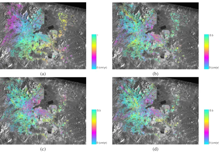
Fig. 9. LP difference maps between PS and SBAS velocity field. (a) at PS step 1, σLP=3.3 mm/yr. (b) at PS step 1, with removal of the residual orbit ramp, σLP=1.2 mm/yr. (c) at PS step 2, with removal of the residual orbit ramp, σLP=1.1 mm/yr. (d) at PS step 3, with removal of the residual orbit ramp, σLP=1.1 mm/yr. A colour cycle represents 1 cm/yr in (a) and 0.5 cm/yr in (b-d).
−0.8 −0.6 −0.4 −0.2 0 0.2 0.4 0.6 0.8 0 2 4 6 Normalized distribution HP, step 1 LP, step 1 (a) −0.8 −0.6 −0.4 −0.2 0 0.2 0.4 0.6 0.8 0 2 4 6 HP, step 2 LP, step 2 (b) −0.8 −0.6 −0.4 −0.2 0 0.2 0.4 0.6 0.8 (PS−SBAS) velocity difference in cm/yr
0 2 4 6 Normalized histogram HP, step 3 LP, step 3 (c) −0.8 −0.6 −0.4 −0.2 0 0.2 0.4 0.6 0.8 (PS−SBAS) velocity difference in cm/yr
0 2 4 6 HP, v < 2cm/yr HP, v > 2cm/yr (d)
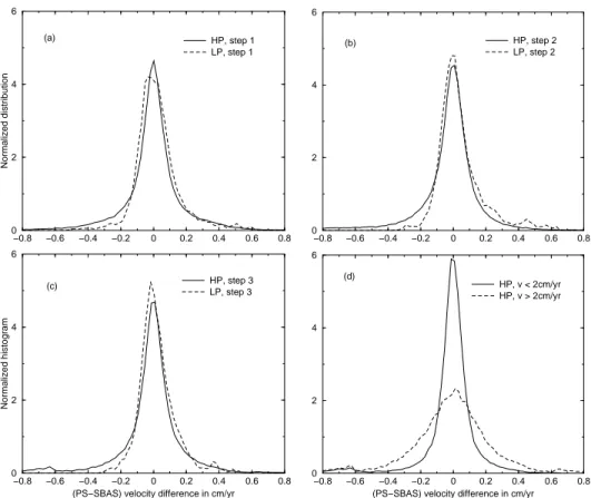
Fig. 10. (a, b, c) : Normalized histograms of PS-SBAS differences of HP (continuous lines) or LP (dashed lines) filtered maps, at PS steps 1, 2, 3 respectively. (d) Normalized histogram at PS step 3 of HP filtered difference map, separating points located outside (with v > 2 cm/yr) or inside (with v < 2 cm/yr) the main subsiding area.
Fig. 11. HP difference map between PS and SBAS velocity field at PS step 3, σH P=1.1 mm/yr. A colour cycle represents 1 cm/yr.
0.5 rad 0.75 rad 1 rad 1.25 rad 1.5 rad 0 rad 6 rad 3 rad 4.5 rad 1.5 rad (a) (b)
Fig. 12. (a) Zoom on the PS phase standard deviation defined during temporal unwrapping at PS step 1. (b) Zoom on nonlinear deformation detected by the SBAS approach. (a) and (b) correspond to the same area. The areas with the highest nonlinear deformation (red to yellow in (b)) correspond to areas with high σ values (in green in (a)).
−7 −6 −5 −5 −5 −4 −4 −3 −2 0.0 0.2 0.4 0.6 0.8 1.0 1.2 1.4
Phase standard deviation (rad)
0 2 4 6 8 10
Amplitude of non linear motion, SBAS (rad)
−6 −4 −2
log (points)
Fig. 13. PS phase standard deviation (σ) as a function of the amplitude of the nonlinear motion (ϕnl) computed by the SBAS approach. Each PS is shown by a dot. The background color map represents the PS density with a log10 scale and is evaluated by Gaussian statistics.
Fig. 14. HP filtered subsidence velocity map obtained using the SBAS approach, surperimposed on the radar amplitude map. The figure is drawn in radar geometry. The black rectangle delimits the area depicted in Figure 12. Note that the color scale saturates towards large positive (excess subsidence) or negative (relative uplift) velocities.
(a) (b)
Fig. 15. Comparison of HP filtered subsidence velocity maps obtained using the SBAS (a) and PS (b) approaches, surperimposed on the radar backscatter amplitude map. The subway station locations are slightly offset towards the West in order not to mask the velocity field. This figure can be compared to Figure 11 in [14].