Combining multiple structural inversions to constrain the solar modelling problem
Texte intégral
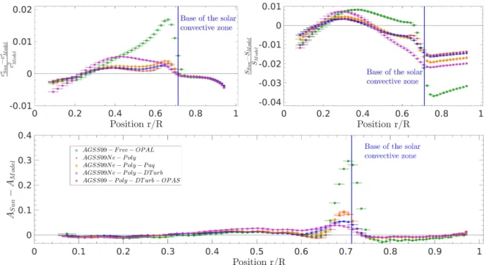
Figure


Documents relatifs
The proposal allows the algorithmic resolution of unknown objects in the directory and in the absence of 1993 X.500 Directory Standard implementations provides an interim
Service type templates define the syntax of service: URLs for a particular service type, as well as the attributes which accompany a service: URL in a service
В данной статье мы рассмотрим проект с открытым исходным кодом – SCAP Workbench [9], как основу функци- онального анализа для
The heuristic evaluates the inversions for placing the right and left elements, and then applies the inversion with least cost.. If a lock inversion does not exist, then the Left
It has been shown that, for some problems of structure and motion estimation, the use of the L ∞ -norm results in a pseudoconvex minimization, which can be performed very
For the initial distribution of the maximum entropy models, we used the model with the best test performance so far, the four-gram deleted interpolation model on the
First, the shortest path, 7r say, may be found by a shortest path algorithm (e.g. Dijkstra's algorithm or, preferably, a label- correcting algorithm [5]) applied to find the
C'est-à-dire que l'image de n'importe quel cercle, par une inversion, sera un cercle, ou une droite (le plus souvent un cercle, mais pas de même rayon!) ; l'image d'une droite sera
