The 1-dimensional [lambda]-self shrinkers in R² and the nodal sets of biharmonic Steklov problems

The 1-dimensional A-self shrinkers in R2 and the

nodal sets of biharmonic Steklov problems

by

Jui-En Chang

Submitted to the Department of Mathematics

in partial fulfillment of the requirements for the degree of

Doctor of Philosophy in Mathematics

at the

MASSACHUSETTS INSTITUTE OF TECHNOLOGY

June 2016

@

Massachusetts Institute of Technology 2016. All rights reserved.

Author ...

Certified by.

Signature redacted

of Mathematics

May 9, 2016

Signature redacted

William P. Minicozzi II

Professor of Mathematics

Thesis Supervisor

Signature redacted

Accepted by...

Alexei Borodin

Chairman, Department Committee on Graduate Thesis

MASSACHUSETTS INSTITUTE OF TECHNOLOGY

JUN 16 2016

LIBRARIES

The 1-dimensional A-self shrinkers in R

_{and the nodal sets of}

biharmonic Steklov problems

by

Jui-En Chang

Submitted to the Department of Mathematics on May 9, 2016, in partial fulfillment of the

requirements for the degree of Doctor of Philosophy in Mathematics

Abstract

This thesis contains two of my projects. Chapter 1 and 2 describe the behavior of 1-dimensional A-self shrinkers, which are also known as A-curves in other literature. Chapter 3 and 4 focus on the estimation of the asymptotic behavior of the nodal set of biharmonic Steklov problems.

Chapter 1 gives the background of mean curvature flow and the importance of self-shrinkers as solitons of the flow equation. We also introduce the background of the A-hypersurface and explain how this is related to the self shrinkers. In chapter 2, we examine the solutions of 1-dimensional A-self shrinkers and show that for certain

A < 0, there are some closed, embedded solutions other than circles. For negative A

near zero, there are embedded solutions with 2-symmetry. For negative A with large absolute value, there are embedded solutions with m-symmetry, where m is greater than 2.

Chapter 3 focuses on the background of spectral geometry. Several eigenvalue problems are introduced. We have a brief survey of some of the important problems such as the asymptotic distribution of the eigenvalues, the shape optimization problem and the bound of nodal sets. This project focuses on establishing a lower bound of the measure of the nodal set. In chapter 4, we use layer potential to establish that the boundary biharmonic Steklov operators are elliptic pseudo-differential operators. Thus we are able to establish lower bounds on both the measure of boundary nodal sets and interior nodal sets for biharmonic Steklov eigenfunctions.

Thesis Supervisor: William P. Minicozzi II Title: Professor of Mathematics

Acknowledgments

First, I thank my advisor William Minicozzi for valuable advice and guidance. He offered me the opportunity to transfer from Johns Hopkins University to MIT, and has generously given me financial support. He also opened my eyes to many interesting topics in differential geometry.

I appreciate the help from Quang Guang, who also transferred from Johns Hop-kins University. In the process of transferring, we faced uncertainty and needed to acclimate to the new environment together. He also gave me much meaningful con-versation about our work and life in general.

At MIT, I am so thankful to have a group of friends in the MIT graduate Christian fellowship. It is so good to have a community here that faces the same difficulties as

I do. Thank you for your companionship, emotional support and prayers.

I want to thank my parents and my brother. Even though my family is in Taiwan,

they always support me. They have patience and love to comfort me when I am nervous and anxious. I want to thank my girlfriend who is always so cheerful and optimistic. She always encourages me not to lose hope. I could not finish this thesis without their encouragement and prayer.

Last and the most important, I want to thank God for. granting me courage and peace to go through all the ups and downs on this journey. There were struggles, but from the grace of God, I grew from them and became more and more mature.

Contents

1 Background of mean curvature flow

1.1 Mean curvature flow ...

1.1.1 Properties of mean curvature flow 1.1.2 Huisken's monotonicity formula . 1.2 Self-shrinkers . . . . 1.2.1 Classification of self-shrinkers . .

1.3 A-hypersurfaces . . . .

1.3.1 Gaussian isoperimetric problem

1.3.2 Classification of A-hypersurfaces 1.4 M y results . . . .

1.4.1 The case for A < 0 . . . . 1.4.2 The case for A > 0 . . . .

2 1-dimensional A-self shrinkers

2.1 Setting up the ODE system . . . . 2.1.1 Periodicity of the solution . . . . 2.1.2 Change of angle in a period . . . . 2.2 The behavior of the solutions . . . .

2.2.1 The behavior of the solution when r is near minV . . 2.2.2 The behavior of the solution when r7 is near infinity

2.2.3 Existence of closed solutions and embedded solutions

2.3 Relation between A and AO . . . .

2.3.1 Alternative proof of theorem 1.4.7 given by Guang. .

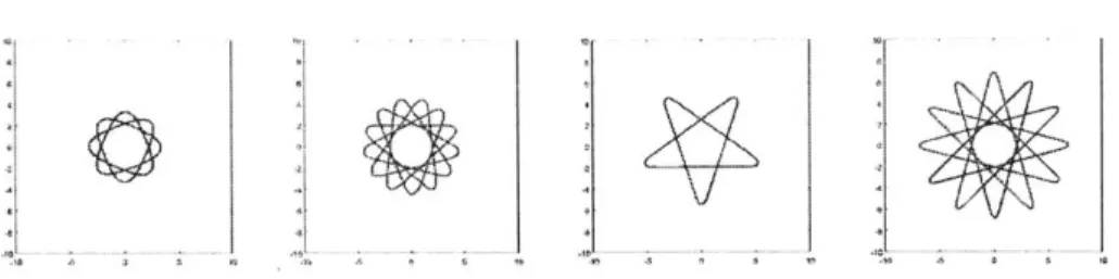
11

2.4 Simulation of the curves . . . . 2.4.1 A > 0 case . . . . 2.4.2 A < 0 case . . . . 3 Background of spectral geometry

3.1 Eigenvalue and eigenfunction of Laplace operator . . . . . 3.1.1 Asymptotic behavior of the eigenfunctions . . . . . 3.1.2 Nodal set and nodal domains . . . . 3.2 General setting of spectral problems . . . . 3.3 Spectral problems on a compact manifold with boundary . 3.3.1 Laplacian spectral problems . . . . 3.3.2 Bilaplacian spectral problems . . . .. 3.4 Spectral problem of boundary Steklov problems . . . .

3.4.1 Harmonic Steklov problem . . . . 3.4.2 Biharmonic Steklov problems . . . . 4 Nodal sets for biharmonic Steklov problems

4.1 Some basic properties for the biharmonic Steklov problem 4.2 Layer potentials . . . .

4.2.1 LP estim ates . . . . 4.3 Lower bound for the vanishing set of AeA . . . . 4.4 Lower bound for the interior nodal set . . . . 4.4.1 Upper bound for !VAe . . . . 4.5 Lower bound for the boundary nodal set . . . .

43 43 44 47 . . . . 47 . . . . 49 . . . . 50 . . . . 54 . . . . 56 . . . . 57 . . . . 60 . . . . 63 . . . . 63 . . . . 65 69 . . . . 70 . . . . 72 . . . . 77 . . . . 80 . . . . 87 . . . . 89 . . . . 92

List of Figures

2-1 Solutions for A = 0.19, A O = ', , ,

5 , respectively. . . 44

2-2 Solutions for A = 0.726, AC = 87r _{5' 2'} 3,r 10,, 4, respectively. _{7 3'} . . . . 44

2-3 Embedded solutions for different A's . . . . 44

2-4 Solutions for A = -2, A = , 13, L, 3, respectively. . . . 45

2-5 Solutions for A = -3, A4r= , , , respectively. . . . . 45

Chapter 1

Background of mean curvature flow

1.1

Mean curvature flow

We start with the variation of a surface in Euclidean space. Let E"

c

hypersurfaces. When the surface changes with respect to t, the area, which is a function of the surface, also changes with respect to t. We can differentiate the area

with respect to time at t = 0 and get the following first variation formula:

df

-- I Area(Et) = f(OtF(x, 0), HN)do-(x),(..)

dt

t=o

where N is the unit normal vector on E and H is the mean curvature of E. Note that if {ej} is a local orthonormal frame of E, the mean curvature H is defined as EZ(VeN, e1), which changes sign if the unit normal vector points in the opposite

direction.

From the first variation formula, in order to have the most rapid descent of the area at any time, the variation vector field OtF should be proportional to -HN. A family of hypersurfaces Et in Rn+1 satisfies the mean curvature flow(MCF) if

where N(t) is the unit normal vector and H(t) is the mean curvature of the hyper-surface Et at x. This is the negative gradient flow of the area functional.

Example 1.1.1. The following are some examples of MCF:

1. If E is a minimal surface in Rn+1, i.e. the mean curvature H = 0. The flow is given by Et = E. The surface does not move at all. This is the most trivial example.

2. The generalized cylinder and the sphere: Et = Sk(V-2kt) x Rn-k in Rn+1 with

1 < k < n and t ranges from -oo to 0. The surface shrinks to {0} x Rn-k at time t = 0 and becomes extinct.

3. The curves Et = (s, - log cos s

+

. We can generalize this example to higher dimension and find rotationally symmetric solution which move by translating along the x.+1 direction in Rn+1.

For the examples given above, the shape of the surface is the same along the flow. Unfortunately, in the general case, the behavior is complicated. Usually, we cannot express the solution explicitly and singulatities may occur due to the nonlinearity of the differential equation.

1.1.1

Properties of mean curvature flow

For the one dimensional curve in R2

, the mean curvature flow is also called the curve shortening flow. Grayson[28 proves the following:

Theorem 1.1.2 (Grayson[28]). Let C(., 0) : S' -+ R2

be a smooth embedded curve in the plane. Then C : S1 x [0, T) exists, satisfying

64C = kN, (1.1.3)

where k is the curvature of C, and N its unit inward normal vector. C(-, t) is smooth for all t, it converges to a point as t -+ T, and its limiting shape as t -+ T is a round

circle, with convergence in the C"O norm.

The result is established by showing that embedded curves will first become convex at some time. According to Gage and Hamilton[261, they then will become round and extinct at a point. This completely characterizes the behavior of the 1-dimensional closed embedded case.

For the higher dimensional case, the behavior of the flow is more complicated. Since the flow equation is a nonlinear heat equation, one of the most important tools for the study of MCF is the parabolic maximum principle. There are some properties which are preserved under the flow. The reader may refer to [21]:

1. If two surfaces are disjoint, they remain disjoint under the flow.

2. If the original surface is embedded, the surface remains embedded.

3. If the original surface is mean convex, i.e. H > 0, the surface remains mean

convex.

4. If the original surface is convex, it remains convex.

For the last case, the behavior of the flow is similar to the one dimensional case. Huisken[341 generalizes the result of Gage and Hamilton[26] to the higher dimension.

Theorem 1.1.3 (Huisken[34J). If E', n > 2, is smooth, convex and compact without

boundary, then the mean curvature flow Et exists on a maximal finite time interval

[0, T) and Et converges to a single point as t -+ T. The surfaces Et converge to a round sphere after appropriate rescaling.

For general non-convex hypersurfaces, even though the surface is embedded, the singularities may occur before the flow becomes extinct. The topology may change when a singularity occurs. Therefore, the study of the singularity is important in

1.1.2

Huisken's monotonicity formula

Huisken's monotonicity formula is a powerful tool to study what happens before the singularity. Define 4 on Rn+1 x (-oo, 0) by

<P(x, t) = (-47rt) ~e! . (1.1.4)

<b is the backward heat kernel defined on R' and extended to R1'+. Huisken proves the following theorem

Theorem 1.1.4 (Huisken[33]). If Et satisfies the mean curvature flow, then we have the formula

4)(x, t) d-t (x) = D - b(x

,t)|IH

|

where do-t(x) is the surface element on Et.

Note that if Et is flowing by MCF, for all constant y > 0, the parabolic scaling

pE -2t is also a solution of MCF. This quantity f <b(x, t)dut(x) is invariant under the parabolic scaling, that is, f, <b(x, t)do-t(x) = f <)(x, pit)do-(x).

The first corollary we can get from this theorem is that the quantity fr 4(x, t)dut(x) is non-increasing in time. As the time goes on, the surface will have less and less f <b(x, t)d-t(x) value. Therefore, the bound of the initial integration gives a restric-tion of the first singularity.

Without loss of generality, we can translate the first singularity to the origin of Rn+1 x R. According to Huisken's monotonicity formula, all the parabolic scaling with p > 1 will give us a mean curvature flow with less fj2 <D(x, t)d-t(x) value and with the first singularity occurring at the origin of the product space. Together with Brakke's weak compactness theorem for MCF, there exists a sequence of pi -+ 00 such that tiZpI2, will converge to a limiting flow E'. This flow is called a tangent

flow at the origin and the integration of the backward heat kernel is constant on the flow. This gives us information about the singularity.

Remark 1.1.5. If we take a different sequence of # -+ o0, the problem whether they will converges to the same tangent flow is still open. This is the uniqueness of the tangent flow problem.

1.2

Self-shrinkers

For a tangent flow at a singularity at the origin, the integration of the backward heat kernel is constant. From Huisken's formula, we can conclude that

HN+-=O (1.2.1)

2t

everywhere. At any time, note that t < 0, the flow Otx = -HN = x _2t is moving by scaling inward with respect to the origin and reparametrization on the surface.

If we consider the flow which moves by scaling with respect to the origin and has a singularity at the origin of the product space, it should be of the form f(t)E. For this type of solution, the space and the time variable in the mean curvature flow equation can be separated and solved independently. Put this into the flow equation, we have

f'(t)x'(to) - - -HN = -H(to)f (t)-'N(to). (1.2.2)

at

Therefore, the scaling function satisfies

f'(t) f(to) f'(to) f(t)

If we want to find solutions with a singularity at t = 0, the solution will be

f

Et = V'-E-1

.

infor-maiton of E-1 to describe the flow. The hypersurface E_1 satisfies

H =X .N) (1.2.5)

2

This equation is called the self-shrinker equation, which express the t -1 surface of a solution which shrinks with respect to the origin and becomes extinct at time t = 0. If we consider the equation satisfied by the tangent flow, we will see the tangent flow at a singularity is a self-shrinker. Therefore, self-shrinkers are models of the singularities.

In the previous examples of mean curvature flow, generalized cylinders and the sphere flow by scaling with respect to the origin. The plane R' which passes through the origin is minimal and thus it is fixed in the mean curvature flow. It is also a cone which is invariant under the scaling with respect to the origin. Therefore, the minimality and invariance under scaling make it satisfies the self-shrinker equation.

1.2.1

Classification of self-shrinkers

For 1-dimensional self-shrinkers in

R

character-ized the closed solutions in the following theorem.

Theorem 1.2.1 ([21). Let y : S' -+ R 2 be a unit speed closed curve representing a

homothetic solution of the curve shortening flow. Then y is an n-covered circle Y,, or -y is a member of the family of transcendental curves {1,n} having the following description: if n and m are positive integers satisfying 1 < n < ", there is (up to

congruence) a unique unit speed curve -yn, : S' -+ R2 having rotation index n and closing up in m periods of its curvature function k > 0, a solution to the equations

B" + 2w2_{(eB - 1)}

₌

2109k (1.2.6)

for some constant w.

If (r, 0) are polar coordinates with origin at the center of mass of then k and r are related by k - Ce-wi' for some constant C.

Since the rotation index n is always greater than 1, the curves Ynm are not em-bedded. As a result, circles are the only closed, embedded solutions.

It is worth mentioning that Halldorssen[30 classifies all the curves which move by scaling(shrinking or expanding), rotation or a combination of scaling and rotation. The same author[31] also classifies the self-similar solution for the curve shortening flow in the Minkowski plane R1,1.

For higher dimensional cases, in R1, Angenent[3] discovered a well-known solution, "the Angenent's doughnuts", which is an embedded rotationally symmetric solution with the topology of a torus. This example can be generalized to any higher dimen-sions as an embedding of S" x S1 into Rn+1 with rotational symmetry in the first n coordinate. Moller[44] constructs more closed embedded solutions. For noncompact examples, the reader can refer to Kleen and Msller[36. These examples have different topology and make the complete classification of self-shrinkers almost impossible.

In what follows, we list some of the most important literature concerning the classification of the self-shrinkers. First, Huisken[341 classifies the self-shrinkers under the condition of nonnegative mean curvature, bounded second fundamental form and polynomial volume growth.

Theorem 1.2.2 (Huisken[34J). If E is a smooth self shrinker in R'+1, with nonneg-ative mean curvature H > 0, then E is one of the following:

1. Sn,

2. Sn-' x R'"

3.

R

where y is one of the homothetically shrinking curves in R2

found by Abresch and Langer in Theorem 1.2.1.

We include the proof of the compact case here. This illustrates the most basic idea in the classification. First, we introduce the drift Laplacian L, which is defined as

,Cf

X 1

This operator is self-adjoint in the Gaussian weighted space. For functions u, v which are controlled at infinity such that we can do the integration by parts, we have

Ju(v)e- = - j(Vu, Vv)e-4do = (Lu)ve-4do, (1.2.8)

The following proof is adapted from [341, [331.

Proof. On the compact surface E, let el, e2, -- , e,, be an orthonormal frame on E. Let A = (hij) be the second fundamental form. We can differentiate the equation (1.2.5) and get the following

1

LH=

_,

21 (1.2.9)

hijViVjH =

IA|2

2 2

From Simon's identity, we have

LIA12 = -21A 4 + JA12 _{+ 21VA1}2_{. (1.2.10)}

Since H > 0 we can compute the drift Laplacian of .

H2 _A

H

H2

Move all the terms with to the same side, multiply the equation by H2

e- 4 and

integrate. We have

2V |2H2e-

d=

[C(A

H2e-+d-H

H

= Jdiv[H2 e-V(-)]d- = 0.

Therefore, we can conclude V-A 0, the tensor Ais parallel. We have IhjjViH

-VjhjjH12

= 0. From the Codazzi equation and the curvature tensor vanishes

iden-tically in R+ 1, IhjjVjH - hjjVjH12

that el is parallel to VH. In this case, VjH = 0 for all j > 1. Therefore,

n

0 = hi3V1H - haV3H12 =

21VH

(1A1

We have either

IVH

h 2g.. For the case that

IVH

curvature is constant and therefore it can only be a sphere in the compact case. If A12 = En h~i, it is only possible when hi = 0 except (i, j) = (1, 1). We can deduce that JA12

= H2. Integrating equation (1.2.9) on E, we have

H 3do- = -- H + (xT V

H)do-1

do- (1.2.14)

1JHdo - n

+

do.

Therefore, we have - fE Hd- = 0, which is impossible for compact E when n > 1 and H > 0.

For the noncompact case, there are more technical details involved to do the integration by parts. In that case, it is possible for the mean curvature H not to be a constant. This corresponds to the case 3 in the classification. In Huisken's proof for noncompact manifold, some bounds of the growth rate of the second fundamental form and the volume are assumed. Later, Colding and Minicozzi[21 remove the requirement of the second fundamental form bound for the classification result. They also show that the generalized cylinders are generic solutions in the sense that one can perturb a flow to make all the singularities of this type.

If a self-shrinker is also an entire graph over Rn, Ecker and Huisken prove the following:

Proposition 1.2.3 (Ecker and Huisken[24J). If E is an entire graph of at most

poly-nomial growth satisfying the self-shrinker equation (1.2.5), then E is a plane.

For the genus 0 surfaces in R', Simon Brendle establishes the following theorem for the compact case.

Theorem 1.2.4 (Brendle[8J). Let E be a compact embedded self-shrinker in R' of genus 0. Then E is a round sphere.

And the following for the non-compact case

Theorem 1.2.5 (Brendle[8]). Suppose that E is a properly embedded self-shrinker in R' with the property that any two loops in E have vanishing intersection number mod 2. Then E is a round sphere or a cylinder or a plane.

1.3

A-hypersurfaces

Now, we consider the A-hypersurface equation. Let En c Rn+' be a hypersurface satisfying

H = (X +A, (1.3.1)

2

where N is the normal vector on the surface, H is the mean curvature and A is a constant. Our goal is to describe the behavior of the 1-dimension solutions in R2

1.3.1

Gaussian isoperimetric problem

The equation (1.3.1) is first studied by McGonagle and Ross[431 and is named as A-hypersurface in the work of Cheng and Wei[17. The equation arises in the Gaussian isoperimetric problem: In Rn+1, the weighted Gaussian volume element is given by dV, = exp(- 1x1 )dV, where dV is the volume element induced by the Euclidean metric. For the case that E is closed and E = 9Q for some bounded region Q C R+ 1, let the r-neighborhood of Q, Q, {x E R n+1Idist(x, Q) < r}. The boundary measure is defined by

Vti(Qr) -Vji(Q)

PM lim inf .(1.3.2)

r-+O

r

This measures the relative rate of change of Gaussian volume for small change from Q to Qr. When E is smooth, the boundary measure P,(Q) = A4,(E) = f, don, where

do-is the weighted Gaussian area element defined by do, = exp(- k!if)du. The Gaussian isoperimetric problem asks: Among all regions with the same weighted volume Vo, which one has the least weighted boundary area? The answer to this problem is given by Borel[71, Sudakov and Tsirel'son[51: The half space minimizes the weighted boundary area.

The problem above can be considered locally as follows. Let F : E x (-E, c) -+ Rn+1 be a smooth, normal variation which fixed the weighted volume, OtF(x, 0) = uN when t = 0. We have

dV(Q)|t=o = ue do-,

H (, N)

~(1.3.3)

d (x N

-P(E)-t=O =U(H -

2

dt 2

Let E be a surface minimizing the weighted boundary area among all surfaces enclos-ing the same weighted volume. Because of the minimality, the surface is a critical point for all variations that fix the enclosed weighted volume. We can deduce the equation (1.3.1). This equation is defined on E locally and it can be studied even if E does not enclose a region. The solutions can be thought of as the critical points to the weighted area functional. In McGonagle and Ross' work[431 they show the hyperplane is the only stable smooth solution to the Gaussian isoperimetric problem in terms of the second derivative of the weighted Gaussian area functional.

Remark 1.3.1. In the special case A = 0, the equation becomes the original shrinker equation (1.2.5). This comes from the fact that the self-shrinkers are also the crit-ical points of the weighted area functional under any variation, not only the volume preserving ones, in Gaussian space. Therefore, we call equation (1.3.1) the A-self

shrinker equation in my work.

Remark 1.3.2. A-hypersurface also arises in other studies. For example, it plays an important role in the study of weighted volume-preserving mean curvature flow by Cheng and Wei[17].

1. The hyperplane Rn which is A away from the origin in the normal direction.

2. The cylinder Sk( A2 + 2k - A) x Rn-k

3. The sphere Rn(vV 2

_+2n

- A).

The examples above admit properties such as polynomial volume growth and con-stant mean curvature. They also admit good symmetry. It is important to investigate under which assumption we can deduce that a A-hypersurface is one of the above.

Some rigidity results can be found in [161, [18], [291 and

143].

1.3.2

Classification of A-hypersurfaces

The problem of classification of A-hypersurfaces can be regarded as a generalization of the case of self-shrinkers. The H > 0 case in self-shrinkers is now replaced by H - A > 0 and discussed in the work of Cheng and Wei[171. However, this is not enough to guarantee the round solution. Further quantities arise in the differentiation, and we also need the condition about the following quantities:

1A1

(1.3.4) trA3

₌

>hihkhki,

i,j,k

where hij is the second fundamental form corresponding to an orthonormal frame. Now, the result of the classification is

Theorem 1.3.4 (Cheng, Wei[17J). Let E be an n-dimensional embedded A-hypersurface in Rn+1, either compact or complete with polynomial area growth. If H - A > 0 and A(2trA 3(H -A) - Al2) > 0, then E is one of the standard round solutions in example

1.3.3.

Laplacian of the curvature terms are given by 1

LH= -H +A 1A - H), 2

L1A1

_1A1

_21A1

_21VA1

, (1.3.5)

1 6 V(H - A)12 _21A12_{(H - A) - H}

- 6 +.

(H

-

_-

_-

The proof is established by replacing 1 in the proof of the self-shrinker case by

A2 . There will be an extra term involving A(2trA3(H - A) -

IA!

),

Remark 1.3.5. We cannot remove the condition A(2trA3

(H - A) - Al2

) > 0. My work, which will be introduced in the next section, shows that when A < 0 there are 1-dimensional solutions in R 2 which are not the standard circle.

1.4

My results

My work focuses on the behavior of the equation (1.3.1) in R2. In what follows, to simplify the equation, we scale the curve by a factor of v/2 to make the constant 1 become 1 and use the 1-dimensional curvature k in place of mean curvature H. The equation becomes

k

=

Generally, the behavior of the solution is described by the following theorem. We state the theorem in a way similar to the theorem given by Abresch and Langer so that the reader can make a comparison.

Theorem 1.4.1. The curvature function k > 0 of the A-curves satisfies

B" = 2(1 + Ae2 - eB), B = 2logk. (1.4.2)

1r2

Also, let r be the distance to the origin. Then k and r are related by k = Ce2 for some constant C.

If n and m are positive integers satisfying

1v'

A

n

1V'

A

min{ + 1} < - < max{ + 1}, (1.4.3)

2' 2 A2₊₄

+ M 2' 2 A2 ₊₄

then there is a closed curve -yn, : S' -+ R2 having rotation index n and closing up in m periods of its curvature function k > 0, which is a solution to the equation (1.4.1). Remark 1.4.2. In the theorem above, we give a sufficient condition of existence of solutions. The condition may not be a necessary condition. Therefore, in each of the following results, further work is needed.

Remark 1.4.3. For the case k < 0, we can choose the normal vector N to be the opposite. In that case, it would correspond to a solution with the curvature replaced with -k and the A replaced with -A. More details will be given in section 2.1.

1.4.1

The case for A <

0

From this theorem, for A < -, there are solutions with n = 1 and therefore embed-ded.

Theorem 1.4.4. For A < 7, there exists an embedded solution. The embedded solution admit m-symmetry for some m > 2.

Remark 1.4.5. From the behavior of the differential equation, we are able to extend the range for A. Actually, there exist 6 > 0 such that there is such embedded solution for A < 7 + .

For the embedded solution with 2-symmetry, it is subtle because 'is either the lower bound or the upper bound of ", so the theorem 1.4.1 cannot guarantee the existence of an embedded solution with change of angle exactly 7r in a period. Further detail for the behavior of the differential equation when energy is near infinity is needed to establish the existence of solution with 2-symmetry.

Therefore, for certain negative A, there exists embedded solutions other than the circle.

Unlike the result of Abresch and Langer[2 that for the A = 0 case, the circle is

the only closed embedded solution, we surprisingly find other embedded solutions. This affects the understanding of the rigidity problem about the classification of A-hypersurfaces. If we product the curve with R"4, we obtain a A-hypersurface in Rn+1

which is topologically S' x R 7 with non-vanishing mean curvature and polynomial area growth. However, this is not the standard round cylinder as in example 1.3.3. This is the A-hypersurface analogue of the case 3 in theorem 1.2.2.

We can also compare the result with the isoperimetric problem in Euclidean space, where the critical surface to the area functional should admit constant mean curva-ture. Thus the only 1-dimensional solutions of the isoperimetric problem in R2 are circles. However, the embedded solutions, which are the critical surface in the Gaus-sian isoperimetric problem, can be other than circles.

1.4.2

The case for A >

0

For positive A, the behavior is similar to the self-shrinking curves. Since the theorem 1.4.1 gives only a sufficient condition, we need to compare the change of angle with the self-shrinkers and use Abresch and Langer's result to rule out the possibility of embedded solutions.

Theorem 1.4.7. When A > 0, there are no embedded solutions to the equation (1.4.1)

with k > 0.

Remark 1.4.8. It is worth mentioning that Guang[29] establishes the same result as

in theorem 1.4.7 with a different proof. He considers the part of the curve where the curvature decreases from the maximum to the minimum.

Chapter 2

1-dimensional A-self shrinkers

In this chapter, we are going to establish the result of 1-dimensional A-self shrinkers. This chapter will be structured as follows:

In section 1, starting from the defining equation, we derive an ODE system for the 1-dimensional A-self shrinkers. The approach used here is similar to that in the work of Halldorsson[301. This is a powerful tool to study the curves in R2, which describe the curve by its tangent component and normal component.

In section 2, we define the energy qj for a solution and analyze the behavior of the solution for the extreme cases: The energy is near the minimum and the energy is near infinity. We first get the change of angle at the both extreme case and use continuity to establish the theorem 1.4.1. As mentioned before, we need more detail when the energy is near the minimum and near infinity to establish theorem 1.4.6 and 1.4.4.

In section 3, we fix the relative energy and find the relation between AO and A.

We can compare the change of angle with the case of self-shrinker in the work of Abresch and Langer[2] and establish theorem 1.4.7.

In section 4, we use Matlab to get numerical solutions which approximately solve the equation. Some pictures of the curves are provided for better understandings of the behavior for each of the different cases in the main theorems. We also give some conjectures about the behavior of the solution here.

2.1

Setting up the ODE system

For a curve x(s) E R2 _{parametrized by arc length s, we have}

d

-X = T7

ds _ds (2.1.1)

-T= kN, ds

where T and N are the tangent vector and the normal vector of the curve, respectively. Note that for any curve in R2_{, we have two possible choices of N: either rotate T}

clockwise by E or -. If we let N- = -N, k = -k, we have kN =k~N. Therefore, we have

k~ = -k = (x, N) - A = -(x, N-) - A. (2.1.2)

This tells us that selecting the opposite normal vector will change the sign of k and result in a solution corresponding to -A.

Using the method as in Halldorsson's work[30], we decompose the position vector x into the tangent part and the normal part. The curve can be reconstructed by these data up to a rotation. Let T = (x, T), v = (x, N). We can obtain the ODE system

{

sdv -kT - AT.(2.1.3)

The equilibrium is the point where r = v = 0. They are given by (0, vz), where

0 A v/A 2 +4

A A 4(2.1.4)

2

are the positive and the negative solutions of the equation v2 - Av -1 = 0, respectively. At the equilibrium, the curvature is a nonzero constant. It corresponds to the circle centered at the origin. For (0, i ), it is a circle of radius vj with the normal pointed outward and k < 0. For (0, V'), it is a circle of radius -v = jv | with the normal pointed inward and k > 0. Also, note that (T, v) = (s, A) is a solution which

corresponds to a line with the minimum distance to the origin equal to A. From now on, without loss of generality, we only consider solutions with k > 0. They are the solutions with the trajectory contained in the half plane {v < A} of T - v space. -For the solutions with k < 0, choose the opposite normal vector and study them as the solutions corresponding to -A with positive k.

2.1.1

Periodicity of the solution

For a solution to the system, the function

F(, v)= (A - v) exp( 2 (2.1.5)

is positive in the {v < A} half plane. Differentiating it with respect to s, we have

d d d d V 2 +T2

F = - (A-v)(V d +d ))exp( 2 )

ds Tk dsd ds2

V2 + 2

(v - A)+ (v - A)(v(v -A)r+ T(1- _{v(v - A)))) exp(- 2}

-0.

(2.1.6)

The trajectory of each solution lies in a level set of F. Since each level set of F is a simple closed curve except the level set {F = 0}, which corresponds to the line mentioned before, we have a uniform lower bound of the speed of (T(s), V(s)) curve away from 0 on each level set. Therefore, the solution (r(s), v(s)) should be periodic in s.

Remark 2.1.1. Note that if x(s) is periodic, then T, v are periodic. But the converse may not be true. Starting from a periodic solution of (T(s), v(s)), the resulting x(s) is periodic only when the change of angle in a period can be expressed as 2, where n, m are positive integers. In this case, the period of x(s) is m times the period of

2.1.2

Change of angle in a period

Now, since k is more directly related to the geometric behavior than v, we use (r, k) as the variable instead of (r, v). Plugging v = A - k into the previous ODE system, it becomes

{ r - I + Ak -k2

and {v < A} becomes {k > 0} in r - k plane. Note that after the change of variable,

we still have the equilibrium at (0, k'), where k' = vj because they satisfy exactly the same equation. However, (0, k') correspond to (0, v ), respectively. The v = A

line in T - V space now becomes k = 0 line in r - k space. Also, the function F

becomes

F = ke 2 (2.1.8)

From now on, we will work in the {k > 0} half space. For simplicity, write k = k+

and we will not use k' anymore. Let B = 2 log k. We have 4 = 2- and

d

d 2 = _{2- =-2+2k(A-k)=2+2Ae -2e (2.1.9)}

ds

Remark 2.1.2. This equation can also be derived from the A-hypersurface analogue

of equation (1.2.9). If we apply the Laplacian to the scaled equation

H = (x,N) - A, (2.1.10)

the result would be

AH

HIA1

_.

In 1-dimensional case, together with the knowledge of xT = TT we can get the same second order equation. We derive the equation from the 1-dimensional frame T, v to

Multiplying both sides by L and integrating with respect to s, we get

( dB + 2eB - 4Ae" - 2B = -4logF - 2A2. (2.1.12) If we define FA = F -exp A2, V(B) = eB 2Ae - B, the equation becomes

--(--)2+ 2V(B) = -4 log F\. _(2.1.13)

2 d s

B B

The minimum of V(B) is attained when d'(B) = 0. e - Ae -1= 0. e k. This corresponds to the equilibrium at (0, k) and min V(B) = -Ak - 2 log k' + 1. Now, since the value (4AB) 2 is always nonnegative, the maximum value V(B) can attain is

-2 log F.

Now, define the energy q7 of the curve by 'q = -2 log FA. The range of the energy is from min V(B) to infinity. For any r in this range, we can find the solutions B,- < B7

of V(B) = rq. Considering the differential equation of B, we get 1( )2 _{+ 2V(B) = 27,}

2 ds _(2.1.14)

dB_

d = k2V2-V(B). ds

Therefore, the length of the curve in a period is given by ,B dB _"

ds = 2 j (d ) dB =( dB, (2.1.15)

B ds B 1 (B)

and the change of the angle in a period is given by

B B

AO=

J JB; Vq - V(B)

In order to simplify the calculation, we can switch the variable back to k. Let k

-B 2

of angle in a period of curvature, AO, is given by

A =. (2.1.17)

2.2

The behavior of the solutions

Now, we will focus on the behavior of AO when the energy q varies from min V to oo.

2.2.1

The behavior of the solution when

r

is near minV

The following focuses on the behavior of AO. When the energy is near the minimum, the behavior is closed to a simple harmonic oscillator.

Lemma 2.2.1. For any potential function V C C2, at a local minimum k' with

positive second derivative, let k7 be the largest solution of V(k) = 77 which is below

k' and let k+ be the smallest solution of V(k) =,q which is above ko. We have

lim

A

Jk / -V(k) V"(k)

where ' denotes d

Proof. First, note that for the case in which the potential is quadratic, V(k) = V(k )+

V"(k)( kk*)2

a simple calculation shows that

Sk+

dk

k -V(k) V"(k1)

for any q > V(k0) and is independent of r.

For arbitrary potential function V E C2 and E > 0, there is 6 > 0 such that for all V(k0) < q < V(k0) + 6, we have IV"(k) - V"(k0

)j

[k+, kj].

T-E-We have V_ < V < V+ in (k-, u+,). Therefore, +i dk

J7

dk

-V+(k)

dk

Letting E goes to 0 yields the desired result. L

Proposition 2.2.2. When q -+ min V+, AO approaches 7r-

2

+

Proof. Let q -+ min V+. The derivatives of V(k) with respect to k at the minimum point are

V(2) (k) = 2 + 2(k -2 V(3) (k ) = -4(k) )-3, V(4)(k = 12(ko -4.

Therefore, from the lemma above and recall that k = A+ , we have

(2.2.4) lim AO ij-+min V+ li k17

2dk

=lim/

A

From the result of Chicone[191, since

5(V(3))2 -

4V(2)(

80(ko)-

96((ko)~

_{+ (ko)-}

)

= -16(ko)-

_96(ko)-

_0,

the function AG is decreasing near min V with respect to q7.

(2.2.6)

F-1

Remark 2.2.3. For the case of self shrinkers, we have A = 0. The proposition above gives AG -+ vti2r, as the result in Abresch and Langer[2]. This function is strictly

2

V"l(k) + e

(2.2.3)

increasing with respect to A. When A approaches oc, AO approaches 27r. When A approaches -oo, AO approaches 0.

2.2.2

The behavior of the solution when

r,

is near infinity

Now, we turn our attention to the behavior of AO when the energy approaches infinity. An upperbound of AO is given by the following proposition.

Proposition 2.2.4. For any L > 1,

L 1 1

_O r+2 A-1+ '-+ o(-) (2.2.7)

VL - 1) V/ij- \/ as q goes to infinity.

Proof. In order to get an upper bound of AO, separate the integration into two terms.

(kl? k 77ggk

AO

2dk

J

Ik

i

When 1 < k < k, we want to construct a quadratic function which is larger than V(k) in this interval such that the integration can be computed explicitly. Let

I.+

Ij

- 2Ak is quadratic and passes (1, 1 - 2A), we want to modify this function so that it passes (k4, y). Using scaling, let V(k) = ( (k - 1) + 1)2 - 2A(K 1 (k - 1) + 1). At k = k+, V(k) = V(k) =. At k = 1, V(k) = V(k) = 1 - 2A. The second derivative of V(k) - V(k) is

(V(k) - V(k)) 2(k+ _ 1) 2

- (2 + 2k) <0. (2.2.9)

We can conclude

for any 1 < k < k+. Therefore, we have l 1 k j + 2dk) j1 k+ 2dkg V V~) J, r- V-(k) k - 1 f4 k+ - 1 1 2dv 7) - V2 +

2Av

Ik+

We need an upper bound for Starting from k~+

77 1 '7

A + V/A

2_{+ TV(kn)}

₌

7 - 2 log kc, V(k) = 7 and V'(k) > 2k+j - 2A - 2 for k+ < k < k+, we have

- 2log kc+

k7- k -n

2+-

for 77 large enough. Hence,

log k+ k1+ _ A .- _

C log 7) 2

k+l _ 1 k+ - k+

-

=1+

1O(i

k+ -1 k - 1 Therfore, k 1 2dk V'7 7

-V(k)-k+

₎

+A

+

Now, we are going to estimate the other term. For all L > 1, let k = exp(-- + + JAI). Note that when y is large enough, kL d

L

Ih

2dk

k~7-V(k)

) V(k)+0~ V M)

V

For the first term, since

V(k-)

7,V(k-)

~,V"

L L- 1 k-~ L L k-(2.2.15) (2.2.16) (2.2.11) 1

= O(q- log ?I) (2.2.12)

(2.2.13)

1

+ 0(- -.

for k- < k < k.-4 and 2dk fk L -V (k)< Jk

< 2dv

L

4

j

The second term can be bounded by the following,

Ik

2dk

17

-

(k)

Sl

-Combine the estimation of both terms, we have

AO < r

+

A

+L

L 1

_/

After establishing an upper bound of AO, a lower bound is given by the following:

Proposition 2.2.5. We have A -k- A -k'-A ;> 7r

+

+

)

I

2dk<

vlij

Proof. To get a lower bound of AO, use log k < log k+ when k,, < k < k+. Ik+

AO-

2dk

2dk

k ( + 2logk + A2) _ (k _ A)2

= 7r

+

A-77+ _{2log k,+ A}2

A+ - A =ir + 2sin1

k

Note that in this proposition, we do not require the energy to go to infinity. From this lower bound, we can get a partial proof for the theorem 1.4.7 for the case A > .

Proof. Separate into 2 cases: k,-, < and k-> 1

For the case k, < , applying proposition 2.2.5 yields the result AO > r. For the case k- > , we have V"(u) > 8 in the interval (k-, k,). Let V be the quadratic curve passing through (kg, 7) and (kg, 77) with second derivative equals 8. From the maximum principle, we have V > V in (k'-, k,). Therefore,

AG fkn 2dk

- V (k)

(2.2.23)

77

2dk

2

L2

=~k

r.

Combining both the upper bound and the lower bound, we can get the limit of AG when the energy 7 goes to infinity.

Proposition 2.2.6. For any A, when the energy q goes to infinity,

lim AG = 7r.

?7-+0O (2.2.24)

Proof. As rq goes to infinity, k+ goes to infinity and k,- goes to zero. Therefore, the upper bound and the lower bound established above both approach 7r as 71 goes to

infinity. 11

2.2.3

Existence of closed solutions and embedded solutions

The proof of the theorem 1.4.1 is given by this proposition together with the behavior when 77 is near 0.

Proof of Theorem 1.4.4. For any A < 7, when r, -+ min V+, the limit of AO is less

than 2. When rq is large enough, AO approaches 7r. From continuity, there exist q7 such that AO is exactly Z for some integer m > 2.

A0 is decreasing when rq is near min V. When A = , min, AG0 < g. From the continuity, the range for A can be extend a little higher than -. F

2VW El

Furthermore, from the upper bound, we can get more information for the case A < 0 and r7 large.

Corollary 2.2.7. When A < 0, AO < r for r7 large enough. Proof. Since

L ch< 7+2 A- 1+ g+ s( 1

~-L

- _{I ,F5} ,y for arbitrary L > 1, choose L large enough so that A - 1

+

(2.2.25)

With the knowledge of the behavior of AG for small energy and large energy, we can proof the theorem concerning the case A < 0.

Proof of theorem 1.4.6. For ' < A,

lim

AO

For A < 0, A <r when q is large enough. From continuity, there exists q such that

AO is exactly 7r. l

2.3

Relation between A and

AO

For the case A > 0, the behavior is similar to the original case for self shrinking curve in Abresch and Langer's paper. We want to compare the change of angle with the case A = 0.

Recall k is a function of A. Translate the minimum point of V\(k) to the origin, define V\(u) = Vx(u+ k0) - min 1V, where min V = VA(k) = (k) 2 - 2Ak - 2 log k0. Let ' =7 - min V be the energy relative to the minimum. We have the following theorem:

Theorem 2.3.1. With the setting above, for a fixed O, is increasing with respect to A.

Proof. Note that in this setting,

AO=J 2du , (2.3.1)

where u are the positive and negative solution of f7 = V,(u), respectively.

Now, for a fixed iy, we want to know the relation between A and u when VA = A(u). Differentiate the equation with respect to A, we have

0=2((u+ko)-A (kI) + () 2(u+k)-2(k -A- ) + 2k S _ +k -1 dudk0T2 =2( )2 -Au+k)-1(--u+ )-'2u u+ko dA d U2 + 2k'u - Au du dk' = 2-_ (- +7- )-2u u+k dO dA ru+2k0-A du dk 1 u2+k3 d2 d (2.3.2)

Therefore, du dk' u + kO -- + .(23.3) dA dA u+2ko - A (2.

Since k

we have

dkV

1+

+ k'

(2.3.5)

Since k - A, 2k0 - A, u + ko are all positive, L has the same sign as u, i.e. > 0, 2 < 0.

Starting from /(u) = 2(u + k' - A - ),for any i < i, we want to know the change of the slope of V( at u with respect to A. Differentiating the equation with

respect to A, we have

- (^ (u))

2 (1 +

)(-- +

) -

)

dA

(u + k

dA

dA

(u + ko

u + 2ko - A

(u + ko)(u+ 2k - A)

Note that A - ko < 0 and therefore d (VA((u)) and u have the opposite sign.

Now, fix i, A, < A2. Since L and u has the same sign, we have U- < u < 0 < u+ _qIA < u. Consider the function V, (u) and

+

1 fIA2V\(U+rj,A 2 the

-them have the same value i at u = u . Now, for all fixed i

c

&ZL< = 09 A2 (2.3.7)

Therefore, for any i E (0, i), UtA > UA - (f/ - t), i.e. the graph of (aq7, 6)

lies on the right of the graph of (u

).

V((u+A)

0, it

implies that V\ (u) <

PA\,(u

uE (U 0). Therefore,

AO(#7, A,)

< 2du t7A'X 1

V

(

~

~i),A

VW - x2(u) "l,2 fl,"A1 #7 - A₂(u)

2du =

AO(#,

(2.3.8)

Now, compare the case A > 0 with the self shrinker case.

Proof of theorem 1.4.7. Use the result in Abresch and Langer[2 that when A = 0, AO(, 0) is a decreasing function of 4, lim.qo AO(r, 0) = V2-7r, limq, AO(r, 0) = ir. Hence for all

#7,

AO(,

2.3.1

Alternative proof of theorem 1.4.7 given by Guang

Here, we also include the proof given by Guang for a better understanding.

Alternative proof of theorem 1.4.7 in [29]. Define 0 = arg N, this 0 describe the polar angle of the normal vector and the change of angle in a period is AO as introduced

2du 7-

i ,Ju