HAL Id: hal-01931475
https://hal.archives-ouvertes.fr/hal-01931475
Submitted on 16 May 2020
HAL is a multi-disciplinary open access
archive for the deposit and dissemination of
sci-entific research documents, whether they are
pub-lished or not. The documents may come from
teaching and research institutions in France or
abroad, or from public or private research centers.
L’archive ouverte pluridisciplinaire HAL, est
destinée au dépôt et à la diffusion de documents
scientifiques de niveau recherche, publiés ou non,
émanant des établissements d’enseignement et de
recherche français ou étrangers, des laboratoires
publics ou privés.
To cite this version:
Lynda Khiali, Mamoudou Ndiath, Samuel Alleaume, Dino Ienco, Kenji Ose, et al.. Detection of
spatio-temporal evolutions on multi-annual satellite image time series: A clustering based approach.
International Journal of Applied Earth Observation and Geoinformation, Elsevier, 2019, 74,
pp.103-119. �10.1016/j.jag.2018.07.014�. �hal-01931475�
Detection of Spatio-Temporal Evolutions on Multi-annual Satellite Image
Time Series: A Clustering Based Approach
Lynda Khialia, Mamoudou Ndiatha, Samuel Alleaumea, Dino Iencoa,b, Kenji Osea, Maguelonne Teisseirea
aTETIS, APT, CIRAD, CNRS, IRSTEA, UNIV.Montpellier, Montpellier, France bLIRMM, Montpellier, France
Abstract
The expansion of satellite technologies makes remote sensing data abundantly available. While the access to such data is no longer an issue, the analysis of this kind of data is still challenging and time consuming. In this paper, we present an object-oriented methodology designed to handle multi-annual Satellite Image Time Series (SITS). This method has the objective to automatically analyse a SITS to depict and characterize the dynamic of the areas (the way that the land cover of the areas evolve over time). First, it identifies the spatio-temporal entities (reference objects) to be tracked. Second, the evolution of such entities is described by means of a graph structure and finally it groups together spatio-temporal entities that evolve similarly. The analysis were performed on three study areas to highlight inter (among the study areas) and intra (inside a study area) similarity by following the evolution of the underlying phenomena. The analysis demonstrate the benefits of our methodology. Moreover, we also stress how an expert can exploit the extracted knowledge to pinpoint relevant landscape evolutions in the multi-annual time series and how to make connections among different study areas.
Keywords: Satellite image time series; Object-oriented image analysis; Clustering; Graph Analysis;
Inter-site analysis
1. Introduction
Nowadays, remotely sensed satellite images constitute a rich source of information that can be leveraged to support several applications including food risk prevention, land use planning and mapping, natural habi-tat monitoring, land cover classification and many other several tasks [1]. Advances in satellite technologies and the high images acquisition frequency result into huge amount of remote sensing data that need
effec-5
tive and efficient analytics approaches. Standard tools including photo interpretation and fully supervised approaches are not suitable for dealing with this large amount of spatio-temporal data [2]. In this context, data mining techniques have already shown their usefulness [3] and they seem adequate to extract valuable knowledge to support remote sensing analysis on both single image or Satellite Image Time Series (SITS) data [4, 5, 6].
10
Several data mining approaches are commonly employed to analyse SITS data: supervised [7], unsuper-vised [8, 9] and semi-superunsuper-vised methods [10, 11]. Due to the lack of reference data, unsuperunsuper-vised methods such as clustering are widely employed to explore and mine patterns from remote sensing data. Data clus-tering is the process of partitioning the data into groups where, similar examples are assigned to the same group and non similar examples are assigned to different ones [12].
15
Email addresses: lynda.khiali@irstea.fr (Lynda Khiali), ndiathmamoudou@yahoo.fr (Mamoudou Ndiath),
samuel.alleaume@irstea.fr (Samuel Alleaume), dino.ienco@irstea.fr (Dino Ienco), kenji.ose@irstea.fr (Kenji Ose), maguelonne.teisseire@irstea.fr (Maguelonne Teisseire)
In this work, we propose an unsupervised method to analyse SITS data at object level in order to highlight intra and inter similarity among the different study areas. Two important factors influence the clustering of remote sensing time series: i) the distance measure choice and ii) how data are represented.
Considering distance/similarity measures commonly involved in SITS analysis, the standard choice is the euclidean distance (or one of its variants) [13] due the fact that it is intuitive, easy to implement and
20
parameter free. Conversely, how to represent SITS data in order to exploit as much as possible the available spatio-temporal information remains a challenge and researchers have devoted time and effort to deal with this point [14, 15].
In unsupervised as well as in the supervised analysis, SITS data are mainly exploited at pixel level. For each pixel, a time series is built. The radiometric values of the pixel, in the considered satellite images, are
25
gathered and ordered based on the temporal dimension. Thus, the number of time series is equal to the number of pixels covered by the considered area [14]. The method proposed in [6] analyzes SITS information at pixel level to detect land cover classes. To perform clustering, they compute a distance matrix between pixel time series using the euclidean distance. Then, they run the Affinity Propagation (AP) algorithm [16] on the matrix. The method was evaluated on three data sets, the AP results were compared to those obtained
30
using the K-means and the Agglomerative Hierarchical clustering algorithms. The authors introduce in [17] a method to analyse multi-annual satellite image time series to monitor vegetation areas using the vegetation index. The method analyses the SITS at pixel level, it builds an annual profile which characterizes the pixel evolution on each year. Then, it gathers these representative annual profiles to construct a final sequence to characterize the evolution of a pixel over several years. Finally, a clustering algorithm based on the euclidean
35
distance is employed to characterize the vegetation dynamic.
Unlike previous methods, [5] introduces a pixel-based time series clustering exploiting Dynamic Time Warping (DTW) [18]. The authors used DTW combined with K-means to deal with unaligned time series data that are also characterized by missing values due to cloud phenomena.
Unlike the method presented above, object-based representation can be exploited to analyse satellite
40
images [19]. Objects stand for meaningful structures in the image. They are identified using a segmentation algorithm [20] that spatially groups similar pixels, based on homogeneity criteria.
In the literature, object-oriented representation is rarely employed to analyse SITS data [15] while it is widely used for single image analysis [21]. In fact, aligning pixels between two consecutive images (at the same resolution) is straightforward as you only have to superpose the images on the pixel grid. Conversely,
45
aligning objects coming from different images, from the same time series, can be difficult due to the landscape evolution.
A first step in this direction is presented in [14] where both pixel and object representations are exploited to perform an unsupervised land cover characterization. This method enriches the pixel time series using the corresponding object information. The idea is to include spatial context as information for each pixel.
50
The analysis show that enriching pixels with contextual features improve the final results.
Most of the proposed methods in the literature perform object-oriented analysis on a time series by comparing two images from two successive timestamps. The method proposed in [21] introduces an object-oriented approach combining two satellite images of the same area acquired by different sensors. The spectral bands of the satellite images are first stacked, then the resulting image is segmented. The goal is to monitor
55
land cover changes, thus the segmentation result is classified into land cover change classes to produce a change map.
The method proposed in [22] performs segmentation on a multidate image where the whole set of spectral bands of the time series is stacked together. This approach integrates the spatial, spectral and temporal dimensions of the data to identify coherent objects. The method is especially tailored to separate forest
60
changes between areas that changes and areas that do not. An object is validated as changed if more than a fixed threshold of its area is covered by a forest change. Similarly to the previous method, also in this case the result is a change map highlighting the area where the forest cover changed.
Recently, [15] proposes an object-oriented approach that tracks spatio-temporal phenomena and extracts evolution patterns. This method aims to automatically detect and extract spatio-temporal information
65
from SITS data. It segments each satellite image independently, then it links together the resulting objects between two consecutive timestamps of the time series. The method results on a set of temporal profiles
representing the evolution of the object attributes. An evolution map is then produced, such map can be used to detect the most and the less stable areas within a study site.
In [23], the authors have proposed an object-oriented clustering method that leverage the object-oriented
70
time series representation proposed in [15], Our approach uses the representation introduced in [15] to embed the spatio-temporal entities detected in the SITS data. Then, similar spatio-temporal evolutions are grouped together using a clustering algorithm. The experiments were conducted on two study sites, independently, considering small time series (six images) covering a period of eight months.
In this paper, conversely to the work proposed in [23], we deal with the challenging analysis of
multi-75
annual SITS data with the purpose to extract inter (among the study areas) as well as intra (inside a study area) similarity among spatio-temporal phenomena. To this end: i) we adapt the strategy proposed in [15] to extract evolution patterns from multi-annual SITS, ii) we design a novel distance measure between two spatio-temporal phenomena and iii) we define a framework that make connections among different study areas allowing inter-site analysis.
80
Unlike common time series analysis methods that mainly focus their effort to discriminate between changed and unchanged area, we propose an unsupervised approach to group together spatio-temporal phenomena that evolve similarly in the multi-annual time series and among different study areas.
Experiments are carried out on multi-annual SITS data (Spot-2, Spot-4 and Spot-5) describing three different study areas. In our analysis, we demonstrate the quality of the proposed framework to accomplish
85
inter and intra-site analysis. While in the former we focus our attention on phenomena that evolve similarly inside a particular site; in the latter we point out cross-site similarity among the different study areas. The cross-site analysis shows that spatio-temporal phenomena belonging to different study areas can be grouped together establishing some kind of connections among areas. This kind of analysis can be particularly useful in the case an expert starts to explore and inspect an unknown study site leveraging previous acquired
90
knowledge on a spatially closed (well-known) area.
This article is organized as follows. Section 2 describes the three study areas and the preprocessing we adopt on the data. The proposed method is introduced in Section 3. Section 4 reports and discusses the obtained results. The conclusion of our study is drawn in Section 5.
2. Data
95
2.1. Study area
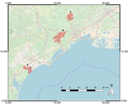
Three study site located in the south of France were involved in our study: (A) Lower Aude Valley, (B)
Mountain of the Moure and Causses of Aumelas and (C) Pic Saint Loup. Figure 1 shows the geographical
position of these three sites. A. Lower Aude Valley
100
The Lower Aude valley (Fig 2(a)) is a Natura 2000 site located in the terminal section of the Aude River. Before reaching the Mediterranean Sea, the Aude River runs through a flat wetland area of about 4 842 ha. From a biodiversity point of view, 56% of the site is composed of Natural Habitat types of Community Interest (NHCI). In total, 19 NHCI are located on the site, including 5 priority habitat types. The most widespread habitats are Mediterranean saltmarshes and Saline coastal lagoons. The
105
remaining area (43.7%) is principally composed of vineyards, cereal crops and temporary or permanent meadows. One more characteristic of the site is its exposure to flooding events (mostly during winter) as well as to drought episodes (maximum intensity occurring in the end of summer). The floodable areas are situated predominantly around the two coastal lagoons: Vendres in the north part of the site and Pisse-Vaches in the south. The Mediterranean sea also influences the salinity across the site
110
(soils and water bodies), with a general gradient increasing from northwest to southeast. B. Mountain of the Moure and Causses of Aumelas
The Mountain of the Moure and Causses of Aumelas (MMCA) (Fig 2(b)) is located at the west of Montpellier (France). Considered as a Natura 2000 site, it has a surface of around 9 369 ha and it is
A
B C
Figure 1: Location of the selected study sites ((A) Lower Aude Valley; (B) Mountain of the Moure and Causses of Aumelas; (C) Pic Saint Loup Natura 2000 site).
.
(a) (b) (c)
Figure 2: Location of the (a) Lower Aude Valley, (b)Mountain of the Moure and Causses of Aumelas and (c) Pic Saint Loup.
situated between 3 basins: the agglomeration of Montpellier, the Thau basin and the Herault valley.
115
Agricultural activities (particularly pastoral activity), fires and rural character of the site make it the largest garrigue territory of the Herault department. This site is characterised by the predominance of natural areas and open habitats. Forests cover its upper part, while the middle is dominated by garrigue vegetation, as for as the south which is characterized by agricultural areas. The MMCA site includes also numerous Mediterranean ponds that are spread over it.
120
C. Pic Saint Loup
Located 20 kilometers north from the city of Montpellier (France), Pic Saint Loup (Fig 2(c)) is a Natura 2000 site. It has a surface around 4 420 ha and covers 8 municipalities: Cazevieille, Mas de Londres, Notre Dame de Londres, Rouet, Saint Jean de Cuculles, Saint Martin de Londres, Saint
125
Mathieu de Treviers and Valflaunes. The Pic Saint Loup site presents a mosaic of land cover classes which includes expanses of lawns and matorrals, rock scarps, forest, cultivated plains, etc. The lawns
are covered by different plants as gagea granatelli/lacaitae. Forest is characterised by green oak, especially in the southern part of the site which is marked by the Mediterranean influences. Note also that human activity such as pastoralism, tree cutting and wood exploitation have greatly contributed
130
to the current landscape.
To perform an inter-site analysis on the three sites described bellow, we exploit satellite images of different sensors: Spot-2, Spot-4 and Spot-5. These satellite images are available in the context of the Spot World
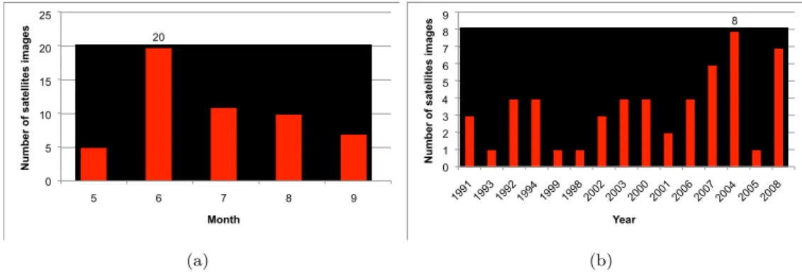
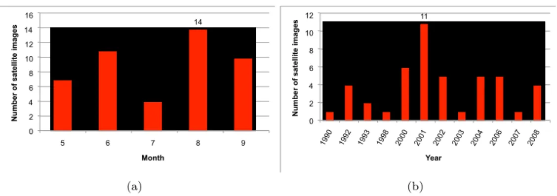
Heritage program (SWH)1. Such images are filtered with the aim to select cloud-free images. We construct
an image dataset composed of three satellite image time series : 53 images for the Lower Aude Valley area,
135
46 images for the MMCA site and 50 images depicting the Pic Saint Loup area. The selected images span over a period of eighteen years, from 1990 to 2008, considering each year the interval between May and September. The dataset description is reported in the table 1.
Spot-2 Spot-4 Spot-5 Total
Lower Aude Valley 29 16 8 53
MMCA 21 17 8 46
Pic Saint Loup 25 17 8 50
Total 75 50 24 149
Table 1: The number of satellite images acquired for each study area per sensor (Spot-2, Spot-4 and Spot-5). The number of satellite images acquired per year and per month on the Lower Aude Valley, MMCA and the Pic Saint Loup sites is illustrated in Figures 3, 4 and 5 respectively.
140 5 20 11 10 7 0 5 10 15 20 25 5 6 7 8 9
Number of satellites images
Month (a) 3 1 4 4 1 1 3 4 4 2 4 6 8 1 7 0 1 2 3 4 5 6 7 8 9 1991 1993 1992 1994 1999 1998 2002 2003 2000 2001 2006 2007 2004 2005 2008
Number of satellites images
Year (b)
Figure 3: The number of satellite images acquired per month (a) and per year (b) on the Lower Aude Valley
2.2. Data Preprocessing
In the preprocessing step, the images are first filtered. The cloudy images are identified and removed from the dataset, then resampled. The resampling process consists on modifying the image resolution by either increasing (oversampling) or decreasing (subsampling) it. In our case, all the images were resampled to 20 meters using the bilinear interpolation method. The objective is to create an homogeneous satellite image
145
dataset. In fact, we use images of different sensors: Spot-2 and Spot-4 provide images with a resolution of 20 meters, while Spot-5 supplies images with a resolution of 10 meters. Next, radiometric information is extracted from satellite images. Successively, a segmentation is performed on them. Finally, a field expert categorize the resulting segments.
1The associate satellite images are available for the research community: https://www.theia-land.fr/fr/projets/spot-world-heritage
7 11 4 14 10 0 2 4 6 8 10 12 14 16 5 6 7 8 9
Number of satellite images
Month (a) 1 4 2 1 6 11 5 1 5 5 1 4 0 2 4 6 8 10 12 1990 1992 1993 1998 2000 2001 2002 2003 2004 2006 2007 2008
Number of satellite images
Year (b)
Figure 4: The number of satellite images acquired per month (a) and per year (b) on the MMCA
9 13 3 15 10 0 2 4 6 8 10 12 14 16 5 6 7 8 9
Number of satellites images
Month (a) 1 3 2 1 1 1 11 9 5 1 5 5 1 4 0 2 4 6 8 10 12 1990 1992 1993 1995 1998 1999 2000 2001 2002 2003 2004 2006 2007 2008
Number of satellites images
Year (b)
Figure 5: The number of satellite images acquired per month (a) and per year (b) on the Pic Saint Loup
2.2.1. Extraction of the Radiometric Information
150
In our study, we use two types of radiometric information: (i) the spectral bands and (ii) the spectral indices. To have a compatible dataset, we keep the common spectral bands on the Spot satellite images: Red, Green and Near InfraRed (NIR). These raw bands are enriched with spectral indices. In this work we compute five spectral indices compatible with Spot satellite images.
• The Soil-Adjusted Vegetation Index (SAVI): Involving two spectral bands, red and NIR, the SAVI [24]
155
index is useful to detect soil and vegetation. It allows to normalize soil variation (dark soil, light soil) avoiding to influence the vegetation spectral response.
• The Brightness Index (BI): The importance of this index appears principally in its potential to show the different situations of soils, by representing their different reflectance and brightness. In fact, beaches and parking lots take the highest value while water area and wet area take the lowest values
160
whereas, agriculture plot shows average values.
• The Color index (CI): The CI [25] index characterises the soil, it is computed using the green and red channels. In most cases, CI gives complementary information with the BI and the NDVI indices for a better understanding of the soil surfaces evolution.
• The Normalized Difference Water Index II: The NDWI2 [26] uses the green and the NIR bands. It
165
allows to characterise the wet and water areas on remote sensing images.
• The Normalized Difference Vegetation Index: The NDVI [27] aims to characterize the vegetation
cover. It ranges in the interval [−1, 1], 1 stands for vegetation canopy, while 0 stands for bare soil. It
Table 2: The segmentation parameters of the three study areas.
Lower Aude Valley Aumelas Pic Saint Loup
Spatial radius 10 20 15
Range radius 5 7 5
Minimum object size 250 250 200
The choice of these spectral indices have been suggested by field experts with regard to the spectral
170
bands provided by the Spot satellites and the characteristic of the study areas. In fact the three sites are characterized by the predomination of the vegetation canopy (in dense form like Forest or less dense like Crop and shrubby vegetation ) and the wet land. Thus, the SAVI, CI, and NDVI are introduced to discriminate different canopy vegetation types, while the BI and the NDWI2 are used to characterize wet lands.
2.3. Segmentation
175
The image segmentation is the process of partitioning an image into segments standing for meaningful structure of the landscape. Each segment groups similar pixels with respect to their radiometric information, while adjacent regions are significantly different with respect to the same characteristics. The goal of the segmentation is to produce a new representation of the image, more significant to analyse.
In this work, the segmentation process is based on four features: the three spectral bands (red, green
180
and near infrared) and the NDVI index. It is performed using the Mean Shift [28] algorithm, which is well adapted to remote sensing image segmentation and especially for high spatial resolution images [29]. In fact, Mean Shift does not make assumption about the number of region or the shape of the region which makes it ideal for handling region of arbitrary shape.
This segmentation algorithm defines a window around each pixel and computes its mean. Then it shifts
185
the center of the window to the computed mean. This algorithm is repeated until it convergences. After each iteration, the window is shifted to a denser region of the image. It involves three parameters: spatial radius, range radius and minimum object size. The spatial radius defines the size of the neighbourhood (window around the pixel), the range radius represents a threshold for the radiometric similarity between the pixels and the minimum object size is used to merge small objects with their neighbour objects. We
190
varied these parameters on each study area. The selected values are reported in Table 2. We stress on the fact that the number of segments is not the same for all the images of the time series. The segmentation step processes each satellite image independently. The image segmentation aims to detect the landscape units of each image.
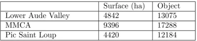
Table 3 reports the number of segments/objects resulting from the image segmentation step. Note that
195
the Lower Aude Valley appears more heterogeneous regarding the total number of segments. While, the number of objects identified on the MMCA site reflects the size of this site and not the heterogeneity of the land cover. The Pic Saint Loup site presents homogeneous land cover, in fact despite the finer segmentation parameters the number of it objects is always the lowest one.
Surface (ha) Object
Lower Aude Valley 4842 13075
MMCA 9396 17288
Pic Saint Loup 4420 12184
Table 3: The surface of the three sites and the number of objects resulting from the segmentation of each SITS . Different segmentation parameters are used for each study area, thus to identify the landscape unit of
200
each site. Our objective is to define compact segments that represent the different entities of the area such us the agriculture plots, forest, etc. The field expert validate the segmentation results by photo interpretation.
2.4. Ground Truth Data
The satellite images are analysed by a field expert to identify their different land cover classes. Observing the three sites (Lower Aude Valley, MMCA and Pic Saint Loup), the expert defines 9 classes. As showed
205
in Figure 6, the three sites have in common 3 classes: Crop, Shrubby vegetation and Vineyard. Therefore, the two sites Pic Saint loup and MMCA have two shared classes: Open space with few or no vegetation and
Forest. While the class Artificial area is specific to the Pic Saint Loup site, the land cover classes : Beach,
Water area and Wet area only appear in the Lower Aude valley site.
The land cover classes repartition in the three study areas is shown in Figure 7. The Pic Saint Loup and
210
the MMCA are mainly characterized by natural habitats as Forest and Shrubby vegetation while, the Lower
Aude Valley by agricultural plots (Crop and Vineyard ), wetlands (Water area and Wet area).
• Artificialised area
• Beach
• Water area
• Wet area • Crop
• Shrubby vegetation • Vineyard
Pic Saint Loup Lower Aude Valley
MMCA • Open space with few or no vegetation
• Forest
Figure 6: The identified land cover classes in the three sites. The classes in common in the study areas are: Crop, Shrubby vegetation and Vineyard.
3. Method
In this section, firstly we supply a general overview of our approach, then we detail the different steps of the proposed framework.
215
3.1. Workflow
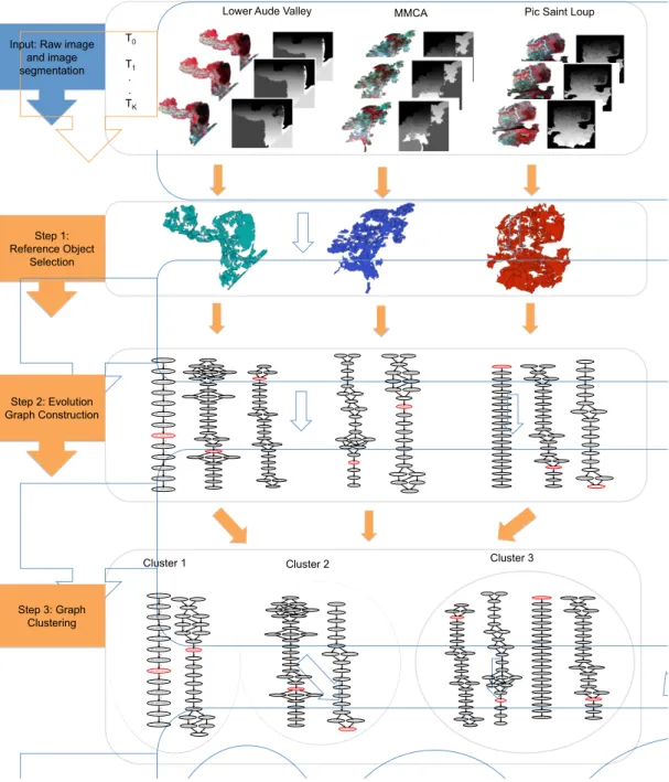
Figure 8 visually summarizes the different steps of the methodology. The framework takes as inputs the raw satellite image time series and its segmentation (Fig 8 (Input)). First, the segments are filtered to detect a subset of objects, named reference objects (Fig 8 (Step 1)). The reference objects stand for the pertinent spatio-temporal entities to analyse. Then, for each reference object, an evolution graph (Fig 8 (Step 2))
220
is built using the segments overlapping it in the SITS. The evolution graph describes the behaviour of the reference object over the time. The graph construction procedure is performed for all the detected reference objects. Finally, a clustering algorithm is applied to detect similar behaviour among evolution
graphs (Fig 8 (Step 3)).
The two first steps of our framework are inspired by the method proposed in [15]. In their work, the
225
authors deploy the strategy on annual time series. Our goal is the analysis of multi-annual SITS data, to this purpose we extend such approach to fit our context.
Figure 7: The repartition of the land cover classes in the three sites. The classes in common in the study areas are: Crop, Shrubby vegetation and Vineyard.
3.2. Preliminaries and Notations
For each study area, we consider a satellite images time series covering the area. A SITS is defined as
an ordered set of satellite images covering the same area, (I1, I2, ... , It, It+1, ... , IT), where the order
230
depends on the acquisition timestamps (1, 2, ..., t, t + 1, ..., T ) of the images.
In addition to raw satellite image time series, we consider also their segmentation. We define for each
image It a set of segment/object, Ot={oit}|Oi=1t|, where i denotes the segment identifier. We associate also
to each object, oi
t, a set of pixels it covers, P ix(oit), and a vector of its radiometric information, Inf o(oit). As the images are segmented independently, each image has a different number of segments. We note
235
withO the union of all the identified segments in the SITS, O =STt=1Ot.
3.3. Reference Object Selection
The first step of the framework is the selection of reference objects [15]. The reference objects are segments standing for phenomena of interest we want to track (spatio-temporal entities). A reference object can be for example an agriculture parcel, in this case the dynamic to track is the growing cycle of the
240
plantations.
At this step, the method analyses the entire set of segments resulting from the satellite images time series segmentation and selects informative objects covering the whole study area.
The intuition behind the reference object selection is the identification of the maximal extent of a certain phenomenon. Thus, we made the assumption that a phenomenon has a dynamic that results on different
245
spatial extent in term of size (the number of pixel covered). This phenomenon reaches its maximal extent at a certain timestamps at least once over the considered period. For instance, if we consider a temporary lake, the lake covers the biggest area over the year in winter. While, during the other seasons (especially in summer) the water will cover a smaller area. Thus, the covered area in winter will be segmented into different objects. The reference object, in this case, is the segment associated to the area covered in winter
250
which corresponds to the maximal extent of the lake. For this reason, the reference object selection step attempts to select the biggest (non overlapping) segments in the satellite image time series.
1_19920507SPOT2 1_19920924SPOT2 1.0 1_19930706SPOT2 1.0 1_19990601SPOT4 1_20000502SPOT2 1.0 1_20000727SPOT4 1.0 1_20070831SPOT4 1_20080621SPOT5 1.0 1_20080821SPOT5 1.0 1_20010801SPOT2 1_20020805SPOT2 1.0 1_20030918SPOT5 1.0 1_20060807SPOT2 1.0 1_19900603SPOT2 1.0 1_20010601SPOT2 1.0 1_20040822SPOT5 1_20060603SPOT5 1.0 1.0 1_20040509SPOT5 1.0 1.0 1_19980906SPOT2 1.0 1_19950529SPOT2 1.0 1.0 1.0 104_20000811SPOT4 181_20010827SPOT2 0.02 371_20020626SPOT2 0.4 213_20000811SPOT4 0.71 410_19910614SPOT2 130_19920516SPOT2 0.55 64_19920516SPOT2 0.29 79_19920813SPOT2 0.3 0.32 787_19930616SPOT2 0.89 130_19980906SPOT2 527_19990618SPOT4 0.29 0.4 0.33 548_20080823SPOT4 63_20020916SPOT2 0.27 488_20080612SPOT4 0.29 596_20080612SPOT4 0.35 63_20070810SPOT4 0.480.7 490_20030607SPOT5 332_20040516SPOT4 0.25 488_20040516SPOT4 0.77 396_20040705SPOT5 0.340.48 0.48 355_20060608SPOT5 799_20070619SPOT4 0.72 0.38 483_19940514SPOT2 239_19940727SPOT2 0.46 0.3 480_20050829SPOT2 0.89 0.44 0.73 12721_20020701SPOT2 17823_20030729SPOT5 0.52 23101_20030919SPOT5 0.98 18051_20030919SPOT5 0.75 13888_19910614SPOT2 10069_19920516SPOT2 0.46 12043_19920516SPOT2 0.59 11352_19920813SPOT2 0.59 14527_19920813SPOT2 0.19 13845_19920813SPOT2 0.16 0.090.45 0.28 14133_20070619SPOT4 19345_20070810SPOT4 0.22 20090_20080612SPOT4 0.8 18943_20080823SPOT4 24473_20060608SPOT5 0.28 12984_20000622SPOT2 15139_20000828SPOT4 0.13 13328_20010626SPOT2 0.25 17958_19990618SPOT4 0.03 0.3 12209_20040706SPOT5 13439_20050829SPOT2 0.88 16177_20050829SPOT2 0.76 12386_20050829SPOT2 0.83 0.47 0.21 0.17 19069_20040516SPOT4 0.29 0.43 0.3 13976_19940817SPOT2 9954_19980906SPOT2 0.14 14817_19980906SPOT2 0.33 16274_19980906SPOT2 0.55 0.060.5 0.2 13497_19930616SPOT2 0.44 12908_19930616SPOT2 0.06 0.0 0.450.240.13 18663_19940624SPOT2 0.07 0.29 0.52 0.4
Lower Aude Valley MMCA Pic Saint Loup
Cluster 1 Cluster 2 Cluster 3
Input: Raw image and image segmentation Step 1: Reference Object Selection Step 2: Evolution Graph Construction Step 3: Graph Clustering T0 T1 . . TK 163_20070831SPOT4 35_20080621SPOT5 0.73 178_20080821SPOT5 0.75 16_20070831SPOT4 0.25 2_20080621SPOT5 0.44 0.01 20_20010801SPOT2 40_20020805SPOT2 0.98 277_20030918SPOT5 0.88 27_19900603SPOT2 29_19920516SPOT2 0.89 2_19920924SPOT2 0.31 50_19920924SPOT2 0.33 2_19900603SPOT2 0.02 26_20040822SPOT5 25_20060807SPOT2 0.17 0.57 0.35 2_19980906SPOT2 2_20000601SPOT4 0.64 2_20000828SPOT4 0.51 141_19980906SPOT2 0.33 2_20040509SPOT5 0.31 0.14 8_20010601SPOT2 0.94 0.68 58_19930806SPOT2 0.03 2_19930806SPOT2 0.82 0.9 0.02 0.83 0.49 28667_20040627SPOT2 75985_20040822SPOT5 0.28 74964_20040822SPOT5 0.44 48724_20060614SPOT4 0.53 0.39 28311_20040627SPOT2 0.16 0.41 28715_20040627SPOT2 0.43 0.07 54742_20070831SPOT4 60818_20080621SPOT5 0.74 72004_20080821SPOT5 0.39 70_20060822SPOT2 0.93 54995_20010927SPOT4 44077_20020915SPOT4 0.74 87235_20030918SPOT5 0.89 0.56 30762_19900603SPOT2 26911_19920516SPOT2 0.01 28040_19920924SPOT2 0.95 31780_19900603SPOT2 0.67 35075_20000602SPOT2 42334_20000828SPOT4 0.82 33845_20010727SPOT4 0.25 34443_20010727SPOT4 0.93 34431_20000602SPOT2 0.01 49926_19980906SPOT2 0.760.18 0.290.8 0.13 0.230.76 37760_19930806SPOT2 0.95 0.77 35_19990601SPOT4 36_20000602SPOT2 0.79 17_20000823SPOT2 0.58 444_20070831SPOT4 9_20080621SPOT5 0.45 588_20080821SPOT5 0.6 394_20060614SPOT4 38_20060822SPOT2 0.48 1.0 10_20060614SPOT4 0.33 394_20010605SPOT4 0.49 33_20010903SPOT2 0.58 574_19900603SPOT2 35_19920516SPOT2 0.47 364_19920924SPOT2 0.65 28_19920924SPOT2 0.98 21_19900603SPOT2 0.4 46_20040822SPOT5 0.62 0.98 38_20040523SPOT2 0.42 948_20030918SPOT5 0.45 561_20020916SPOT4 0.68 280_20020916SPOT4 0.63 443_19980906SPOT2 0.73 646_19950529SPOT2 0.63 25_19930806SPOT2 0.53 0.35 0.48 0.13 0.94 343_20040627SPOT2 589_20040822SPOT5 0.93 510_20060614SPOT4 0.65 377_19990601SPOT4 393_20000602SPOT2 0.91 499_20000828SPOT4 0.32 219_20000828SPOT4 0.62 443_20070831SPOT4 541_20080621SPOT5 0.4 4334_20080621SPOT5 0.47 587_20080821SPOT5 0.55 0.27 482_20060905SPOT4 0.97 0.46 323_19900603SPOT2 1429_19920516SPOT2 0.76 458_19950529SPOT2 0.47 426_20010827SPOT4 0.08 0.87 366_20020916SPOT4 0.61 0.96 442_19980906SPOT2 0.34 0.57 5127_20070831SPOT4 6183_20080621SPOT5 0.74 5917_20060614SPOT4 4582_20060807SPOT2 0.72 0.82 3550_20000823SPOT2 4416_20010612SPOT2 0.92 4480_20010827SPOT4 0.54 2557_19900603SPOT2 1993_19930806SPOT2 0.44 4620_20000602SPOT2 0.92 0.62 6330_20040822SPOT5 0.93 5100_20020915SPOT4 0.84 2445_20040523SPOT2 0.27 0.92 5127_20070831SPOT4 6183_20080621SPOT5 0.74 5917_20060614SPOT4 4582_20060807SPOT2 0.72 0.82 3550_20000823SPOT2 4416_20010612SPOT2 0.92 4480_20010827SPOT4 0.54 2557_19900603SPOT2 1993_19930806SPOT2 0.44 4620_20000602SPOT2 0.92 0.62 6330_20040822SPOT5 0.93 5100_20020915SPOT4 0.84 2445_20040523SPOT2 0.27 0.92 163_20070831SPOT4 35_20080621SPOT5 0.73 178_20080821SPOT5 0.75 16_20070831SPOT4 0.25 2_20080621SPOT5 0.44 0.01 20_20010801SPOT2 40_20020805SPOT2 0.98 277_20030918SPOT5 0.88 27_19900603SPOT2 29_19920516SPOT2 0.89 2_19920924SPOT2 0.31 50_19920924SPOT2 0.33 2_19900603SPOT2 0.02 26_20040822SPOT5 25_20060807SPOT2 0.17 0.57 0.35 2_19980906SPOT2 2_20000601SPOT4 0.64 2_20000828SPOT4 0.51 141_19980906SPOT2 0.33 2_20040509SPOT5 0.31 0.14 8_20010601SPOT2 0.94 0.68 58_19930806SPOT2 0.03 2_19930806SPOT2 0.82 0.9 0.020.83 0.49 28667_20040627SPOT2 75985_20040822SPOT5 0.28 74964_20040822SPOT5 0.44 48724_20060614SPOT4 0.53 0.39 28311_20040627SPOT2 0.16 0.41 28715_20040627SPOT2 0.43 0.07 54742_20070831SPOT4 60818_20080621SPOT5 0.74 72004_20080821SPOT5 0.39 70_20060822SPOT2 0.93 54995_20010927SPOT4 44077_20020915SPOT4 0.74 87235_20030918SPOT5 0.89 0.56 30762_19900603SPOT2 26911_19920516SPOT2 0.01 28040_19920924SPOT2 0.95 31780_19900603SPOT2 0.67 35075_20000602SPOT2 42334_20000828SPOT4 0.82 33845_20010727SPOT4 0.25 34443_20010727SPOT4 0.93 34431_20000602SPOT2 0.01 49926_19980906SPOT2 0.76 0.18 0.290.8 0.13 0.230.76 37760_19930806SPOT2 0.95 0.77 12721_20020701SPOT2 17823_20030729SPOT5 0.52 23101_20030919SPOT5 0.98 18051_20030919SPOT5 0.75 13888_19910614SPOT2 10069_19920516SPOT2 0.46 12043_19920516SPOT2 0.59 11352_19920813SPOT2 0.59 14527_19920813SPOT2 0.19 13845_19920813SPOT2 0.16 0.090.45 0.28 14133_20070619SPOT4 19345_20070810SPOT4 0.22 20090_20080612SPOT4 0.8 18943_20080823SPOT4 24473_20060608SPOT5 0.28 12984_20000622SPOT2 15139_20000828SPOT4 0.13 13328_20010626SPOT2 0.25 17958_19990618SPOT4 0.03 0.3 12209_20040706SPOT5 13439_20050829SPOT2 0.88 16177_20050829SPOT2 0.76 12386_20050829SPOT2 0.83 0.47 0.21 0.17 19069_20040516SPOT4 0.29 0.43 0.3 13976_19940817SPOT2 9954_19980906SPOT2 0.14 14817_19980906SPOT2 0.33 16274_19980906SPOT2 0.55 0.060.5 0.2 13497_19930616SPOT2 0.44 12908_19930616SPOT2 0.06 0.0 0.450.240.13 18663_19940624SPOT2 0.07 0.29 0.52 0.4 343_20040627SPOT2 589_20040822SPOT5 0.93 510_20060614SPOT4 0.65 377_19990601SPOT4 393_20000602SPOT2 0.91 499_20000828SPOT4 0.32 219_20000828SPOT4 0.62 443_20070831SPOT4 541_20080621SPOT5 0.4 4334_20080621SPOT5 0.47 587_20080821SPOT5 0.55 0.27 482_20060905SPOT4 0.97 0.46 323_19900603SPOT2 1429_19920516SPOT2 0.76 458_19950529SPOT2 0.47 426_20010827SPOT4 0.08 0.87 366_20020916SPOT4 0.61 0.96 442_19980906SPOT2 0.34 0.57 104_20000811SPOT4 181_20010827SPOT2 0.02 371_20020626SPOT2 0.4 213_20000811SPOT4 0.71 410_19910614SPOT2 130_19920516SPOT2 0.55 64_19920516SPOT2 0.29 79_19920813SPOT2 0.3 0.32 787_19930616SPOT2 0.89 130_19980906SPOT2 527_19990618SPOT4 0.29 0.4 0.33 548_20080823SPOT4 63_20020916SPOT2 0.27 488_20080612SPOT4 0.29 596_20080612SPOT4 0.35 63_20070810SPOT4 0.48 0.7 490_20030607SPOT5 332_20040516SPOT4 0.25 488_20040516SPOT4 0.77 396_20040705SPOT5 0.340.48 0.48 355_20060608SPOT5 799_20070619SPOT4 0.72 0.38 483_19940514SPOT2 239_19940727SPOT2 0.46 0.3 480_20050829SPOT2 0.89 0.44 0.73 1_19920507SPOT2 1_19920924SPOT2 1.0 1_19930706SPOT2 1.0 1_19990601SPOT4 1_20000502SPOT2 1.0 1_20000727SPOT4 1.0 1_20070831SPOT4 1_20080621SPOT5 1.0 1_20080821SPOT5 1.0 1_20010801SPOT2 1_20020805SPOT2 1.0 1_20030918SPOT5 1.0 1_20060807SPOT2 1.0 1_19900603SPOT2 1.0 1_20010601SPOT2 1.0 1_20040822SPOT5 1_20060603SPOT5 1.0 1.0 1_20040509SPOT5 1.0 1.0 1_19980906SPOT2 1.0 1_19950529SPOT2 1.0 1.0 1.0 35_19990601SPOT4 36_20000602SPOT2 0.79 17_20000823SPOT2 0.58 444_20070831SPOT4 9_20080621SPOT5 0.45 588_20080821SPOT5 0.6 394_20060614SPOT4 38_20060822SPOT2 0.48 1.0 10_20060614SPOT4 0.33 394_20010605SPOT4 0.49 33_20010903SPOT2 0.58 574_19900603SPOT2 35_19920516SPOT2 0.47 364_19920924SPOT2 0.65 28_19920924SPOT2 0.98 21_19900603SPOT2 0.4 46_20040822SPOT5 0.62 0.98 38_20040523SPOT2 0.42 948_20030918SPOT5 0.45 561_20020916SPOT4 0.68 280_20020916SPOT4 0.63 443_19980906SPOT2 0.73 646_19950529SPOT2 0.63 25_19930806SPOT2 0.53 0.35 0.48 0.13 0.94
Figure 8: Overview of the proposed framework to detect and cluster the evolution graphs: (Step1) Reference Object Selection, (Step2) Evolution Graph Construction and (Step3) Graph Clustering .
The reference object selection is treated as a covering problem [15]. We select the subset of segments that cover as much as possible the study area while minimizing their overlapping. In fact, the T images composing the time series cover the same area (the same grid of pixel), a pixel is then covered by T segments.
255
Thus, the selected objects may overlap.
More in detail, the method iterates over the set of segments O, starting from an empty set of reference objects R. At each iteration it selects one object from O and adds it to R. Following the previous main assumption, the method selects the biggest object in the time series. To identify these objects, the segments are weighted. The weight is supplied by the following function:
260 weight(o) = |P ix(o)|, if N ovelty(o) = 1 N ovelty(o), if α < N ovelty(o) < 1 0, if N ovelty(o) < α (1) Where:
• Pix(o) is the set of pixels covered by the segment o
• Novelty(o) is the rate of pixels covered only by the segment o considering the set of objects R. • α is a threshold that defines the minimum value of Novelty a segment must exhibit to be considered. Given a segment o, its weight is equal to the number of pixels it covers, if it does not overlap the objects
265
in R (o does not cover pixels already covered by a selected object in R ). Otherwise (the pixels covered by the segment o overlap with pixels covered by the objects in R), the weight of o is equal to its N ovelty. The N ovelty estimates the contribution of the segment to the coverage of the site considering the current set of selected objects in R. It is computed as follows:
N ovelty(o) = |P ix(o) − P ix(R)|
|P ix(o)| Where:
270
• Pix(o) is the set of pixel covered by the segment o • Pix(R) is the set of pixel covered by the objects in R
To sum up, the method starts by selecting all the non overlapping biggest segments in O (the object having the N ovelty equals to 1), then selecting the segments with the highest N ovelty value in order to cover as much as possible the study area. The parameter α is a threshold ranging between 0 and 1, it allows
275
to fix the minimum N ovelty that a segment should exhibit to be included in R. Hence, this parameter allows to control the rate of the overlapping between the objects in R. The process stops when the weights of all the remaining segments are equal to 0 (their novelty values are lower than the parameter α) or the whole study site is covered. The result is a set of reference objects representing the spatio-temporal phenomena to track.
280
3.4. Graph Construction
In this step, a graph-based representation, called evolution graph, is employed to describe the dynamic of the selected reference objects. An evolution graph is a directed acyclic graph. For each reference object,
o∗, we construct an evolution graph, named G(o∗), defined by a set of nodes (V
o∗) and a set of edges (Eo∗),
Go∗ = (Vo∗, Eo∗). 285
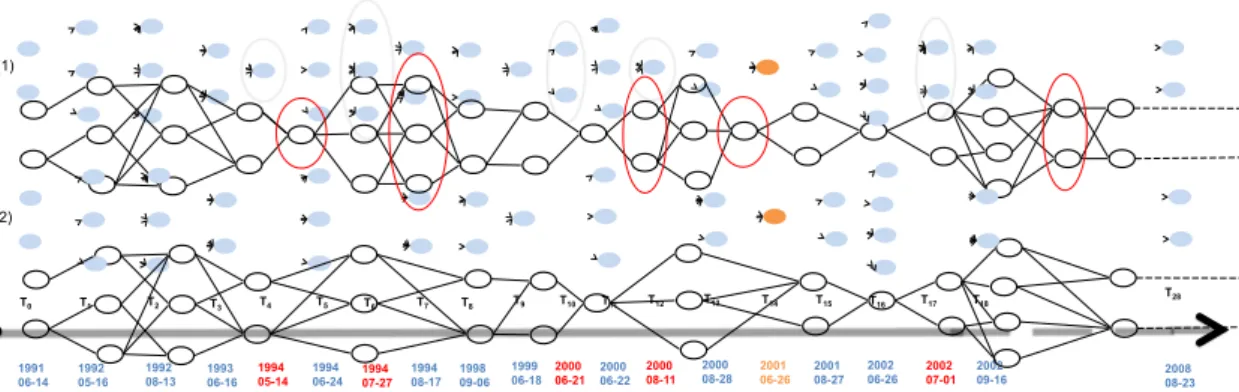
The idea is to track the state of a reference object, o∗, considering the set of satellite composing the
time series. Therefore, the spatial extent of the reference object is projected on the satellite images and its overlapping segments are selected i.e. a group of segments covering the same pixels as the reference object is selected on each image.
In the work proposed in [15], the authors employ the full set of images belonging to the time series
290
in order to derive the corresponding evolution graphs. This was done since the considered time series is short (only six dates) and the goal was to perform phenological analysis. Conversely, in our context we are interested to mine evolution graphs from multi-annual time series. Due to this fact, using all the images of the time series may introduce redundancy, since the difference between the acquisition timestamp of some images is neglectable (i.e. considering the MMCA site: 21-08-2001, 22-08-2001 and 27-08-2001).
295
To deal with this fact, in order to highlight useful evolutions in the land cover reducing redundancy in the information described by the evolution graphs, we need to discard too similar images (according to their date of acquisition). According with field expert recommendations, we set up a time gap of two months between two successive images. Starting from the reference object time stamps, we choose satellite images that are far away (considering the date of acquisition) of at least two months from the previous date of the
300
series.
Considering the spatial extent, the segments to consider, in the evolution graph construction, are those having most of their extent included in the extent of the reference object. The objective is to avoid as much
as possible the noisy segments and the non-representative ones. Therefore two thresholds are defined, σ1
and σ2: 305 Vo∗ ={o|o ∈ O,|P ix(o ∗)∩ P ix(o)| |P ix(o)| ≥ σ1 or |P ix(o∗)∩ P ix(o)| |P ix(o∗)| ≥ σ2} Where:
• O is the set of segment • o is a segment on O
• o∗ is a reference object
• P ix(o) is the set of pixels covered by the segment o
310
• P ix(o∗) is the set of pixels covered by the reference object o∗
The first parameter (σ1) is the most significant and allows the selection of segments that should present
most of their spatial extent inside the reference object extent. The second parameter (σ2) is used to retain
all the objects covering more than a certain percentage of the reference object extent.
Once the representatives segments of the reference object are selected, they are organized and linked
315
to form an evolution graph. The segments are first grouped considering their images timestamps i.e. each group will contain all the segments belonging to the same image of the time series. Then, the segments groups are sorted in increasing order considering the timestamps (acquisition date) of their image. Finally, the segments of each two successive groups are connected by links. To link the segments we consider always their extent linking overlapping ones. Thus, segments belonging to the same image are not linked. We
320
consider also their timestamps, thus segments not belonging to two images with successive timestamp are not linked. Therefore only segments belonging to two successive timestamps are linked forming an acyclic
directed graph. The set of edges, Eo∗, is defined as follows:
Eo∗ ={(oi, oj)|oi∈ Ot∩ Vo∗, oj∈ Ot+1∩ Vo∗, P ix(oi)∩ P ix(oj)6= ∅}
Where:
• Otand Ot+1 are the sets of segments corresponding respectively to the images It and It+1
325
• oi and oj are segments of the images I
tand It+1respectively
• P ix(oi) is the set of pixels covered by the segment oi
2001 06-26 2001 08-27 2002 06-26 2002 07-01 2002 09-16 2000 08-28 2000 08-11 2000 06-22 2000 06-21 1999 06-18 1998 09-06 1994 08-17 1994 06-24 1994 05-14 1994 07-27 1993 06-16 1992 08-13 1992 05-16 1991 06-14 2008 08-23 T14 T15 T16 T17 T18 T13 T12 T11 T10 T9 T8 T7 T5 T4 T6 T3 T2 T1 T0 T28 (2) (1)
Figure 9: Evolution graph example constructed in the Lower Aude Valley using a reference object selected in the satellite image acquired on 26-06-2011.
Figure 9 shows an example of two evolution graphs (1,2) corresponding to the same reference object. The graph (1) is constructed using all the satellite images of the time series while graph (2) is built considering
330
only the images satisfying the time gap constraint of two months between their timestamps.
We can observe that a graph can be organized by timestamps from left to right. The time line contains: the orange timestamp which is that of reference object, the blue timestamps who are those of the considered images in the evolution graph construction step and the red ones standing for the timestamps of the discarded images. The graph (1) points out the discarded timestamps which do not appear on the final evolution
335
graph (2).
Each timestamp in the time line corresponds to a set of segments in the evolution graph. These times-tamps reference to the image in which the segments were identified. As shown in Figure 9, only the segments corresponding to two successive timestamps are linked. Note that, in the evolution graph, segments corre-spond to nodes and links correcorre-spond to edges.
340
3.5. Graph Clustering
The graph clustering involves the transformation of the evolution graphs into synopsis. The synopsis summarize their information and allows us to compute the distance between them. The distance between two
evolution graphs is the distance between their respective synopsis. Considering the distance between each
pair of synopsis, a distance matrix is generated. Using the distance matrix, we apply a clustering algorithm
345
that identifies the different groups among the evolution graphs with the aim to distinguish different evolution behaviours.
Figure 10 summarizes the synopsis generation. A synopsis is defined as a sequence of generated nodes, ( fO1, fO2, ..., fOt, gOt+1, ..., fOT), it contains as many nodes as images used to built the corresponding evolution
graph. Each generated node fOtis obtained by a weighted aggregation of the radiometric values of the nodes
350
with the timestamps t. This radiometric values are computed as follow: Inf o(fOt) =
P
ot∈Vo∗|P ix(ot)| Info(ot)
P
ot∈Vo∗|P ix(ot)|
(2)
The node oi
t in the evolution graph (Figure 10) represents a segment, where t is the image timestamp
and i is the segment identifier. The evolution graph, in Figure 10 is composed of four groups of segments ({{o1
1, o21}, {o12, o22}, {o13}, {o14, o24}}). A synopsis is defined as a sequence of averaged segments, one segments per timestamps (image) i.e., each group of segments in the evolution graph is transformed into one averaged
355
object(( fO1, fO2, fO3, fO4)).
More in detail, the segments of each evolution graph are aggregated per image. They are first weighted by their size to give more importance to bigger segments, then averaged to create only one segment. The segments in the evolution graph are considered as a vector of features (spectral bands and radiometric
O
11O
12O
21O
22O
14O
24O
13,
,
,
f
O
1, , ,
O
f
2O
f
3O
f
4 Evolution graph Segments aggregation Synopsis P i2(1,2)|P ix(o i 2)| ⇤ oi2 P i2(1,2)|P ix(o i 2)| P i2(1,2)|P ix(o i 1)| ⇤ oi1 P i2(1,2)|P ix(o i 1)| P i2(1,2)|P ix(o i 4)| ⇤ oi4 P i2(1,2)|P ix(o i 4)| |P ix(o1 3)| ⇤ o13 |P ix(o1 3)|Figure 10: The procedure to build a synopsis of an evolution graph that aggregates together the set of segments of each satellite image.
indices: green, red, near infared, NDVI, NDWI, BI, CI and SAVI ). Each vector/segment is first weighted
360
by its number of pixels. Then, it is averaged to create new vector/segment.
Once the evolution graphs are transformed into a synopsis. The next step is the distance computation.
The distance is computed for each pair of synopsis. Given two evolution graphs G1 and G2, we define their
corresponding synopsis syn1 and syn2, then we compute the distance between them as following:
dist(syn1, syn2) = DT W (syn1, syn2) (3)
To estimate the distance between the synopsis, we use the Dynamic Time Warping (DTW) distance
365
measure [30]. This distance measure allows to estimate the distance between two time series of different sizes and find their optimal alignment. It is a time-designed distance measure able to gather time-distorted sequences with temporal shifts [31]. Considering these proprieties, DTW is adapted to our study case. In fact, the number of satellite images considered for each site is different due to noisy and missing information (i.e. cloudy images). Therefore, the resulting synopsis can have different lengths. Note also that, for the
370
same study site, the timestamps of evolution graph can differ from each other due to the time gap constraint. Give two time series C = (c1, c2, ...., cn) and Q = (q1, q2, ..., qm), of length n and m respectively (n6= m). To compute the distance between this two time series using the dynamic time warping (DTW) measure, a
matrix D of size n∗ m is constructed as follows:
D(cl, qr) = θ(cl, qr) + min D(cl−1, qr−1) D(cl, qr−1) D(cl−1, qr) Where: 375
• θ is a distance measure (Euclidian distance is the most one used)
The matrix is initialized computing the first element (D(c1, q1)). The other elements are then computed
using the minimum between the left, upper or diagonal one. The distance between the two series is given by the last element:
DT W (C, Q) = D(cn, qm)
Once the distance matrix is obtained using the DTW measure, the clustering step allows gathering
380
the synopsis into homogeneous clusters. Each cluster groups similar synopsis. The clustering process consider the evolution graphs of the different sites and allows discovering similarities among them. The clustering is performed using the hierarchical agglomerative algorithm [32]. This clustering algorithm creates a dendrogram which is a tree-level structure, where each level contains a partition set.
The hierarchical agglomerative algorithm begins with each point in its own cluster and progressively
385
joins the closest clusters until only one cluster remains. Thus, we result in different clustering solutions with different cluster number which allows the expert to choose a clustering solution considering different granularity.
We remind that also in [33] the authors perform evolution graphs clustering but, conversely to them, in our scenario: i) we consider multi-annual time series, ii) we jointly analyse several sites at the same time
390
and iii) we deal with time series with variable length.
3.6. σ1 andσ2 setting
The described approach use three parameters: • α allows to select relevant reference objects.
• σ1and σ2 avoid to associated noisy segments to an evolution graph.
395
The threshold α allows to select a subset of reference objects while minimizing the overlapping among them. The idea is to select segments that cover as much as possible the study area while minimizing the
overlapping. While σ1 and σ2 avoid to select irrelevant segments in the evolution graph construction i.e.,
select only the segments that cover the reference object spatial extent on the time series.
To select the values of the three parameters we consider the coverage and overlapping of the evolution
400
graphs. The evolution graph coverage defines the area covered by all the segments of all the constructed
evolution graphs while, the evolution graphs overlapping defines the area covered by at least two evolution
graphs.
To fix the appropriate parameters values, we varied them in range [0, 1] generating different combina-tions. Then, we use the different combinations to construct the evolution graphs and report their coverage
405
and overlapping. Considering the obtained coverage, we fix a threshold, named τ , for the minimum accept-able coverage. Among the combinations that satisfy the threshold, we select the one with the minimum overlapping rate.
3.7. Validation of the results
Once the reference objects are selected, their evolution are analysed and grouped in different clusters
410
using the Hierarchical Agglomerative Clustering (HAC) algorithm. The clusters involve the graphs evolving similarly. Each cluster highlights a different behaviour pattern.
To evaluate our framework, the evolution graphs are classified by the field expert in nine land cover classes as described in section 2.4. Then, the identified classes are compared to the clustering results using two evaluation measures: the Normalized Mutual Information (NMI) and the Adjusted Rand Index (ARI) [34].
415
To define the NMI and ARI, Lets consider a clustering result C ={C1. . . CJ} with J clusters and an
expert classification P ={P1. . . PI} with I classes. We note n the numbers of entities to analyse.
The NMI is a clustering validity index that measures the information shared between the generated clusters and the identified classes. This metric is independent from the number of clusters and ranges between 0 and 1, the higher the value the more the clustering grouping and the expert classification partition
420
agree. It is computed considering each pair of clusters and classes as follows:
NMI(C, P) = PI i=1 PJ j=1xijlog nxij xixj qPI i=1xilog xi n PJ j=1xjlog xj n (4)
Where:
• xij is the cardinality of the set of entities that belong to cluster Cj and class Pi
• xj is the number of entities in the cluster Cj
• xi is the number of objects in the class Pi
425
The ARI measures the agreement between two partitions by considering all pairs of entities and counting pairs that are assigned in the same or different cluster in two partitioning. We note a the number of entity pairs belonging to the same cluster in C and the same class in P , the ARI is computed using the following equation:
ARI(C, P) = a− E[a]
max(a)− E[a]
Where:
430
• E[a] represents the expectation value of a • max(a) represents the maximum value of a
E[a] and max(a) are computed using the following equations:
E[a] = π(C)· π(P )
n(n− 1)/2
max(a) = 1
2(π(C) + π(P ))
Where:
• π(C) denote the number of object pairs that belong to the same cluster in C
435
• π(P ) denote the number of object pairs that belong to the same class in P
The rand index lies between 0 and 1. When the two partitions agree perfectly, the ARI is equal to 1. The obtained results are reported and discussed in the next section.
4. Experimental Results and Discussion
In this section, we present and discuss the results of our analysis. First, we extract the evolution
440
graphs from the study areas adopting the proposed approach. Then, we perform the clustering analysis on
the evolution graphs obtained from the three study areas . Finally, we present qualitative results on the obtained clusters.
4.1. Parameters Setting
Our framework needs as input three parameters (α, σ1 and σ2 ) that allow us to select informative
445
and non-redundant sets of reference objects from the SITS data. With the aim to choose the parameter combination that maximize the coverage, we vary their range in the interval [0, 1] with a step of 0.1. For each combination, the set of evolution graphs is constructed. Associated to each set of evolution graphs, we can compute the coverage and the overlapping ratio. Figure 11 reports the coverage for the three study sites. We discretize the coverage ratio in bins (the histogram bins range between 0% and 100% with a step
450
of 5% ). Each bin represents how many times a parameter combination produces a set of evolution graphs with that particular coverage.
0 5 10 15 20 25 30 35 40 45 50 55 60 65 70 75 80 85 90 95 100 Graph coverage 0.0 0.1 0.2 0.3 0.4 0.5 0.6 Probability (a) 0 5 10 15 20 25 30 35 40 45 50 55 60 65 70 75 80 85 90 95 100 Graph coverage 0.0 0.1 0.2 0.3 0.4 0.5 0.6 0.7 0.8 0.9 Probability (b) 0 5 10 15 20 25 30 35 40 45 50 55 60 65 70 75 80 85 90 95 100 Graph coverage 0.0 0.1 0.2 0.3 0.4 0.5 0.6 0.7 Probability (c)
Figure 11: The probability of the evolution graphs coverage rate of the three sites: (a) Lower Aude Valley, (b)MMCA and (c) Pic Saint Loup.
Figure 11 reports the evolution graphs coverage for the Lower Aude Valley (Figure 11(a)), the MMCA (Fig-ure 11(b)) and the Pic Saint Loup (Fig(Fig-ure 11(c))
Once the results are analysed, we select 85%, 90%, 90% as coverage threshold for the Lower Aude
455
Valley, the MMCA and the Pic Saint Loup respectively. As observed in Figure11, more than 50% of
the combinations cover more than 95% of the study area, despite that the fixed thresholds are inferior to 95%. This is due to the high overlapping rate of the generated graphs by these combinations. The retained combination generates a set of evolution graphs covering as much as possible the study areas while minimizing the overlapping rate.
460
Using the selected parameters values, we extract 233 reference objects: 67 on the Lower Aude Valley, 87 on the Pic Saint Loup and 79 on the MMCA sites. The selected reference objects result on 233 evolution
graphs covering around 89% of the three study areas. Figure 4 reports the selected parameters values as
well as the coverage and overlapping rate of the resulting evolution graphs.
α σ1 σ2 Evolution graph Evolution graphs coverage Evolution graphs overlapping
Lower Aude Valley 0.5 0.9 0.7 67 88.27 26.02
MMCA 0.4 0.9 0.8 79 90.29 22.71
Pic Saint Loup 0.3 0.9 0.8 87 90.80 30.3
Table 4: The selected parameters values and the numbre of resulting evolution graphs with their coverage and overlapping rate on each study area.
4.2. Clustering Results
465
The generated evolution graphs are grouped with the aim to characterize common behaviour among the different spatio-temporal phenomena. To this end, we use the hierarchical agglomerative clustering with
average linkage. This algorithm creates a hierarchy of partitions with different number of clusters. Among the different level of the hierarchy, we choose the solution that involves 20 clusters.
The clustering algorithm works on the evolution graphs features (the spectral bands and the spectral
470
indices). With the aim to understand the influences of the different feature groups, we cluster the evolution
graphs considering two different scenario: (i) a clustering performed considering only the spectral bands and
(ii) a clustering performed considering both spectral bands and spectral indices.
Figure 12 illustrates the obtained results from the analysis of the evolution graphs using the three spectral bands: Green, Red and Near Infrared. Whereas, figure 13 illustrates the results obtained combining the
475
spectral bands and the spectral indices: NDVI, NDWI, BI, CI and SAVI.
Figure 12: The distribution of the reference objects in the 20 clusters on the three sites using the spectral bands: Green, Red and Near Infrared.
Figure 13: The distribution of the reference objects in the 20 clusters on the three sites using both the spectral bands and the spectral indices: Green, Red, Near Infrared, NDVI, NDWI, BI, CI and SAVI .
For the Lower Aude Valley (Figure 12), the evolutions of the reference objects are grouped in 18 clusters. The Water area class corresponds to the clusters 4, 5 and 18. The class Wet area is represented by the clusters 11 and 13 while the class Beach grouped in the cluster 15. The class
480
Vineyard is also grouped in the clusters 6, 12 and 16, this partitioning in different clusters is explained
by the phenological stage of the observed vineyard. More in detail, depending on the stage of their development, the radiometric values of the vineyards differ, which makes their discrimination possible. However, the clusters 0, 7 and 8 group the different vegetation canopy classes (Vineyard, Shrubby
vegetation and Crop) and the wetland (Water area and Wet area), The cluster 2 groups the aquatic
485
vegetation among the two classes Wet area and Water area. The class Crop is identified on the clusters 3, 14 and 17.
In the second case (Figure 13), the radiometric information allows to distinguish the different classes among the Lower Aude Valley, The class Water area is grouped in the clusters 10, 13 and 4 which stands for the aquatic vegetation. The class Beach is represented by the cluster 15. Also the class
490
Wet area is grouped in the clusters 9 and 17. The vegetation is grouped in the cluster 0 (Crop and
Vineyard). The clusters 2, 6 and 12 group the classes Crop,Vineyard, Wet area and Shrubby vegetation
that show similarities in their radiometric reflectance values on the considered period. B. The Mountain of the Moure and Causses of Aumelas
495
Despite the number of clusters (20), we identified 2 clusters on the MMCA site (Figure 12). The cluster 0 groups the vegetation canopy (Crop, Shrubby vegetation, Vineyard and open space with no or few vegetation). These reference objects evolutions are characterized by high reflectance values in all bands. When the cluster 2 groups the Forest and the Shrubby vegetation classes which are characterised by low reflectance values in the visible bands (Green and Red) and hight values in the
500
Near Infrared.
Considering both spectral bands and the spectral indices, we identify 3 clusters in the MMCA (Fig-ure 13). The cluster 19 is specific to the class Forest, the cluster 4 groups the classes Forest and
Shrubby vegetation. The cluster 7 groups the Vineyard and Shrubby vegetation classes. The NDVI
and SAVI indices allow to identify the density variation of the vegetation canopy.
505
C. Pic Saint Loup
In The Pic Saint Loup, we detect 6 clusters (Figure 12). The class Forest is well discriminate on the clusters 2 and 8. The cluster 18 corresponds also to Forest, however the shaded side of the Pic
Saint Loup mountain affect its radiometric properties. The cluster 1 which groups the vegetation
510
canopy (Crop, Shrubby vegetation and Vineyard ). Cluster 0 groups the class Forest and Shrubby
vegetation which have high reflectance in the NIR band, this fact explains that these two classes are
grouped together.
With the use of the spectral indices, we identified 9 clusters in Pic Saint Loup site (Figure 13). Cluster 2, 3 and 6 group the classes Shubby vegetation and Forest that evolve similarly. The clusters 0, 4 and
515
8 group the Forest class. Regarding classes Crop and Vineyard, they are associated to cluster 1 and 14.
The main objective of this work is to perform an object-oriented analysis on multi-annual SITS data to underline intra and inter-site similarities among the different study areas. To deal with this goal, we have proposed a method to analyse multi-annual SITS data based on a graph representation. To asses the
520
proposed method, we perform analysis on three study areas. As a result, we identify both: spatio-temporal evolutions specific to an area and and spatio-temporal evolution that are shared among different sites.
Considering the clustering performed only on spectral bands (Figure 12), the clusters 0 and 2 group spatio-temporal entities of the three study areas. Those phenomenon show similar temporal behaviours. The cluster 0 groups the vegetation classes. The cluster 2 groups vegetation classes from the MMCA and
the Pic Saint Loup but, it corresponds to Wet area and vegetation classes on the Lower Aude Valley. The
Wet area class is grouped with the vegetation classes because they share a close radiometric response.
Clusters 8 and 18 group together entities of the Pic Saint Loup and the Lower Aude Valley. Cluster 18 corresponds to water on the Lower Aude Valley and shadow areas on the Pic Saint Loup. The grouped phenomenon in cluster 18 have a different radiometric response in the Near Infrared band, but they show
530
similarities in the Red and Green bands. On the other hand, cluster 8 corresponds to vegetation on the two sites, it groups Vineyard, Crop and Wet land objects on the Lower Aude Valley and Forest, Shrubby
vegetation and Crop classes on the Pic Saint Loup.
When combining the spectral bands with the spectral indices (Figure 13), similar phenomenon among
535
the three study areas are grouped together in cluster 4. Cluster 4 corresponds to Forest in the Pic Saint
Loup, it involves Forest and Shrubby vegetation coming from the MCCA site while, for the Lower Aude
Valley, it corresponds to aquatic vegetation (Water area). The fact that these classes are gathered in the
same group is explained by their similarity in the NDVI response.
Regarding the Lower Aude Valley and the Pic Saint Loup, the clusters 2 and 6 group similar
spatio-540
temporal entities together. Cluster 2 corresponds to Forest in the former site and groups the classes: Crop,
Vineyard and Wet area in the latter site. The spatio-temporal entities in the cluster 2 have similar NDVI
and SAVI evolution. Concerning cluster 6, it groups spatio-temporal entities of theShrubby vegetation class on the Pic Saint Loup and Wet area class on the Lower Aude Valley. These two classes are grouped together as they have a similar radiometric evolution considering all the set of bands and indices.
545
To assess the performance of our clustering approach, we compared the clustering result to the classifi-cation supplied by the field expert. We compute the NMI and the ARI between these two partitions. More in detail, we repeat this comparison four times, one for each of the site independently (in the context of intra-site analysis) and once considering the simultaneous clustering of the full set of study areas (in the context of the inter-site analysis). The analysis are performed considering two different configurations: only
550
the raw bands (Figure 12) and the combination of raw bands and radiometric indices (Figure 13). The results are reported in Table 5.
Considering the NMI results, despite some confusion in the Pic Saint Loup, we note that the method performs generally better using the spectral bands combined with the indices than using only the spectral bands. Considering the ARI results, they show that including the spectral indices in the analysis enhances
555
the clustering process excepting for the Lower Aude Valley in which better results are achieved using only the spectral bands.
Spectral bands Spectral bands
and indices
ARI NMI ARI NMI
Lower Aude Valley 0.25 0.258 0.193 0.292
MMCA 0.104 0.151 0.218 0.238
Pic Saint Loup 0.164 0.26 0.223 0.211
Intra-sites 0.152 0.236 0.159 0.246
Table 5: Normalized Mutual Information and Adjusted Rand Index results obtained using: i) the spectral bands ii) the spectral bands plus the radiometric indices on the study areas.
4.3. Evolution Graphs Analysis Results
With the aim to inspect the spatio-temporal evolution extracted by our approach, we report in Figures 14-18 some examples of evolution graphs. Such examples depict representative evolution graphs belonging to
560
cluster 4 and 6.
We avoid to draw the whole evolution graphs since they are composed by more than twenty timestamps. To improve the readability we select only some timestamps (five) for each evolution graph. The colour of the segments represents their radiometric values. Thus, the change of the colours indicates the evolution of
the considered segments. We visualize the satellite images segments in false-colour. Adopting this choice,
565
the vegetation canopy will appear in red.
Figure 17 and Figure 18 show two evolution graphs belonging to the Lower Aude Valley and the Pic Saint
Loup respectively. Both evolution graphs are grouped in cluster 6 and define a reference object covered by
shrubby vegetation. As we know the evolution of shrubby vegetation is progressive and it remains constant most of the time. This is why the colour of the segments remains mostly unchanged in all the timestamps.
570
Figures 14, 15 and 16 show three evolution graphs corresponding to the Lower Aude Valley, the MMCA and the Pic Saint Loup respectively. They are grouped together in cluster 4. The two last evolution graphs (Figure 15 and Figure 16) represent forest areas which are characterized by a dense vegetation canopy, thus the satellite images are characterized by a darkened red colour. In addition, the forest cover is not influenced by seasonal change, thus the radiometric values of those areas remain unchanged. Figure 14 illustrates an
575
evolution graphof a water area covered by aquatic vegetation, the water area appears in darkened blue while
the vegetation appear in red. This combination of radiometric values is quiet similar to the forest cover, thus these three evolution graphs are grouped together.
2000 06-21 1994 07-27 1992 05-05 2007 08-10 2002 09-16
Figure 14: Evolution graph example of the Lower Aude Valley describing the dynamic of a water area covered by aquatic vegetation grouped in the cluster 4.
To sum up, we analysed the clustering results for the three study areas considering only raw images (spectral bands) and spectral bands plus derived spectral indices. When only raw bands are employed, we
580
2001 08-01 1993 08-06 1990 06-03 2007 08-31 2003 09-18
Figure 15: Evolution graph example of the MMCA describing the dynamic of a forest area grouped in the cluster 4.
2000 07-27 1993 07-06 1992 05-16 2008 08-21 2003 09-18
Figure 16: Evolution graph example of the Pic Saint Loup describing the dynamic of a forest area grouped in the cluster 4.
the use of spectral indices induces an improvement of the clustering results.
1993 06-16 1991
06-14 2001 08-27 2003 07-29 2007 08-31
Figure 17: Evolution graph example of the Lower Aude Valley describing the dynamic of an area covered by shrubby vegetation grouped in the cluster 6.
1993 08-06 1990 06-03 2003 09-18 2007 08-31 2001 08-01
Figure 18: Evolution graph example of the Pic Saint Loup describing the dynamic of an area covered by shrubby vegetation grouped in the cluster 6.


![[DOC] Cours JavaScript : Les Tableaux](data:image/gif;base64,R0lGODlhAQABAIAAAP///wAAACH5BAEAAAAALAAAAAABAAEAAAICRAEAOw==)