Aeroacoustics of Perforated Drag Plates
for Quiet Transport Aircraft
by
Kiril Dimitrov Sakaliyski
B.S., Aeronautical Engineering
Technical University-Sofia, 2002
Submitted to the Department of Aeronautics and Astronautics
in partial fulfillment of the requirements for the degree of
Master of Science in Aeronautics and Astronautics
at the
MASSACHUSETTS INSTITUTE OF TECHNOLOGY
September 2005
c
° Massachusetts Institute of Technology 2005. All rights reserved.
Author . . . .
Department of Aeronautics and Astronautics
August 19, 2005
Certified by . . . .
Zoltan Spakovszky
Associate Professor of Aeronautics and Astronautics
Thesis Supervisor
Accepted by . . . .
Jaime Peraire
Professor of Aeronautics and Astronautics
Chairman, Department Committee on Graduate Students
Aeroacoustics of Perforated Drag Plates
for Quiet Transport Aircraft
by
Kiril Dimitrov Sakaliyski
Submitted to the Department of Aeronautics and Astronautics on August 19, 2005, in partial fulfillment of the
requirements for the degree of
Master of Science in Aeronautics and Astronautics
Abstract
Historically aircraft noise is one of the principal environmental issues for aviation. Within this context, the Silent Aircraft Initiative was launched with the objective to achieve a step-change in noise reduction compared to current practice. One of the most critical tasks in noise reduction is to develop technologies to increase drag in quiet ways. The work presented in this thesis focuses primarily on aeroacoustic tests and analysis of perforated drag plates. The idea behind a quiet spoiler or drag rudder is to alter the noise production mechanism by perforating the drag plates. The hypothesis is that the large length scales responsible for the noise radiated by unsteady vortical structures can be changed to small length scales driving jet noise at frequencies which are perceived unannoying by the human ear.
The aeroacoustic characteristics of laboratory-scale perforated spoilers were measured in an acoustic chamber at MIT. Based on the experimental data a noise prediction model was developed for the bluff-body and turbulent mixing noise generated by a perforated drag rudder. Acoustic phased array measurements of seven perforated plates in four different installation configurations were conducted in the Markham wind tunnel at Cambridge University to further investigate the noise mechanisms. The analysis of the test results showed that there are two identifiable peak frequencies which scale with free stream velocity. Different candidate length scales were investigated with the goal to collapse the data on a Strouhal number basis. However, a universal length scale was not found. It was hypothesized that the noise is mainly due to the isotropic turbulence generated behind such perforated plate. Due to the high background noise levels in the experiments the impact of the perforations on the low frequency noise signature could not be assessed.
A perforated plate of 28.19% porosity with a hole diameter to plate length ratio d/L of 0.013 and a non-dimensional hole separation s/L of 0.0217 was identified to be the most beneficial plate in terms of noise reduction. The experiments showed that a spoiler mounted on the suction surface of the wing is the quietest configuration. In order to scale the results to full size, the observed peak magnitudes are suggested to scale with the 4th power
of the free stream velocity. In addition, the overall sound pressure levels were found to scale with plate size such that an increase in source area causes an equivalent increase in the acoustic power.
The developed models were used to predict the noise signature of a full sized drag rudder which enabled a 6◦ glide slope angle resulting in a 4 dBA reduction in cumulative sound pressure level of the candidate SAX10
Silent Aircraft design.
Thesis Supervisor: Zoltan Spakovszky
Acknowledgments
The completion of this thesis is the result of assistance and advice from a number of individuals.
First and most importantly, I want to thank my advisor, Prof. Zoltan Spakovszky, for giving me the opportunity to work on this very interesting project and his support, insight and guidance over the past two years.
Second, I need to thank Dr. James Hileman for answering numerous questions concerning aeroacoustics, providing me with invariable ideas and for always taking time to review and make sense of the test results.
I also wish to thank the following individuals that have made my Gas Turbine Laboratory experience much more memorable: Juan Castiella, Adam Diedrich, Justin Jaworski, Anya Jones, Nayden Kambouchev, Vai-Man Lei, Jean-Francois Onnee, An-gelique Plas, Parthiv Shah, Yuto Shinagawa, Dr. Borislav Sirakov, Ryan Tam, David Tan and Serge Tournier. Thanks to Prof. Edward Greitzer for keeping me busy dur-ing the terms I took his classes, which on the other hand gave me the depth I need to interpret computational results and hence effectively extract conclusions about key features of complex flows.
I would also like to express my thanks to my best friends Mariya Petrova and Olivier Toupet whom I had numerous memorable experiences with while studying for the Ph.D. qualifiers and goofing around on a daily basis.
Special thanks to the people from the Silent Aircraft Initiative and especially the airframe team members Christodoulos Andreou, Andrew Faszer and Ho-Chul Shin for their valuable help and ideas.
The author wishes to gratefully acknowledge the help of Victor Dubrowski, James Letendre and Richard Perdichizzi at MIT and John Clark at Cambridge University for their help with the experiments’ setup and without whom this work would have not been possible. Thanks are due also to Jordan Brayanov and Atanas Pavlov for their help and valuable technical advice throughout the course of this project.
who always encouraged me to pursue my dreams. I could not have gone so far, if there were not their full support.
Last, but not least important, I want to thank my true love Krassi for supporting me through those long days when we are long apart and spent so little time together. This project was part of the Silent Aircraft Initiative and was funded by the Cambridge-MIT Institute. This support is gratefully acknowledged.
Nomenclature
Romand perforation diameter
x horizontal separation between two neighboring perforations or axis direction y vertical separation between two neighboring perforations or axis direction
s separation between two neighboring perforations in a uniform perforation pattern U free stream velocity
a speed of sound
F force
j √−1
f frequency
fs vortex shedding frequency or sample rate
∆f frequency resolution T length of a time signal H height of a plate L length of a plate
r distance to an observer or radius
p pressure
CD drag coefficient
C contraction coefficient
u mean velocity through a perforated plate
D drag force
xs spoiler location on the wing, measured from the wing leading edge
cws wing chord at spoiler location
St Strouhal number
Re Reynolds number
M Mach number
N number of perforations or number of sample points I acoustic intensity
P acoustic power
AIF area increase factor
n exponential speed dependance of the plate noise levels
Greek
β porosity, defined as the ratio of open to total plate area ρ air density
µ air viscosity
θ directivity angle in degrees
κ plate resistance to a passage of air ψ deployment angle of a drag device
ρ density
δ boundary layer thickness ω angular frequency
Subscripts
P P perforated plate or pistonphone quantity SP solid plate quantity
corr corrected quantity
P peak quantity
norm normalized quantity req required quantity prod produced quantity
av average quantity
Abbreviations
SAI Silent Aircraft Initiative
SAX Silent Aircraft eXperimental design MIT Massachusetts Institute of Technology
CU University of Cambridge
FFT Fast Fourier Transform
SPL Sound Pressure Level
OASPL Overall Sound Pressure Level
Contents
1 Introduction 23
1.1 Background . . . 24
1.1.1 Aircraft Noise Sources . . . 24
1.1.2 Silent Aircraft Initiative . . . 26
1.2 The Idea Behind Silent Spoiler/Drag Rudder . . . 29
1.2.1 Research Objectives . . . 30
1.2.2 Research Questions . . . 30
1.2.3 Success Goals . . . 31
1.2.4 Technical Approach . . . 31
1.3 Thesis Outline . . . 32
2 Description of Noise and Drag Mechanisms of Perforated Drag Plates 33 2.1 Noise Mechanisms Associated with Perforated Drag Plates . . . 33
2.2 Dimensional Analysis . . . 35
2.3 Drag Analysis . . . 38
3 MIT Acoustic Chamber Design and Instrumentation 45 3.1 Acoustic Facility Design . . . 46
3.1.1 Microphone Placement . . . 48
3.2 Acoustic Instrumentation . . . 49
3.2.1 Microphone Instrumentation . . . 49
3.2.2 Data Acquisition System . . . 52
3.3.1 Measurement Errors . . . 60
3.4 Characterization of the MIT Acoustic Chamber . . . 61
3.4.1 Facility Characterization Using an Acoustic Point Source . . . 62
3.4.2 Lowest Usable Far Field Frequency . . . 65
3.4.3 Background Noise Considerations . . . 65
3.4.4 Wind Tunnel Background Noise Measurements . . . 67
3.5 Summary . . . 69
4 Preliminary Experiments in the MIT Acoustic Chamber 71 4.1 Overview of Acoustic Chamber Experiment . . . 72
4.1.1 Description of the Aeroacoustic Experiments . . . 73
4.1.2 Preliminary Acoustic Test Campaign . . . 76
4.2 Discussion of Perforated Drag Plate Spectra . . . 77
4.2.1 Noise Spectra at 15 m/s . . . 77
4.2.2 Noise Spectra at 20 m/s . . . 79
4.2.3 Noise Spectra at 30 m/s . . . 80
4.2.4 Frequency Scaling . . . 81
4.3 Shear Layer Interaction and Shielding Effects . . . 83
4.4 Summary . . . 88
5 Acoustic Phased Array Experiments 91 5.1 Overview of the Acoustic Phased Array Experiments . . . 92
5.1.1 Acoustic Phased Array . . . 93
5.1.2 Post Processing Techniques . . . 94
5.1.3 Design of Experiments . . . 96
5.1.4 Test Setup . . . 101
5.1.5 Boundary Layer Matching . . . 106
5.1.6 Test Campaign . . . 108
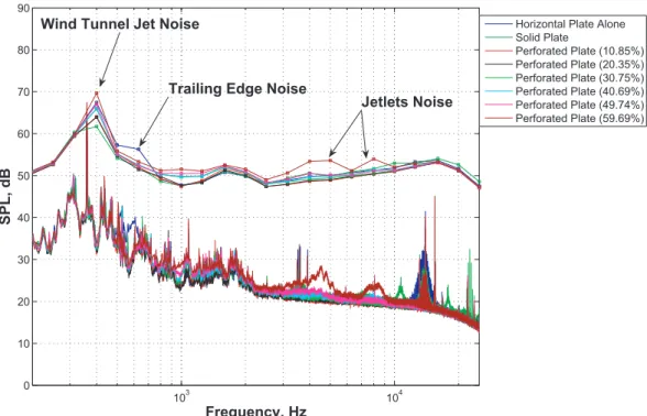
5.2 Discussion of Experimental Results . . . 109
5.2.1 Velocity Scaling . . . 114
5.3 Noise Assessment of the Perforated Plates and Configurations . . . . 118
5.4 Summary . . . 126
6 Drag Rudder Noise Assessment for SAX10 Design 129 6.1 Technical Approach . . . 129
6.1.1 Bluff-body Noise Model (Low Frequencies) . . . 129
6.1.2 Turbulent Mixing Noise Model (High Frequency) . . . 132
6.1.3 Uncertainty Analysis . . . 136
6.2 Design Implications . . . 136
6.3 Full Scale Noise Signature of Perforated Drag Rudders . . . 138
6.4 Noise Audit . . . 140
6.5 Recommendations . . . 140
7 Conclusions and Future Work 145 7.1 Conclusions . . . 145
7.2 Future Work . . . 153
A Tables 155 B Acoustic Phased Array Noise Spectra 159 B.1 Perforated Plate 1 . . . 159 B.2 Perforated Plate 2 . . . 164 B.3 Perforated Plate 3 . . . 169 B.4 Perforated Plate 4 . . . 174 B.5 Perforated Plate 5 . . . 179 B.6 Perforated Plate 6 . . . 184 C Figures 189
List of Figures
1-1 Aircraft noise sources on approach and takeoff. . . 24
1-2 Aircraft engine noise sources . . . 25
1-3 Sources of airframe noise. . . 26
1-4 Information flow in the Silent Aircraft Initiative. . . 27
1-5 Current Silent Aircraft eXperimental design SAX10. . . 28
1-6 Aircraft spoilers. . . 28
1-7 Hypothetical transformation in noise signature through perforated drag plates. . . 29
2-1 Schematic of a perforated drag plate. . . 36
2-2 Schematic of a perforated drag rudder. . . 37
2-3 Square perforated drag plate schematic with uniform perforation pattern 38 2-4 Perforated plate drag coefficient CD variation with porosity β. . . . . 42
2-5 Strouhal number versus 1/β2. . . . 43
3-1 MIT acoustic chamber and perforated drag plate test configuration. . 47
3-2 Detailed drawing of the MIT acoustic chamber. . . 48
3-3 Free-field corrections for B&K 4135 microphones with protection grid. 51 3-4 Microphone system schematic and associated hardware support. . . . 51
3-5 Sound data acquisition schematic. . . 53
3-6 Example calibration chart delivered with the condenser microphone cartridges. . . 57
3-7 Point source schematic used in facility validation. . . 63
3-9 Amount of data contamination as a function of the separation between background noise and data measurement. . . 66
3-10 Wind tunnel background noise at 150◦ directivity and 1.3 m radial
location. . . 68
4-1 Perforated plate with β = 60% porosity mounted in a spoiler configu-ration. . . 74
4-2 Detailed drawing of a perforated drag plate with β = 40% porosity. . 75
4-3 Test matrix. . . 77
4-4 Model scale noise spectra at 15 m/s. . . 78
4-5 Model scale noise spectra at 20 m/s. . . 79
4-6 Strouhal number scaling of jetlets noise of a perforated plate with 60% porosity. . . 80
4-7 Model scale noise spectra at 30 m/s. . . 81
4-8 Strouhal number scaling of jetlets noise of a perforated plate with 40% porosity. . . 82
4-9 Schematic of the MIT acoustic chamber open jet. . . 84
4-10 Schematic of the 40% perforated plate showing the row number in spoiler configuration. . . 85
4-11 SPL spectra for a 40% perforated plate at 30 m/s, rows taped from the top. . . 86
4-12 SPL spectra for a 40% perforated plate at 30 m/s, rows taped from below. . . 86
4-13 SPL normalized spectra for a 40% perforated plate at 30 m/s, rows taped from the top. . . 88
4-14 SPL normalized spectra for a 40% perforated plate at 30 m/s, rows taped from below. . . 89
5-1 Markham array system. . . 94
5-2 Markham wind tunnel background cross spectra vs 40% perforated plate spectra, scaled for L=0.3 m. . . 97
5-3 Markham wind tunnel background cross spectra vs 40% perforated
plate spectra, scaled for L=0.2 m. . . 98
5-4 Markham wind tunnel background cross spectra vs 40% perforated plate, spectra scaled for L=0.1 m. . . 98
5-5 Parameter space used in experiments. . . 100
5-6 Spoiler test configuration 1. . . 102
5-7 Phased array reference grid for spoiler test configuration 1. . . 102
5-8 Spoiler test configuration 2. . . 103
5-9 Phased array reference grid for spoiler configuration 2. . . 103
5-10 Drag rudder test configuration 1. . . 104
5-11 Phased array reference grid for drag rudder test configuration 1. . . . 104
5-12 Drag rudder test configuration 2. . . 105
5-13 Phased array reference grid for drag rudder test configuration 2. . . . 105
5-14 Noise cross spectra of small (L = 0.1 m) perforated plate 3 at 30 m/s in spoiler configuration 1. . . 109
5-15 Noise cross spectra of small (L = 0.1 m) perforated plate 5 at U∞= 30 m/s in spoiler configuration 1. . . 111
5-16 Noise cross spectra of small (L = 0.1 m) perforated plate 5 at U∞= 40 m/s in spoiler configuration 1. . . 111
5-17 Noise cross spectra of small (L = 0.1 m) perforated plate 5 at U∞= 30 m/s for the four configurations. . . 112
5-18 Velocity scaling of the peak frequencies. . . 115
5-19 Average velocity scaling of the peak frequencies. . . 116
5-20 Schematic of a perforated plate. . . 118
5-21 StL variation with plate non-dimensional parameters. . . 119
5-22 Peak A sound pressure levels as a function of the free stream velocity. 124 5-23 Peak B sound pressure levels as a function of the free stream velocity. 125 5-24 Noise cross spectra for the large perforated plate 6 at U∞ = 40 m/s for the four installation configurations. . . 126
6-1 Dipole model. . . 130
6-2 Bluff-body noise signature for ψ = 90◦ in the X −Z plane for C D(fs)=1.1.132 6-3 Low frequency bluff-body noise SPL for different ∆St. . . . 133
6-4 Drag coefficient frequency spectrum for ∆St = 0.2. . . . 133
6-5 Low frequency bluff-body noise SPL. . . 134
6-6 Measurements of SPL for a 40% perforated drag plate at free stream velocities of 15, 20 and 30 m/s. . . 135
6-7 Change in drag coefficient, ∆CD, required to balance the lift and drag over a range of approach trajectories. . . 137
6-8 Drag rudder geometry (two views). . . 137
6-9 Full scale drag rudder noise scaled from measurements and dipole model.139 6-10 Perforated drag rudder noise hemispheres . . . 141
6-11 Overview of propagation effects. . . 142
B-1 Perforated plate 1 used in drag rudder configuration 1. . . 159
B-2 Perforated plate 1 with L = 0.1 m in spoiler configuration 1. . . . 160
B-3 Perforated plate 1 with L = 0.2 m in spoiler configuration 1. . . . 160
B-4 Perforated plate 1 with L = 0.1 m in spoiler configuration 2. . . . 161
B-5 Perforated plate 1 with L = 0.2 m in spoiler configuration 2. . . . 161
B-6 Perforated plate 1 with L = 0.1 m in drag rudder configuration 1. . . 162
B-7 Perforated plate 1 with L = 0.2 m in drag rudder configuration 1. . . 162
B-8 Perforated plate 1 with L = 0.1 m in drag rudder configuration 2. . . 163
B-9 Perforated plate 1 with L = 0.2 m in drag rudder configuration 2. . . 163
B-10 Perforated plate 2 used in drag rudder configuration 1. . . 164
B-11 Perforated plate 2 with L = 0.1 m in spoiler configuration 1. . . . 165
B-12 Perforated plate 2 with L = 0.2 m in spoiler configuration 1. . . . 165
B-13 Perforated plate 2 with L = 0.1 m in spoiler configuration 2. . . . 166
B-14 Perforated plate 2 with L = 0.2 m in spoiler configuration 2. . . . 166
B-15 Perforated plate 2 with L = 0.1 m in drag rudder configuration 1. . . 167
B-17 Perforated plate 2 with L = 0.1 m in drag rudder configuration 2. . . 168
B-18 Perforated plate 2 with L = 0.2 m in drag rudder configuration 2. . . 168
B-19 Perforated plate 3 used in drag rudder configuration 1. . . 169
B-20 Perforated plate 3 with L = 0.1 m in spoiler configuration 1. . . . 170
B-21 Perforated plate 3 with L = 0.2 m in spoiler configuration 1. . . . 170
B-22 Perforated plate 3 with L = 0.1 m in spoiler configuration 2. . . . 171
B-23 Perforated plate 3 with L = 0.2 m in spoiler configuration 2. . . . 171
B-24 Perforated plate 3 with L = 0.1 m in drag rudder configuration 1. . . 172
B-25 Perforated plate 3 with L = 0.2 m in drag rudder configuration 1. . . 172
B-26 Perforated plate 3 with L = 0.1 m in drag rudder configuration 2. . . 173
B-27 Perforated plate 3 with L = 0.2 m in drag rudder configuration 2. . . 173
B-28 Perforated plate 4 used in drag rudder configuration 1. . . 174
B-29 Perforated plate 4 with L = 0.1 m in spoiler configuration 1. . . . 175
B-30 Perforated plate 4 with L = 0.2 m in spoiler configuration 1. . . . 175
B-31 Perforated plate 4 with L = 0.1 m in spoiler configuration 2. . . . 176
B-32 Perforated plate 4 with L = 0.2 m in spoiler configuration 2. . . . 176
B-33 Perforated plate 4 with L = 0.1 m in drag rudder configuration 1. . . 177
B-34 Perforated plate 4 with L = 0.2 m in drag rudder configuration 1. . . 177
B-35 Perforated plate 4 with L = 0.1 m in drag rudder configuration 2. . . 178
B-36 Perforated plate 4 with L = 0.2 m in drag rudder configuration 2. . . 178
B-37 Perforated plate 5 used in drag rudder configuration 1. . . 179
B-38 Perforated plate 5 with L = 0.1 m in spoiler configuration 1. . . . 180
B-39 Perforated plate 5 with L = 0.2 m in spoiler configuration 1. . . . 180
B-40 Perforated plate 5 with L = 0.1 m in spoiler configuration 2. . . . 181
B-41 Perforated plate 5 with L = 0.2 m in spoiler configuration 2. . . . 181
B-42 Perforated plate 5 with L = 0.1 m in drag rudder configuration 1. . . 182
B-43 Perforated plate 5 with L = 0.2 m in drag rudder configuration 1. . . 182
B-44 Perforated plate 5 with L = 0.1 m in drag rudder configuration 2. . . 183
B-45 Perforated plate 5 with L = 0.2 m in drag rudder configuration 2. . . 183
B-47 Perforated plate 6 with L = 0.1 m in spoiler configuration 1. . . . 185
B-48 Perforated plate 6 with L = 0.2 m in spoiler configuration 1. . . . 185
B-49 Perforated plate 6 with L = 0.1 m in spoiler configuration 2. . . . 186
B-50 Perforated plate 6 with L = 0.2 m in spoiler configuration 2. . . . 186
B-51 Perforated plate 6 with L = 0.1 m in drag rudder configuration 1. . . 187
B-52 Perforated plate 6 with L = 0.2 m in drag rudder configuration 1. . . 187
B-53 Perforated plate 6 with L = 0.1 m in drag rudder configuration 2. . . 188
B-54 Perforated plate 6 with L = 0.2 m in drag rudder configuration 2. . . 188
C-1 St(s−d) variation with plate non-dimensional parameters . . . 190
C-2 Std variation with plate non-dimensional parameters . . . 191
C-3 Sts variation with plate non-dimensional parameters . . . 192
List of Tables
3.1 Microphone position. . . 49
3.2 Summary of the key specifications for B&K 4135 microphones. . . 50
3.3 Channel, DAQ rate, and resolution specifications for a NI PCI-6143 DAQ card . . . 52
3.4 Time domain characteristics of rectangular and Hanning weighting functions. . . 55
3.5 Frequency domain characteristics of rectangular and Hanning weight-ing functions. . . 55
3.6 Summary of B&K 4135 microphone calibration coefficients, both fac-tory and measured. . . 60
4.1 Characteristics of the test plates. . . 75
4.2 Expected SPL reduction if a specified number of rows are taped com-pared to the case when no rows are taped for the 40% porous plate. . 87
5.1 Design characteristics of the perforated plates. . . 101
5.2 Porosity, drag coefficient and Strouhal number of the tested perforated drag plates. . . 120
5.3 Area increase factors for the tested perforated plates. . . 120
5.4 OASPL corrected for drag. . . 122
5.5 Calculated speed dependance n of plate noise levels for perforated plate 6. . . 123
A.2 Peak magnitudes for small plates (L = 0.1 m) in spoiler configuration 1.156
A.3 Peak frequencies for large plates (L = 0.2 m) in spoiler configuration 1. 156
Chapter 1
Introduction
Historically, noise is one of the principal environmental issues for aviation. Aircraft noise is particularly annoying to people living in areas around airports despite con-siderable reductions in noise and a corresponding decrease in the population around airports. Air traffic keeps increasing as does pressure from the public to control the increase in aircraft noise. Moreover, concern about noise remains a constraint on efforts to expand airport capacity to meet the growing demand for air travel.
One region in which aircraft noise has been extensively studied and controlled is the United Kingdom. Estimates from the United Kingdom Department for Trans-portation put noise costs for London Heathrow airport in the range of £293 million (approximately $571 million) in lost property value alone [1].
One way to solve this problem is to introduce quieter aircraft. Research at MIT and Cambridge University was initiated to design a Silent Aircraft1. The transition to quieter aircraft is expected to benefit communities, airports, and airlines. The levels of noise affecting communities near airports are expected to decline, providing a better quality of life for those communities. That decline is, in turn, expected to reduce community opposition to airport operations and expansion and to reduce the demand for funds provided for noise abatement through federal grants and user charges. The airlines expect the transition to facilitate their long-term planning for
1Silent means sufficiently quiet that outside the airport perimeter aircraft noise is less than the
Figure 1-1: Aircraft noise sources on approach and takeoff [3].
investment and fleet operations. These expectations vary concerning the extent to which the airlines would replace rather than convert old aircraft to comply with the new noise requirements [2].
1.1
Background
1.1.1
Aircraft Noise Sources
The noise generated by a transport aircraft can be divided in two main groups: one due to airframe and other due to engine noise sources. The absolute and relative levels of each of the noise sources depend on the aircraft configuration. The various noise sources on a conventional transport aircraft are shown in Figure 1-1 for the takeoff and approach configurations.
Engine noise sources include fan and compressor noise, turbine noise, combustion (core) noise and jet noise (see Figure 1-2). In the past, turbojet engines were the dominant noise source both on approach and takeoff. Since the introduction of
high-Figure 1-2: Aircraft engine noise sources
bypass turbofan engines and acoustic liners, the engine noise was significantly reduced (by of over 10 EPNdB [4]). Currently, acoustic liners are used in the inlet, fan case, aft bypass duct, and core nozzle to attenuate both fan and core engine noise. These passive liners are tuned to be most effective at frequencies in the peak annoyance range (2-4 kHz).
The airframe is an important noise source from a large aircraft in its landing configuration as the level of noise may only be a few decibels below the level of noise radiated from the engines. The airframe noise is due to unsteady flow from wing and tail trailing edges, turbulent flow through and around deflected wing trailing edge flaps and leading edge slats, flow past landing gear shafts, and other undercarriage elements, fuselage and wing turbulent boundary layers, panel vibrations, and high-speed airflow past contours and cavities such as uncovered wheel wells (see Figure 1-3).
Much research is aimed at reducing airframe noise contribution by improving the ‘smoothness’ of the flow over the most critical components. The longer-term solution of this problem is a Silent Aircraft that can operate within this air transportation system.
Figure 1-3: Sources of airframe noise (picture courtesy of Ben Pritchard, Airlin-ers.net).
1.1.2
Silent Aircraft Initiative
Within this context, the Silent Aircraft Initiative (SAI) funded by the Cambridge-MIT Institute (CMI) was launched. The objective of the SAI is to achieve a step-change in noise levels compared to current practice and this will require a radically different approach to the problem. This is a multidisciplinary problem involving airframe, engine, and operation design teams. Assessment of the economic impact of a Silent Aircraft is also under investigation. The design process of such an aircraft requires close interaction between the design teams. The information flow is shown in Figure 1-4.
This information flow establishes the framework for a fully integrated and opti-mized for noise Silent Aircraft. The boxes represent the different research areas. In each of these areas, the aim is to use both analytical techniques and experimental measurements to assess potential solutions and to validate advanced prediction tools, which will then be used to scale the results to a full size aircraft.
In order to reduce airframe and propulsion system noise levels below the back-ground noise in well-populated areas, noise must be a prime design variable. It is also clear that conceptually new aircraft configurations should be studied. A
blended-Figure 1-4: Information flow in the Silent Aircraft Initiative [5].
wing-body type aircraft configuration with aerodynamically-smooth lifting surfaces is a potential candidate to achieve the airframe noise reduction goals. The current Silent Aircraft eXperimental design, SAX10, is shown in Figure 1-5.
However, mitigating airframe noise emissions by removing the high-lift devices (leading edge slats and trailing edge flaps) invariably leads to a reduction in the drag. Also, when using a steeper approach profile, during which the noise sources are further from the ground and the noise levels are lower because of the atmospheric and geometric attenuation, a lot of drag need to be generated. Thus, one of the most critical tasks in noise reduction is to develop technologies to increase drag in quiet ways.
One way to dissipate the energy on approach is to use deployable low-noise high-drag structures. Conventional spoilers as those shown in Figure 1-6 create high-drag in a noisy manner. The processes that lead to drag on such bluff bodies involve unsteady wakes and inevitably generate noise.
So far, relatively little analysis has been done to investigate the possibility of gener-ating drag quietly during approach. Noise reduction should be considered along with the performance (drag generation) penalty. Therefore, silent drag concepts should be investigated to determine how much drag could be produced with satisfactory noise
(a) Top section view [5]. (b) Design rendering (picture courtesy of Steve Thomas).
Figure 1-5: Current Silent Aircraft eXperimental design SAX10.
Low Frequency Noise (Large Length Scales)
SPL, dB
Frequency, Hz
High Frequency (Small Length Scales)
Figure 1-7: Hypothetical transformation in noise signature through perforated drag plates.
reduction.
1.2
The Idea Behind Silent Spoiler/Drag Rudder
The idea behind a silent spoiler/drag rudder is to alter the noise production mecha-nism by perforating the spoilers/drag rudders. It is hypothesized that, by introducing perforations the large length scales responsible for the noise radiated by unsteady vortical structures are changed to small length scales driving jet noise, which at high frequencies are attenuated more effectively and perceived less annoying to the human ear. This transformation of the noise signature is depicted in Figure 1-7.
Jet and jet noise studies [6, 7] also suggest that the peak frequency associated with mini-jets is shifted to higher frequencies and that the mini-jets interfere to pro-duce a lower sound pressure level. Atmospheric attenuation, on the other hand, increases nearly exponentially with increasing frequency, and spectral noise compo-nents contribute less to the Effective Perceived Noise Level (EPNL)2 noise metric
2This is a metric used to describe the tone-sensing characteristic of the human hearing system
as the frequency increases above 4 kHz. Humans have a low sensitivity to acoustic frequencies above 10 kHz and noise at frequencies higher than 10 kHz is not included in the calculation of EPNL. This idea may be applied to the noise produced by a perforated plate resembling an array of low speed mini-jets. The perforated spoil-ers/drag rudders could help reduce noise produced by current and future generations of aircraft.
One of the main challenges of designing quieter drag devices is that current an-alytical models do not accurately predict the noise that would be emitted by such designs. Also, the effect that such designs may have on the lift and drag of the wing has not been investigated. Therefore, it is necessary for an actual model to be built and tested to determine the potential noise reduction that can be achieved by using such silent drag devices.
The work presented in this thesis focuses primarily on aeroacoustic tests and analysis of perforated drag plates.
1.2.1
Research Objectives
The primary objective of these aeroacoustic experiments is to asses the acoustic ben-efits and impact on drag of a perforated spoiler/drag rudder. The second objective is to assess the strength and if possible, determine the directivity of the noise sources (bluff-body and turbulence mixing noise) of such perforated plates. The third ob-jective is to assess different configurations of perforated drag devices. The fourth objective is to find scaling laws for the perforated plate noise spectra. These scaling laws are envisioned to help establish a prediction model for the acoustic signature of perforated drag devices to be used on a Silent Aircraft.
1.2.2
Research Questions
The main research question is to determine for a fixed level of drag what noise reduc-tion potential can be achieved by perforating the drag plates.
1.2.3
Success Goals
The primary success goal is to demonstrate a net benefit in the acoustic signature of perforated drag plates compared to a solid plate on the same drag basis.
The second success goal is to show that low frequency noise is reduced and that the turbulence mixing noise generated at mid frequencies is shifted to higher frequencies.
1.2.4
Technical Approach
To meet the research objectives, first the noise mechanisms associated with perforated drag plates are identified together with the non-dimensional parameters governing these noise mechanisms. Second, a drag analysis is conducted to investigate the effect that perforations have on the drag generation of such perforated plates.
Conducting aeroacoustic tests using advanced equipment such as an acoustic phased array is expensive and requires careful planning. Thus, fast and most im-portantly inexpensive aeroacoustic tests are needed to get preliminary results of the noise characteristics of perforated drag plates.
A preliminary test campaign is conducted in the acoustic chamber facility at the Massachusetts Institute of Technology (MIT). First, the chamber is acoustically characterized. Then, aeroacoustic tests of perforated plates are conducted. The data is analyzed and the results are used for development of a preliminary noise prediction tool.
Based on the preliminary acoustic test campaign at MIT, the parameter space of perforated drag plates is defined and later explored in the Markham wind tunnel at Cambridge University (CU). The Markham wind tunnel is equipped with an acoustic phased array which provides a powerful measurement capability that can identify noise 15 dB below the wind tunnel background noise [9].
1.3
Thesis Outline
Chapter 2 presents the noise mechanisms and dimensional analysis of the key geo-metric and fluid dynamic parameters that govern the noise generation of a perforated drag plate. A drag analysis to investigate the effects of the perforations on the drag generation is then discussed.
In Chapter 3, a characterization of the acoustic chamber at MIT is presented together with the test equipment calibration procedure and data reduction technique. Chapter 4 presents a combined experimental and analytical effort that was con-ducted to determine the noise signature of perforated drag plates.
In Chapter 5, the parameter space of perforated drag plates is first defined and then explored through a series of aeroacoustic tests conducted in the Markham wind tunnel at Cambridge University. The results and data analysis are discussed.
In Chapter 6, a prediction tool for a perforated drag rudder configuration is de-veloped on the basis of the MIT acoustic chamber experimental results.
Chapter 2
Description of Noise and Drag
Mechanisms of Perforated Drag
Plates
This chapter presents the noise mechanisms and dimensional analysis of the impor-tant geometric and fluid dynamic parameters that govern the noise generation of a perforated drag plate. A drag analysis to investigate the effects of the perforations on the drag generation is also discussed.
2.1
Noise Mechanisms Associated with Perforated
Drag Plates
The true sources of aerodynamic noise are the fluid disturbances themselves. The interaction of these disturbances with airframe structural discontinuities causes sub-stantial sound radiation. It is believed that there are three major noise source mech-anisms associated with perforated drag plates:
• Bluff-body noise due to the flow separation at the side edge. The unsteady motions in the shear layer are a major noise source.
• Turbulence mixing noise by the individual jetlets that comprise the perfo-rated drag plate and their interaction with the bluff-body wake.
• Panel vibration noise due to the mechanical vibration of the plate.
The difficulty is that these noise mechanisms are interacting with one another. This makes their individual identification very complicated. On the other hand the strong coupling is the reason why a noise reduction could be achieved (see Section 1.2).
Characteristics of the individual mini-jet nozzles that comprise the perforated drag plate are jet-to-jet shielding and coalescence into a larger jet. This is a critical factor in order to realize acoustic suppression from any distribution of the perforations. Without enough separation of the mini-jets, they will coalesce into a larger jet with a noise signature more characteristic of a single larger jet rather than many small jets. Different designs of perforations will have different effect on the perforated drag plate noise signature. Having perforations closer to the drag plate edges will relieve the pressure distribution and this affects the vortex shedding from the edge. Thus, in order to fully understand the noise generation of a perforated drag plate different perforation patterns need to be tested. The relation of the separation and the per-forations’ diameter that gives satisfactory acoustic suppression without considerable drag penalty is what needs to be found.
Another significant noise mechanism of the perforated drag plate is associated with panel vibration driven by turbulent pressure fluctuations. Dowell [10] has given a simple estimate of the far-field radiation from the lowest order mode of a rectan-gular panel under turbulent excitations. For a panel of area 3 ft2, he found a lowest eigenfrequency of 37 Hz and a sound pressure level (SPL) of 97 dB at a range of 300 ft. This estimate is very sensitive to the modeling of the surface pressure field, which may itself be significantly changed by the vibration, especially if the dominant radia-tion is from a high order panel mode. The principal sites of vibraradia-tion are likely to be associated with regions in which the surface pressure modeling is probably inaccurate. Thus, the theoretical work seems of little help in those circumstances [11]. Panel
vi-bration noise is also difficult to be tested as the vivi-brations depend not only on the perforated drag plate design but also on the way it is secured to the wing or winglet. Thus, the current study does not focus on this noise mechanism but considers it as a possible and significant noise source.
The interaction of flow with structure, or sound generated by fluid flow is in the class of wake flows, which occur in the separated flow behind the drag plate. The wakes, highly coherent or very random, produce fluctuating forces on the element “shedding” the wake in both the streamwise (drag) and normal-to-streamwise (lift) direction. These force fluctuations may be characterized as acoustic dipoles, whose far-field sound exhibits a known dependence on frequency, amplitude, and direction (which may be determined from flow speed and element geometry). The strength of the bluff-body effects depends not only on the flight conditions such as angle of attack and flight speed but also on the spoiler/drag rudder location because of the interaction with local flow. The noise signature of the bluff-body effect could be modeled by an array of independent acoustic point dipoles along the surface of the plate.
As mentioned before, the main challenge is that these noise mechanisms are inter-acting with one another which makes their individual identification very complicated. This complication is reduced then by a dimensional analysis identifying the important non-dimensional groups that govern these noise mechanisms.
2.2
Dimensional Analysis
The optimal perforated drag plate is one that achieves a balance of reducing the noise without sacrificing the drag generating ability of the plate. In order to find the optimal design the critical parameters that describe the noise mechanisms associated with a perforated plate need to be determined.
Dimensional analysis offers a method for reducing complex physical phenomena to a simple form prior to obtaining a qualitative answer. The premise of this type of analysis is that the form of any physically significant equation must be such that the
Figure 2-1: Schematic of a perforated drag plate.
relationship between the actual physical quantities remains valid independent of the magnitudes of the base units [12].
A simple non-dimensional model can provide a parametric guideline for sizing the perforated drag plates to be tested and helps predict and scale some important features of the flow and the noise generation mechanisms.
An enlarged view of a perforated drag plate is shown in Figure 2-1. In this model, the horizontal separation defined as the horizontal distance between two neighboring perforations is denoted by x. The vertical separation is denoted by y. The porosity of such a plate, defined as the ratio of the open to total area, can be calculated using the following equation
β = πd
2
4xy. (2.1)
The parameters that are sufficient to define the flow and geometry of the perforated drag plates are: the free stream velocity U∞in m/s, the speed of sound a∞in m/s, the
air density ρ∞in kg/m3, the air viscosity µ in kg/ms, the diameter of the perforations
d in m, the horizontal separation x in m, the vertical separation y in m, the frequency f in Hz, the deployment angle ψ in deg, the plate height H in m, the plate length L in m, the distance to an observer r in m, and directivity angle θ in deg. The deployment angle ψ is defined as the angle between the winglet axis and the drag plate axis. Figure 2-2 shows a conceptual design of perforated drag rudder used on
Figure 2-2: Schematic of a perforated drag rudder.
the current Silent Aircraft design.
The Buckingham π-theorem can be used to express any physical quantity of inter-est such as the sound pressure level, as a function of the non-dimensional quantities
SP L = f µ x L, y L, f L U∞ ,ρ∞LU∞ µ , U∞ a∞ , d L, H L, ψ, θ, r L ¶ . (2.2)
The third argument in Equation 2.2 is the Strouhal number
StL=
f L
U∞
, (2.3)
while the fourth non-dimensional group is the Reynolds number based on the length L of the perforated drag plate
ReL =
ρ∞LU∞
µ . (2.4)
The equation for the porosity, β, expressed using the non-dimensional parameters is as follows β = π 4 µ d L ¶2µ x L ¶−1µ y L ¶−1 . (2.5)
Figure 2-3: Square perforated drag plate schematic with uniform perforation pattern
2-3), Equations 2.2 and 2.5 simplify to the following SP L = f µ s L, StL, ReL, M, d L, ψ, θ, r L ¶ , (2.6) β = π 4 µ d L ¶2µ s L ¶−2 . (2.7)
An L × L perforated square plate with a uniform perforation pattern consists of N small s × s squares plates (Figure 2-3). Therefore,
s
L =
r 1
N. (2.8)
Thus, s/L in Equation 2.6 takes only discrete values. The exact forms of (2.2) and (2.6) can be discovered by experimentation or by solving the problem theoretically. The forms obtained so far reduce the number of variables and simplify the analysis of the situation.
2.3
Drag Analysis
It is misleading to only consider noise suppression without considering the associated performance penalty of perforated drag plates. Thus, noise assessment of potential
perforated drag devices should always be made on the same drag basis. For this purpose, a drag analysis is conducted to investigate the effect of perforations on the drag generation of such perforated plates. For the current study, it was hypothesized that the plate drag coefficient depends only on the plate porosity and an analytical expression exists that captures this variation. This hypothesis was based on the Tay-lor’s theory [13]. Considering the perforated plate to be an assemblage of uniformly spaced centers of resistance, Taylor found that
CD =
κ (1 + 1
4κ2)2
. (2.9)
Here κ is expressed in terms of the pressure drop across the plate such that p1− p2 = κ µ 1 2ρu 2 ¶ , (2.10)
where p1 is the static pressure on the upstream side, p2 that on the downstream side of the plate, u the mean air velocity through it, and κ the plate resistance to a passage of air. Since the flow through the perforated plate can take place only in the holes, the resistance κ of the plate depends on its porosity. However, Equation 2.9 for the drag coefficient suggests that CD cannot be greater than 1.0. This is not true
as the drag coefficient of a high-resistance plate must approach that of a solid plate placed perpendicular to the air flow. The drag coefficient for such a bluff body was experimentally determined by Castro [14] and found to be 1.89. Taylor [13] suggests that this discrepancy may be due to the fact that the mixing of the wake with the air which has not passed through the perforated plate can increase the negative pressure at the back of the screen, and this is not modeled in his theory.
On the other hand, Eckert and Pfluger [15] found that the resistance κ takes the form κ = µ 1 − β β ¶2 , (2.11)
the resistance κ with porosity
κ + 1 = 1 − γ
β2C2. (2.12)
Here C is the contraction coefficient for a fluid flowing through a perforation, while γ is the fraction of the lost pressure which is regained when the stream again becomes uniform behind the plate,
p2 − pc = 1 2γρ µ u βC ¶2 , (2.13)
where pc is the pressure in the contraction.
Equation 2.12 is consistent with Equation 2.11 since both C and γ may depend on β. Then, substituting Equation 2.11 or 2.12 in Equation 2.9, the drag coefficient can be expressed as a function of β only.
Davies [16] carried out measurements of the air resistance of perforated plates and gauzes to test this theory and to explore the connection between the resistance κ and the porosity β. He found that the data do not collapse based on Equation 2.11 given by Eckert and Pfluger. The discrepancy suggests that the jets do not recover a constant portion of their kinetic energy as it was assumed deriving Equation 2.11. He also found that for perforated plates there is a steady and slow increase in (κ + 1)β2 as β decreases.
Although, the variation of the resistance κ with β cannot be exactly derived and experimental data is usually used to get this variation, Taylor’s theory was proved valid for κ < 4 or plates with high porosity. This suggests that there might be two regimes for the flow behind the perforated plate, one for low porosity plates and one for high porosity plates.
It is obvious that a more thorough understanding of the flow behind a perforated plate is needed in order to find the drag coefficient variation with plate porosity.
Next the physics of flow behind a perforated plate is considered. A bluff body usually sheds two shear layers which are unstable and interact in the near wake, rolling up to form a vortex street. If the two separating shear layers are prevented from interacting in the usual way, as is the case with a splitter plate, the vortex formation may be delayed and the vortex formation point moves downstream. When
the plate is perforated extra air is injected between the two shear layers and they do not meet but sill interact.
At low values of porosity the two shear layers are not prevented from interacting and they form a vortex street that will dominate the wake. As the porosity increases, more bleed air is introduced, the vorticity in the shear layers decreases. There is also a corresponding increase of base pressure and hence a decrease in drag. Thus, the vortex street strength gradually decreases when the porosity increases. This also reduces the noise levels at low frequencies that are mainly due to the vortices shed by the plate.
As the plate porosity increases, the extra air injected increases and if enough air is injected between the two shear layers, they could be prevented from interacting at all. To conserve the mass balance across the wake there still has to be a reversed flow region, and this moves downstream with increasing porosity β.
It was hypothesized that if the porosity is high enough the flow will change its characteristics from flow dominated by the vortex street to flow dominated by the turbulence or from large length scale structures dominated to small length scale struc-tures dominated.
This change of the flow regimes was observed by Castro [14]. He investigated the flow in the wakes behind two-dimensional perforated plates. Measurements of drag and shedding frequency were made in the Reynolds number range 2.5 × 10⁴ < Re < 9.0 × 10⁴.
The drag coefficient was defined as
CD =
Drag F orce 1
2ρU∞2 A
, (2.14)
where A is the plate area.
Figure 2-4 shows a plot of the drag coefficient, CD, as a function of 1/β2 obtained
by both wake traverses and drag balance methods at Re = 9 × 10⁴. The expression 1/β2 was used as the ordinate since it is a relevant parameter in Taylor’s theory.
Figure 2-4: Perforated plate drag coefficient CD variation with porosity β (Castro[14]), − · −, Blockley[17], − ◦ −, wake traverse method, −2−, drag balance method.
predictions by Taylor and at lower values (high 1/β2) the agreement is not so good. By placing a hot wire outside the wake to obtain a frequency shedding signal Cas-tro [14] also measured the vortex shedding frequency. Figure 2-5 shows the SCas-trouhal number, defined as St = f L/U∞, where f is the shedding frequency, L the plate
chord and U∞ the free stream speed, again plotted against 1/β2. The Strouhal
num-ber was measured over a range of Reynolds numnum-ber, but only the two sets of results corresponding to the two limits of the range are shown. As β increases there is a gradual increase in Strouhal number until at β = 0.2, where an abrupt reversal of slope is present. However, there is still a distinct peak in the spectrum, and only when β exceeds about 0.4 does this peak begin to spread over a range of values. At this stage it is no longer possible to pinpoint any dominant frequency [14]. Therefore, Figure 2-5 shows a band of possible values of St at these high values of porosity.
It was observed by Castro [14] that at β of about 0.2 there are quite abrupt changes in the drag coefficient and Strouhal number. Figure 2-4 shows a sudden drop in the drag coefficient. If the vortex street died gradually a smooth continuation of
Figure 2-5: Strouhal number versus 1/β2 (Castro[14]), − ◦ −, Re = 2.5 × 10⁴,− × −,
Re = 9 × 10⁴.
the drag coefficient curve at high values of β into the low β range should be present. The drag of a body shedding a vortex street is substantially higher than if the vortex street is not present, so Figure 2-4 suggests that at β of 0.2 the vortex street suddenly ceases to exist. There is a corresponding drop in the Strouhal number as Figure 2-5 suggests. Castro argues that this is a critical point, at which there is just enough bleed air to prevent the shear layer from interacting at all to form a vortex street. If this is the case, a ‘shedding frequency’ or ‘Strouhal number’ can not be defined in the same sense beyond this critical value of β, but he still found a dominant frequency probably connected with the jetlets or some sort of far wake instability.
The abrupt changes in CD and St, observed by Castro [14], proved that there
indeed exist two flow regimes behind the perforated plate, one at low porosity and the other at high porosity of the plate. The critical value of β seems to be of about 0.2. In the first flow regime, appropriate to low values of porosity, the vortex street (large length scales) dominates the wake. In the second flow regime, at high values of porosity the small length scales dominate the wake. Because a proper analytical expression for the drag coefficient was not found, data obtained by Castro [14] is used to obtain the drag coefficient for a given perforated plate in this study.
Chapter 3
MIT Acoustic Chamber Design
and Instrumentation
One of the main challenges of designing quieter drag devices is that current analytical models do not accurately predict the noise that is emitted by such designs. Therefore, it is necessary to build an actual model and test it to determine any noise reduction that can be achieved by using perforated drag plates.
Conducting aeroacoustic tests in Markham wind tunnel at Cambridge University, equipped with a phased microphone array is expensive and requires careful planning. The test articles should be sized properly to yield noise spectra above that of the wind tunnel background noise and within the desired frequency range. Thus, low cost acoustic tests were first conducted at MIT to get preliminary results of the noise characteristics associated with perforated drag plates.
Aeroacoustic tests of perforated plates mounted on a horizontal plate in a spoiler configuration were conducted in the MIT acoustic chamber placed in front of the 1-by-1 Foot Low-Speed Wind Tunnel. These preliminary results were then used to derive the first scaling laws and to size the test articles for the detailed aeroacoustic tests in the Markham wind tunnel.
The main purpose of the MIT acoustic chamber is to minimize the effect of ambient noise on test article noise measurements driven the 1-by-1 Foot Low-Speed Wind Tunnel. The chamber is located inside the Gerhard Neumann Hangar and Laboratory
at MIT. This chapter introduces the design of the MIT acoustic chamber, microphone and associated support instrumentation, measurement technique and characterization of the MIT acoustic chamber.
3.1
Acoustic Facility Design
The goal in source characterization is to determine quantities that are independent of the particular acoustical environment or installation. This permits the prediction of characteristics in other environments or installations.
Reflections and reverberations from surrounding objects produce standing waves at the point of observation. Such distortions are caused by interaction between the directly incident wave and the returning reflections. In order to make measurements in a free-field, without reflecting objects, the measurements must be made outdoors at the top of a flagpole or in an anechoic chamber.
Originally, the MIT acoustic chamber was constructed for an undergraduate project [18]. The ceiling, floor and all the walls of the chamber are covered with acoustic foam forming wedges of ∼5 cm size such that the small reflections with the wall are di-rected again and again into the absorbent material until essentially all the energy is absorbed. In such an anechoic environment, sound simply travels outward and away from the source, with no return and without the presence of interfering reflections.
Figure 3-1 shows the inside of the acoustic chamber with a perforated drag plate test configuration. A more detailed drawing is presented in Figure 3-2. The duct inside the acoustic chamber attaches to the MIT 1-by-1 Foot Low-Speed Wind Tunnel. With the help of brackets and adhesive sealant between them air is prevented from bleeding. There is a rectangular opening at the wall opposite the duct through which the wind tunnel jet exhausts to the outside. Figure 3-2 also shows four thin aluminum arcs on which 12 microphones are mounted. The microphone assembly is discussed next.
Figure 3-2: Detailed drawing of the MIT acoustic chamber. Red dots indicate micro-phone locations.
3.1.1
Microphone Placement
An important characteristic in aeroacoustics is source directivity because what might be perceived as a noise reduction at one location could be a shift in acoustic energy from one direction to another. Ideally, a map of the sound field on a sphere surround-ing the noise source is desired. However, when there is symmetry in the noise field, as is the case for the perforated spoiler tests performed in this study, the microphones can be distributed on a one-eighth sphere.
The microphone array (see Figure 3-2) in the MIT acoustic chamber was arranged to create an eight-sphere with radius 1.5 m. The center of the sphere is the wind tunnel duct exit. The entire aluminum microphone mount was attached directly to the roof of the acoustic chamber. The twelve microphones and their azimuthal and elevation position are tabulated in Table 3.1. Throughout this thesis the microphone locations are referred to by their angle of azimuth and elevation.
Next, the acoustic instrumentation used in the preliminary aeroacoustic tests is discussed.
Table 3.1: Microphone position. Microphone Microphone Number Location 1 (0◦, 75◦) 2 (0◦, 60◦) 3 (0◦, 45◦) 4 (30◦, 75◦) 5 (30◦, 60◦) 6 (30◦, 45◦) 7 (60◦, 75◦) 8 (60◦, 60◦) 9 (60◦, 45◦) 10 (90◦, 75◦) 11 (90◦, 60◦) 12 (90◦, 45◦)
3.2
Acoustic Instrumentation
This section outlines the microphones used, the calibration procedures and the asso-ciated data acquisition system.
3.2.1
Microphone Instrumentation
All acoustic measurements at MIT were conducted using Br¨uel & Kjær (B&K) 4135, 1/4 inch free-field microphones, which are able to measure the sound pressure levels over a frequency of 4 Hz through 100,000 Hz. Table 3.2 summarizes some of the key properties for this type of microphone.
The B&K 4135 is a condenser type microphone. The small 1/4” diameter pro-vides higher limits for the frequency and dynamic ranges, at the expense of a lower sensitivity. B&K 4135 has very high relative impedance and linearity. Some of the advantages of this type of microphone are the stability (holds calibration), low sensi-tivity to vibration and the wide range.
B&K 4135 microphones are sensitive to temperature and pressure variations, rela-tively fragile and require high polarizing voltage and impedance-coupling device near the microphone. These microphones obtain the charge for the electric field from a
Table 3.2: Summary of the key specifications for B&K 4135 microphones [19].
Microphone Property Description / Value
Frequency Response Characteristic Free-field 0◦ Incidence
and Random Incidence Open Circuit Frequency Responsea (2dB) 4 Hz to 100 kHz
Open Circuit Sensitivity 4 mV/Pa
Lower Limiting Frequency (-3 dB) 0.3 Hz to 3 Hz
Cartridge Thermal Noise 29.5 dB
Resonance Frequencyb 100 kHz
Polarization Voltage 200 V
aNot for random incidence.
b90◦ phase shift of pressure characteristic.
DC power supply connected to the microphone via the preamplifier [19]. This DC power is provided by the Microphone Multiplexer Type 2822. Due to the high charge resistance of the preamplifier, the charge build-up on the backplate is not instanta-neous. Thus, the externally polarized B&K 4135 microphone only reaches the correct working voltage after about one minute. Before this time a microphone may not be within specification.
When using a B&K 4135 microphone, the microphone should be pointed towards the source. Figure 3-3 shows the free-field corrections for a B&K 4135 microphone with incidence angle. For the conducted experiments, the microphones were oriented at zero incidence angle to the source/test article and grid caps were left on to protect the microphone.
The microphones are connected to a 1/2 inch B&K 4135 preamplifier Type 2669 using a UA 0035 1/4 to 1/2 inch adapter. The preamplifier has a very high input impedance presenting virtually no load to the microphone [20]. The high output volt-age together with a low inherent noise level gives a wide dynamic range. The frequency response of the preamplifier is ±0.5 dB between 3 Hz to 200 kHz. The preamplifiers are then connected to a 2669 B cable, which in turn connects to B&K Microphone Multiplexer 2822. A schematic of the microphone assembly and associated hardware support is shown in Figure 3-4. A BNC cable connects the Multiplexer 2822 with the data acquisition system (DAQ) used for the acoustic experiments conducted at MIT.
Figure 3-3: Free-field corrections for B&K 4135 microphones with protection grid [19].
Table 3.3: Channel, speed, and resolution specifications for a NI PCI-6143 DAQ card [21]
PCI-6143 DAQ Property Description / Value
Bus PCI, PXI
Analog Inputs 8
Input Resolution 16 bits
Sampling Rate 250 kS/s per channel
Input Range ±5 V
Digital I/O 8
Counter/Timers two 24-bit
Trigger Digital
3.2.2
Data Acquisition System
The output signal from the multiplexer through a BNC cable is fed into a National Instruments BNC-2110 shielded connector block. A SHC68-68-EP Noise-Rejecting, Shielded Cable connects the NI BNC-2110 to the NI PCI-6143 DAQ card. The NI PCI-6143 is a high-speed continuous data logging (speeds of 2 MS/s aggregate per board) card that has high dynamic accuracy and simultaneity. Table 3.3 summarizes the specification details of a NI PCI-6143 DAQ card.
Figure 3-5 shows the block diagram describing how the sound data was actually acquired. As depicted, the signal from the microphone is first transmitted through a preamplifier and a multiplexer. The multiplexer acts as an interface to the DAQ board. The DAQ board converts the signal into a digital format and feeds it into the NI LabVIEW° program run by a PC. The NI LabVIEWR ° program controls theR DAQ card by the sampling parameters, defined by the user.
Selection of Sampling Parameters
The two sampling parameters that can be chosen are the sample rate fs and the
number of points recorded, N. The sample rate, fs = 1/∆t, is the frequency with
which samples are recorded.
Figure 3-5: Sound data acquisition schematic.
the Nyquist frequency,
fN yq =
fs
2. (3.1)
Signals with frequencies lower than fN yq are accurately sampled but signals with
greater frequencies are not. The frequencies above fN yq incorrectly appear as lower
frequencies in the discrete sample and the phase ambiguity prohibits sampling even at the Nyquist frequency itself. To prevent these problems, the sampling rate should always be chosen to be more than twice the highest frequency in the measured signal. The sample rate of the equipment was chosen to be 50 kHz. Thus, the maximum frequency that the microphones could accurately detect is 25 kHz. This was a tradeoff between saving data acquisition time and yield a wide test frequency range.
The acquisition time is essentially determined by the speed at which the NI LabVIEW° program can write the microphone voltage data into text files. AnR ensemble average was used over 200 voltage spectra to remove any random noise from the spectra of the test articles, as will be discussed later. It takes approximately 20 minutes for the LabVIEW° program to write 200 text files with the voltage dataR of 7 microphones, at the sample rate and the choice of frequency resolution.
After the sample rate is chosen, the frequency resolution has to be determined. The frequency resolution, ∆f = flowest, is both the lowest frequency in the discrete
signal and the spacing of frequencies in the signal. It determines how accurately the frequency components in the signal are resolved.
When a signal is recorded by a computer, only discrete points are stored. The number of points N in the sample to yield the desired
∆f = fs
N (3.2)
at the previously determined value of the sampling frequency can be calculated. The samples will be taken at intervals of ∆t = 1/fs covering a period of N∆t.
In order to get narrow band resolution the number of discrete points was chosen to be N = 215. The number of points is a power of two so that the Fast Fourier Transform (FFT) can be used and save computation time. This N then gives a resolution of ∆f = 1.5 Hz.
The raw sound data obtained from the microphone setup was a voltage time signal. A LabVIEW° DAQ program that was used records the sample rate atR which the measurements were taken, along with amplitude of the voltage signal sent by each microphone at each time interval. This information was then saved in a text file, as already mentioned. Then the voltage magnitudes were transformed into the corresponding sound pressure level readings using the data reduction technique discussed next.
Data Reduction Technique
The data reduction was done primarily through the use of a MATLAB° script, whichR performs several functions necessary to adequately reduce the data. The first step in analyzing the data was to remove the mean value from the time signal.
The emitted sound is a combination of sound waves with different amplitudes and frequencies. After measuring a complex waveform the task is to determine the frequency content. These frequencies may be described using the frequency spectrum, which shows the amplitude of each frequency component. Thus, the second step was to convert the saved voltage time signal into a frequency spectrum by using a Fast Fourier Transformation (FFT).
Table 3.4: Time domain characteristics of rectangular and Hanning weighting func-tions [22].
Window Max. Min. Effective
Amplitude Amplitude Duration
Rectangular 1 1 1×T
Hanning 2 0 0.375× T
Table 3.5: Frequency domain characteristics of rectangular and Hanning weighting functions [22].
Window Noise 3 dB Ripple Highest Sidelobe 60 dB Shape
Band- Band- Sidelobe Fall-Off Band- Factor
width width rate per width
Decade
Rectangular ∆f 0.89∆f 3.92 dB -13.3 dB 20 dB 665∆f 750
Hanning 1.5∆f 1.44∆f 1.42 dB -31.5 dB 60 dB 13.3∆f 9.2
The weighting function/window, is applied to the data record to be analyzed, i.e. the data is multiplied by the weighting function. The data record (block) is T seconds long and the filters are separated by ∆f = 1/T Hz.
When no filter is applied then all data points are equally weighted. This weighting, also known as a rectangular weighting is defined as:
w(t) = 1, 0 ≤ t < T 0, elsewhere. (3.3)
This filter has a mainlobe, which is twice the width of the filter spacing ∆f , and an infinite number of sidelobes with widths equal to the filter spacing. For the analysis of harmonic signals this is a poor filter because it has: (1) a very poor selectivity, due to the wide 60 dB bandwidth, and (2) a relatively large (3.9 dB) ripple in the passband. The rectangular window is a bad choice of window due to its poor filter characteristics. Thus, a Hanning window was applied to the microphone time signal to minimize the measurement errors. Table 3.4 lists and compares the rectangular and Hanning window functions in the time domain, while Table 3.5 lists and compares the same window functions in the frequency domain.


![Figure 3-3: Free-field corrections for B&K 4135 microphones with protection grid [19].](https://thumb-eu.123doks.com/thumbv2/123doknet/13892916.447593/51.892.221.693.173.536/figure-free-field-corrections-amp-microphones-protection-grid.webp)
![Figure 3-6: Example calibration chart delivered with the condenser microphone car- car-tridges [19].](https://thumb-eu.123doks.com/thumbv2/123doknet/13892916.447593/57.892.165.760.111.344/figure-example-calibration-chart-delivered-condenser-microphone-tridges.webp)