Acoustic Correlates of Information Structure.
The MIT Faculty has made this article openly available. Please share
how this access benefits you. Your story matters.
Citation Breen, Mara et al. “Acoustic Correlates of Information Structure.” Language and Cognitive Processes 25.7 (2010) : 1044 - 1098. As Published http://dx.doi.org/10.1080/01690965.2010.504378
Publisher Taylor & Francis
Version Author's final manuscript
Citable link http://hdl.handle.net/1721.1/64494
Terms of Use Creative Commons Attribution-Noncommercial-Share Alike 3.0
Acoustic correlates of information structure
Mara Breen1, Evelina Fedorenko2, Michael Wagner3, Edward Gibson2 1University of Massachusetts Amherst
2Massachusetts Institute of Technology 3McGill University
June 7, 2010
Address correspondence to: Mara Breen 522 Tobin Hall University of Massachusetts Amherst, MA 01003 [email protected]
Abstract
This paper reports three studies aimed at addressing three questions about the acoustic correlates of information structure in English: (1) do speakers mark information structure prosodically, and, to the extent they do, (2) what are the acoustic features associated with different aspects of information structure, and (3) how well can listeners retrieve this information from the signal? The information structure of subject-verb-object (SVO) sentences was manipulated via the questions preceding those sentences: elements in the target sentences were either focused (i.e. the answer to a wh-question) or given (i.e. mentioned in prior discourse); furthermore, focused elements had either an implicit or an explicit contrast set in the discourse; finally, either only the object was focused (narrow object focus) or the entire event was focused (wide focus). The results across all three experiments demonstrated that people reliably mark (a) focus location (subject, verb, or object) using greater intensity, longer duration, and higher mean and maximum F0, and (b) focus breadth, such that narrow object focus is marked with greater intensity, longer duration, and higher mean and maximum F0 on the object than wide focus. Furthermore, when participants are made aware of prosodic ambiguity present across different
information structures, they reliably mark focus type, so that contrastively-focused elements are produced with higher intensity, longer duration, and lower mean and maximum F0 than non-contrastively focused elements. In addition to having important theoretical consequences for accounts of semantics and prosody, these experiments demonstrate that linear residualization successfully removes individual differences in people’s productions thereby revealing cross-speaker generalizations. Furthermore, discriminant modeling allows us to objectively determine the acoustic features that underlie meaning differences.
Introduction
An important component of the meaning of a sentence is its relationship to the context in which it is produced. Some parts of speakers’ sentences refer to information already under discussion, while other parts convey information that the speaker is presenting as new for the listener. Depending on the context, the same sentence can convey different kinds of information to the listener. For example, consider the three contexts in (1a)-(1c) for the sentence in (2):
(1) a. Who fried an omelet?
b. What did Damon do to an omelet? c. What did Damon fry?
(2) Damon fried an omelet.
The event of frying an omelet is already made salient in the context in (1a), and this part of the answer is therefore given. Consequently, the sentence Damon fried an omelet conveys Damon as the new or focused information.1 Similarly, the verb fried is the focused information relative to the context in (1b), and the object noun phrase an omelet is the focused information relative to the context in (1c). This component of the meaning of sentences - the differential contributions of different sentence elements to the
1Numerous terms are used in the literature to refer to the distinction between the information that is old for
the listener and the information that the speaker is adding to the discourse: background and foreground;
given and new; topic and comment; theme and rheme, etc. In this paper, we will use the term given to refer
to the parts of the utterance which are old to the discourse, and focused to refer to the part of the utterance which is new to the discourse.
overall sentence meaning in its relation to the preceding discourse - is called information structure.
Three components of information structure have been proposed in the literature: givenness, focus, and topic (see e.g., Féry and Krifka, 2008, for a recent summary). The current paper will be concerned with givenness and focus.2 Given material is material that has been made salient in the discourse, either explicitly, like the event corresponding to the verb fried and the object corresponding to the noun omelet in (1a), or implicitly, via inferences based on world knowledge (e.g., mentioning omelet makes the notion of “eggs” given, Schwarzchild, 1999).
Focused material is what is new to the discourse, or in the foreground. The focus of a sentence can often be understood as the part that corresponds to the answer to the wh-part of wh-questions, like Damon in (2) as an answer to (1a) (Paul, 1880; Jackendoff, 1972).
There are two dimensions along which focused elements can differ. The first is contrastiveness. A contrastively focused element, like Damon in (3b), indicates that the element in question is one of a set of explicit alternatives or serves to correct a specific item already present in the discourse, as in the following:
(3) a. Did Harry fry an omelet yesterday? b. Damon fried an omelet yesterday.
Unlike (1a), where there is no explicit set of individuals from which Damon is being selected as the “omelet fryer”, in (3a) an explicit alternative “omelet fryer” is being
2
Topic, the third component of information structure, describes which discourse referent focused
information should be associated with, as in the mention of Damon in “As for Damon, he fried an omelet.” The current studies do not address the prosodic realization of topic.
introduced: Harry. The sentence (3b) in this context thus presents information (i.e., Damon) which explicitly contrasts with, or contradicts, some information which has been introduced into the discourse.
There is no consensus in the literature regarding the relationship between non-contrastive focus and non-contrastive focus. Some researchers have treated non-non-contrastive focus and contrastive focus as separate categories of information structure (Chafe, 1976; Halliday, 1967; Rochemont, 1986; Molnar, 2002), whereas others have argued that there is no principled difference between the two (e.g., Bolinger 1961, Rooth, 1985, Rooth, 1992). According to Rooth (1992), for example, each expression evokes two semantic representations: the expression’s actual meaning, and a set of alternatives. If a
constituent in the expression is focused, then the alternative set contains the expression itself and all expressions with an alternative substituted for the focus-marked constituent; if there is no focus within the expression, the alternative set consists only of the
expression itself. Rooth would therefore argue that Damon in (1a) is focused and introduces alternative propositions that differ only in the agent of the event ({Damon fried an omelet, Harry fried an omelet, Ada fried an omelet, ...}), even if no alternatives are explicitly mentioned. In (3a), Damon also evokes alternative omelet fryers, and therefore has the same focus structure as (1a), but the context makes a specific alternative (Harry) more salient than other potential alternatives. Importantly, from Rooth’s
standpoint, it does not matter whether the alternatives are explicit in the discourse or not: the meaning of the expression is the same.
The second dimension along which focused elements can vary is focus breadth (Selkirk, 1984; 1995; Gussenhoven, 1983; 1999), which refers to the size of the set of focused elements. Narrow focus refers to cases where only a single aspect of an event (e.g., the agent, the action, the patient, etc.) is focused, whereas wide focus focuses an
entire event. Take, for example, the difference between (5) as an answer to (4a) versus as an answer to (4b):
(4) a. What did Damon fry last night? b. What happened last night?
(5) Damon fried an omelet last night.
(4a) narrowly focuses the patient of frying, omelet in (5), while (4b) widely focuses the entire event of Damon frying an omelet.
The information status of a sentence element can be conveyed in at least three ways: (1) using word order (i.e., given information generally precedes focused
information) (e.g., Birner, 1994, Clark & Clark, 1978); (2) using particular lexical items and syntactic constructions (e.g., using cleft constructions such as “It was Damon who fried an omelet”) (Lambrecht, 2001); and (3) using prosody. Prosody – which we focus on in the current paper – refers to the way in which words are grouped in speech, the relative acoustic prominence of words, and the overall tune of an utterance. Prosody is comprised of acoustic features like fundamental frequency (F0), duration, and loudness, the combinations of which give rise to the psychological percepts like phrasing
(grouping), stress (prominence), and tonal movement (intonation).
The goal of the current paper is to investigate the prosodic realization of
information structure in simple English subject-verb-object (SVO) sentences like (2), with the goal of addressing the following questions:
1) First, do speakers prosodically distinguish focused and unfocused elements? This question can be broken down into further questions:
(1a) Do speakers distinguish focused elements that have an explicit contrast set in the discourse from those that do not?
(1b) Do speakers distinguish sentences in which only the object is focused from those in which the entire event is focused?
(2) What are the acoustic features associated with these different aspects of information structure?
(3) How well can listeners retrieve this information from the signal?
Although the current experiments are all performed on English, the answers to these questions will likely be similar for other West Germanic languages. However, the relationship between prosodic features and information structure across different languages and language groups remains an open question.
In the remainder of the introduction, we briefly lay out two approaches to the study of the relationship between prosody and information structure, and summarize empirical studies which have explored how information structure is realized acoustically and prosodically. We then discuss methodological issues present in previous studies which call into question the generalizeability of the reported findings, and outline how the current methods were designed to better address these questions.
Empirical investigations of prosody and information structure
Two perspectives on the relationship between the acoustics of the speech signal and the meaning associated with various aspects of information structure have been
articulated in the literature. According to the direct-relationship approach, sets of acoustic features are directly associated with particular meanings (Fry, 1955; Lieberman, 1960; Cooper, Eady & Mueller, 1985; Eady and Cooper, 1986; Pell, 2001; Xu & Xu, 2005). In contrast, according to the indirect-relationship approach (known as the
intonational phonology framework), the relationship between acoustics and meaning is mediated by phonological categories (Ladd, 1996; Gussenhoven, 1983; Pierrehumbert, 1980; Dilley, 2005; Hawkins & Warren, 1991). In particular, the phonetic prosodic cues are hypothesized to be grouped into prosodic categories which are, in turn, associated with particular meanings. The experiments in the current paper were not designed to decide between these two approaches. However, In the current paper, we will initially discuss our experiments in terms of the direct-relationship approach, because it is more parsimonious. In the general discussion, we will show how the results are also
compatible with the indirect-relationship approach.
Turning now to previous empirical work on the relationship between prosody and information structure, we start with studies of focused vs. given elements. Several studies have demonstrated that focused elements are more acoustically prominent than given elements. However, there has been some debate about which acoustic features underlie a listener’s perception of acoustic prominence. Some features that have been proposed to be associated with prominence include pitch (i.e. F0) (Lieberman, 1960; Cooper, Eady & Mueller, 1985; Eady and Cooper, 1986), duration (Fry, 1954; Beckman, 1986), loudness (i.e. intensity) (Kochanski, Grabe, Coleman, & Rosner, 2005; Beckman, 1986; Turk and Sawusch, 1996), and voice quality (Sluijter & van Heuven, 1996).
In early work on lexical stress, Fry (1954) and Liberman (1960) argued that intensity and duration of the vowel of the stressed syllable contributed most strongly to the percept of acoustic prominence, such that stressed vowels were produced with a greater intensity and a longer duration than non-stressed vowels. In experiments on phrase-level prominence, Cooper et al. (1985) and Eady and Cooper (1986) also noted that more prominent syllables are longer than their non-prominent counterparts. Cooper et al. (see also Liberman, 1960); Rietveld & Gussenhoven, 1985; Gussenhoven et al.,
1997; and Terken, 1991) also argued that F0 was a highly important acoustic feature underlying prominence. Others have argued that the strongest cue to prominence is intensity (e.g., Beckman, 1986). More recently, Turk and Sawusch (1996) also found that intensity (and duration) were better predictors of perceived prominence than pitch, in a perception task. Finally, in a study of spoken corpora, Kochanski et al. (2005)
demonstrated that loudness (i.e. intensity) was a strong predictor of labelers’ annotations of prominence, while pitch had very little predictive power.
The question of whether contrastively and non-contrastively focused elements are prosodically differentiated by speakers, and perceptually differentiated by listeners has also been extensively debated. Some have argued that there is no difference in the acoustic features associated with contrastively vs. non-contrastively focused elements (Cutler, 1977; Bolinger, 1961; t’Hart, Collier, & Cohen, 1990), while others have argued that some acoustic features differ between contrastively vs. non-contrastively focused elements (Couper-Kuhlen, 1984; Krahmer & Swerts, 2001; Bartels & Kingston, 1994; Ito, Speer, & Beckman, 2004). For example, Couper-Kuhlen (1984) reported, on the basis of corpus work, that speakers produce contrastive focus with a steep drop after a high F0 target, while high F0 is sustained after non-contrastive focus (see also Krahmer and Swerts, 2001). However, this finding is in contrast to Bartels and Kingston (1994), who have argued, based on a series of production studies, that the most salient acoustic cue to contrastiveness is the height of the peak on a contrastive word, such that a higher peak is associated with a greater probability of an element being interpreted as
contrastive (see also Ladd and Morton, 1997). Finally, Ito, Speer, & Beckman (2004) demonstrated that speakers are more likely to use a L+H* accent (i.e. a steep rise from a low target to a high target), compared to a H* accent (i.e. a gradual rise to a high target), to indicate an element that has an explicit contrast set in the discourse.
Krahmer and Swerts (2001) observed that listeners were more likely to perceive a contrastive adjective (e.g., red in red square preceded by blue square) as more prominent than a new adjective when the adjective was presented with a noun compared to when it was presented in isolation. They therefore hypothesized that the lack of a consensus in the literature may be due to the failure of the earlier studies to investigate focused elements in relation to the prosody of the surrounding elements. Consistent with this idea, Calhoun (2005) demonstrated that a model’s ability to predict a word’s information status is significantly improved when information about the acoustics of adjacent words is included in the model. These results suggest that a more consistent picture of the acoustic features associated with contrastively and non-contrastively-focused elements may emerge if acoustic context is taken into account.
Finally, prior work has investigated whether speakers prosodically differentiate narrow and wide focus. Selkirk (1995), for example, argued that, through a process called focus projection, an acoustic prominence on the head of a phrase or its internal argument can project to the entire phrase, thus making the entire phrase focused (see also Selkirk, 1984; see Gussenhoven, 1983, 1999, for a similar claim). According to Selkirk (1984) and Gussenhoven (1983) then a clause containing a transitive verb in which the direct object is acoustically prominent is ambiguous between a reading where the object alone is focused and a reading where the entire verb phrase is focused. This hypothesis has been supported in several perception experiments (Welby, 2003; Birch & Clifton, 1995; Gussenhoven, 1983). Welby (2003), for example, demonstrated that listeners rated a sentence like I read the DISPATCH with a single acoustic prominence on dispatch as a similarly felicitous response to either a question narrowly focusing the object (i.e. “What newspaper do you read?”), or a question widely focusing the entire event (i.e. “How do you keep up with the news?”). However, Gussenhoven (1983) found that at least in some
productions there is actually a perceptible difference between narrow and wide focus although listeners cannot use this information to reliably tell in which context the
sentence was uttered (see Baumann et al., 2006, for evidence from German showing that speakers do differentiate between narrow and wide focus, with prosodic cues varying across speakers). In contrast to Gussenhoven’s perception results, Rump and Collier (1986) found that listeners can accurately discriminate narrow and wide focus using pitch cues.
Limitations of previous work
Although the studies summarized above provide evidence for some systematic differences in the acoustic realization of different aspects of information structure, no clear picture has yet emerged with regard to any of the three meaning distinctions discussed above (i.e. focused vs. given elements, non-contrastively focused vs. contrastively focused elements, and narrow vs. wide focus). Furthermore, previous studies suffer from several methodological limitations that make the findings
inconclusive. Here, we discuss five limitations of previous studies which the current studies seek to address in an effort to reveal a clearer picture of the relationship between acoustic features and information structure.
First, instead of acoustic features, sometimes only ToBI3 annotations are
provided (e.g., Birch & Clifton, 1995; Ito et al., 2004). This includes work of researchers who adopt the intonational phonology framework and who therefore believe that using prosodic annotation offers a useful way to extrapolate away from potentially complex interactions among acoustic features which give rise to the perception of specific intonational patterns. One particular problem concerns H* and L+H* accents. As defined in the ToBI system, these accents are meant to be explicit markers of
3 The (ToBI) Tones and Break Indices system was developed in the early 90s as the standard system for
contrastive focus and contrastive focus, respectively (Beckman & Ayers-Elam, 1997). However, H* and L+H* are often confused in ToBI annotations (Syrdal & McGory, 2000), and are, in fact, often collapsed in calculating inter-coder agreement (Pitrelli et al., 1994; Yoon et al., 2004; Breen et al., 2006, submitted). Therefore, it is difficult to
interpret the results of studies which are based on the difference between H* and L+H* without a discussion of the acoustic differences between these purported categories. In the current studies, we report acoustic features in order to avoid confusion about what the ToBI labels might mean and in order to not presuppose the existence of prosodic
categories associated with particular meaning categories of information structure. A second limitation concerns the method used to generate and select productions for analysis. A common practice involves eliciting productions from a small number of speakers (e.g., Baumann et al., 2006; Krahmer & Swerts, 2001), which results in a potential decrease in experimental power, and could therefore lead to a Type II error. In addition, several previous experiments have excluded speakers’ data from analysis for not producing accents consistently (e.g., Eady & Cooper, 1986; Cooper et al., 1985), which could lead to a Type I error. For the current experiments, we recruited between 13 and 18 speakers. In addition, no speakers’ productions were excluded from the analyses based on a priori predictions about potential behavior (e.g., placing accents in particular locations).
A third limitation concerns the tasks used in perception studies. In particular, some studies asked listeners to make judgments about which of two stimuli was more prominent (Krahmer & Swerts, 2001), what accent is acceptable in a particular context (Birch & Clifton, 1995; Welby, 2003), or with which of two questions a particular answer sounded more natural (Gussenhoven, 1983). The problem with these meta-linguistic judgments is that they lack a measure of the participants’ interpretation of the sentences.
In the current studies we employ a more natural production-comprehension task, in which speakers are trying to communicate a particular meaning of a semantically ambiguous sentence and listeners are trying to understand the intended meaning.
A fourth limitation of previous studies is in how they have dealt with speaker variability. Presenting data from individual subjects separately, as is commonly done, is problematic because it fails to capture the shared aspects of individual productions (e.g., consistent use by most speakers of some set of acoustic features to mark focused
elements). In the current studies, we combine data across subjects while simultaneously removing variance due to individual differences using linear regression modeling (e.g., Jaeger, 2008).
A fifth limitation is that many have reported differences between conditions based only on individual acoustic features on single words (Eady & Cooper, 1986; Cooper et al., 1985; Baumann et al, 2006). If acoustic prominence is perceived in a context-dependent manner, these single-feature/single-word analyses might find spurious differences, or fail to find real differences. In the current studies, we used discriminant modeling on the productions in order to simultaneously investigate the contribution of multiple acoustic features from multiple words in an utterance to the interpretation of information status of different sentence elements.
Experiments: Overview and general methods
The current paper presents results from three experiments. Experiment 1 investigated whether speakers prosodically disambiguate focus location (subject, verb, object), focus type (contrastive vs. non-contrastive focus), and focus breadth (narrow vs. wide) by eliciting semi-naturalistic productions like that in (3b) (e.g., Damon fried an omelet this morning), whose information status was disambiguated by a preceding
question. Experiment 2 investigated whether speakers disambiguate focus location and focus type when the task explicitly required them to communicate a particular meaning to their listeners. Finally, Experiment 3 served as a replication and extension of Experiment 2, in which speakers included an attribution expression (“I heard that”) before the critical sentence.
The acoustic analysis of the productions elicited in all three experiments
proceeded in three steps. First, we automatically extracted a series of 24 acoustic features (see Table 2) from the subject, verb, and object of the sentences elicited in Experiments 1, 2, and 3. Second, we subjected all of these features to a stepwise discriminant function analysis in order to determine which features best discriminated the information status conditions listed in Table 1 for each of the three experiments. This analysis resulted in a subset of eight acoustic features. Finally, we used discriminant analyses to evaluate whether this subset of eight features could effectively discriminate sets of 2 and 3 conditions for each of the three experiments. Specifically, we tested focus location by comparing the features from productions in which Damon, fried, and omelet were
focused, respectively. We tested focus type by comparing the features from sentences in which the focused element was contrastively or non-contrastively focused at each of the three syntactic positions. Last, we tested focus breadth by comparing the features for sentence with wide-focus to those with narrow object focus. In addition to the analysis of acoustic features, in Experiments 2 and 3 we investigated whether listeners could
Experiment 1
MethodParticipants
Nine pairs of participants were recorded. All participants were self-reported native speakers of American English. All participants were MIT students or members of the surrounding community. Participants were paid for their participation.
Materials
Each trial consisted of a set-up question and a target sentence, which always had an SVO structure (e.g., Damon fried an omelet this morning). The target sentence could plausibly answer any one of the seven set-up questions (see Table 1), which served to focus
different elements of the sentence or the entire event described in the sentence. The first question focused the entire event (i.e. What happened?). In the remaining conditions, two factors were manipulated: (1) the element in the target sentence that was focused by the question (subject, verb, object); and (2) the presence of an explicit contrast set for the focused element (non-contrastively focused, i.e. explicit contrast set absent, contrastively focused, i.e. explicit contrast set present).
All subject and object noun phrases (NPs) in the target sentences were bi-syllabic with first syllable stress, and all verbs were monosyllabic. All subject NPs were proper names, and object NPs were mostly common inanimate objects, such that the events were non-reversible. Furthermore, all words were comprised mostly of sonorant phonemes. These constraints ensured that words could be more easily compared across items, and facilitated the extraction of acoustic features (which is easier for vowels and sonorant consonants). An adjunct prepositional phrase (PP) was included at the end of each sentence so that differences in the production of the object NP due to the experimental manipulations would be dissociable from prosodic effects on phrase-final, or in this case,
sentence-final, words, which are typically lengthened and produced with lower F0 compared to phrase-medial words (e.g., Wightman et al., 1992).
We constructed 28 sets of materials. Participants saw one condition of each item, following a Latin Square design. A sample item is presented in Table 1. The complete set of materials can be found in Appendix A.
Condition Focus Type Focused Argument
Setup Question
1 Non-contrastive wide What happened this morning? 2 Non-contrastive S Who fried an omelet this morning? 3 Non-contrastive V What did Damon do to an omelet this morning? 4 Non-contrastive O What did Damon fry this morning? 5 Contrastive S Did Harry fry an omelet this morning? 6 Contrastive V Did Damon bake an omelet this morning? 7 Contrastive O Did Damon fry a chicken this morning?
Table 1: Example item from Experiment 1. The target sentence is “Damon fried an omelet this morning.”
Procedure
Productions were elicited and pre-screened in a two-part procedure. The first part was a training session, where participants learned the intended names for pictures of people, actions, and objects. In the second part, the pairs of participants produced questions and answers for each other. The method was designed to maximize control over what speakers were saying, but to also encourage natural-sounding productions. Pilot testing revealed that having subjects simply read the target sentences resulted in productions with low prosodic variability. After going through the experiment one time, the participants switched roles.
Training session
In the training session, participants learned mappings between 96 pictures and names, so that they could produce the names from memory during the second part of the
experiment. In a PowerPoint presentation, each picture, corresponding to a person, an action, an object, or a modifier, was presented with its intended name (see Figure 1, left). The pictures consisted of eight names of people, which were repeated 3-4 items each in the experimental materials, eight colors (which were used in a concurrently run filler experiment), 34 verbs, 44 objects, and two temporal modifiers (this morning and last night). The pictures were presented in alphabetical order, to facilitate memorization and recall. Participants were instructed to learn the mappings by progressing through the PowerPoint at their own pace.
When participants felt they had learned the mappings, they were given a picture-naming test, which consisted of 27 items from the full list of 96. The test was identical for all participants. Participants were told of their mistakes, and, if they made four or more errors, they were instructed to go back through the PowerPoint to improve their memory of the picture-name mappings. Once participants could successfully name 23 or more items on the test, which took between 1 and 3 rounds of testing, they continued with the second part of the experiment. Early in pilot testing, we discovered that subjects had poor recall for the names of the people in the pictures. Therefore, in the actual
Figure 1: Left: Examples from the picture-training task for Experiment 1. Each square represents a screen shot. Right: Examples of the procedure for the questioner (upper squares) and answerer (lower squares) for Experiment 1. Two conditions are presented: Non-contrastive, object (left) and contrastive, verb (right). The top squares represent screen shots of what the questioner saw on a trial; the bottom squares represent what the answerer saw on a trial.
Question-Answer Experiment
The experiment was conducted using Linger 2.92 (available at
http://telab.mit.edu/~dr/Linger/), a software platform designed by Doug Rohde for language processing experiments. Participants were randomly paired and randomly assigned to the role of questioner or answerer. Participants sat at computers in the same room such that neither could see the other’s screen. On each trial, as illustrated in Figure 1 (right), the questioner saw a question (e.g., “What did Damon fry this morning?”) which he/she was instructed to produce aloud for the answerer. The answerer was instructed to produce an answer aloud using the information contained in the picture on his/her screen (e.g., “Damon fried an omelet this morning”). The answerer was
instructed to produce complete sentences, including the subject, verb, object, and
temporal abverb,4 and to emphasize the part of the sentence that the questioner had asked about, or that he/she was correcting. On a random 20% of trials, the answerer was asked a comprehension question about the answer s/he produced.
Productions were recorded in a quiet room with a head-mounted microphone at a rate of 44kHz.
Acoustic Feature Units Description
duration ms Word duration excluding any silence before or after the word. silence ms Duration of silence following the word, not due to stop closure.
duration+silence ms The sum of the duration of the word and any following silence.
mean F0 Hz Mean F0 of the entire word
maximum F0 Hz Maximum F0 value across the entire word
F0 peak location 0-1 The proportion of the way through the word where the maximum F0 occurs. minimum F0 Hz Minimum F0 across the entire word
F0 valley location 0-1 The proportion of the way through the word where the minimum F0 occurs. initial F0 Hz Mean F0 of the initial 5% of the word
early F0 Hz
Mean F0 value of 5% of the word centered at the point 25% of the way through the word
center F0 Hz Mean F0 value of 5% of the word centered on the midpoint of the word late F0 Hz
Mean F0 value of 5% of the word centered on a point 75% of the way through the word
final F0 Hz Mean F0 of the last 5% of the word
1st quarter F0 Hz The difference between initial F0 and early F0. 2nd quarter F0 Hz The difference between early F0 and center F0. 3rd quarter F0 Hz The difference between center F0 and late F0. 4th quarter F0 Hz The difference between late F0 and final F0. mean intensity dB Mean intensity of the word
maximum intensity dB Maximum dB level in the word
minimum intensity dB Minimum dB level in the word intensity peak
location 0-1
The proportion of the way through the word where the maximum intensity occurs
intensity valley
location 0-1
The proportion of the way through the word where the minimum intensity occurs
maximum amplitude Pascal Maximum amplitude across the word
4 In the absence of explicit instruction to produce complete sentences, with a lexicalized subject, verb, and
object, speakers would likely resort to pronouns or would omit given elements altogether (e.g., “What did Damon fry this morning?” “An omelet.”). A complete production account of information structure meaning distinctions should include not just the prosodic cues used by the speakers, but also syntactic and lexical production choices, as well as the interaction among these different production strategies. However, because we focus on prosody in the current investigation, we wanted to be able to compare acoustic features across identical words. Thus, we required that participants always produce a subject, verb, object and adverb on every trial.
energy (Pascal) 2 x
Duration
Table 2: Acoustic features extracted from each word in the target sentence for
Experiments 1-3. Stepwise discriminant analyses demonstrated that the measures in bold provided the best discrimination among conditions and were used in all reported
analyses.
Results
Of the 504 speaker productions from the Question-Answer Experiment, 87 (17%) were discarded because (a) the answerer failed to use the correct lexical items, (b) the answerer was disfluent, or (c) the production was poorly recorded. The 417 remaining productions were subjected to the acoustic analyses described below.
Acoustic Features
Based on previous investigations of prosody and information structure (Fry, 1955; Lieberman, 1960; Eady et al., 1985; Cooper & Eady, 1986, Bartels & Kingston, 1994; Krahmer & Swerts, 2001; Baumann et al., 2006), we chose a set of acoustic features to analyze (see Table 2). These features were obtained automatically using the Praat program (Boersma & Weenink, 2006). The measures of F0 computed over portions of the words (e.g., 1st quarter F0) were chosen in order to investigate how F0 changes across the syllable might contribute to the differentiation of conditions.
Our first goal was to determine which of the 24 candidate acoustic features mediated differences among conditions. We conducted a series of stepwise linear discriminant analyses5 on all of the data collected in Experiments 1, 2 and 3 reported in the current paper. In order to determine the features to be used in the analyses of all three experiments, we performed a separate stepwise analysis on the data from each
experiment separately. For each analysis we entered all 24 acoustic features across each
5 Linear discriminant analysis (LDA) calculates a function, computed as a linear combination of all
predictors entered, which results in the best separation of two or more groups. For two groups, only one function is computed. For three groups, the first function provides the best separation of group 1 from groups 2 & 3; a second, orthogonal, function provides the best separation of groups 2 and 3, after partialling out variance accounted for by the first function. Stepwise LDA is an iterative procedure which adds predictors based on which of the candidate predictors provide the best discrimination.
of the three sentence positions (subject, verb, and object) as possible predictors of the seven experimental conditions, resulting in 72 predictors. Across the three analyses, the acoustic features which consistently resulted in the best discrimination of conditions were (1) duration + silence, (2) mean F0, (3) maximum F0, and (4) maximum intensity at the positions of the (a) Subject, (b) Verb, and (c) Object. The fact that these 12 features (four acoustic features across three sentence positions) consistently discriminated among conditions across three independent sets of productions (from different speakers and across somewhat different sets of materials) serves as evidence that these features are underlying speaker- and material-independent differentiation of information structure. Therefore, we use only these 12 features in the linear discriminant analyses reported for the individual experiments in the paper.
Computing Residual Values
Because of differences among individuals, including age, gender, speech rate and level of engagement with the task, speakers produce very different versions of the same sentence even within the same experimental condition, thus adding variance to the acoustic features of interest. Similarly, there is likely to be variability associated with different items due to lexical and world knowledge factors. Researchers have previously dealt with the issue of acoustic variability between speakers by normalizing pitch and/or duration by speaker (e.g., Shriberg, Stolcke, Hakkani-Tur, & Tur, 2000; Shriberg et al., 1998; Wightman, Shattuck-Hufnagel, Ostendorf, & Price, 1992). In order to remove speaker- and item-related variance in the current studies, we computed linear regression models in which speaker (n = 18) and item (n = 28) predicted each of the 12 acoustic features identified in the stepwise discriminant analyses described in the previous section. From each of these models, we calculated the predicted value of each acoustic feature for a specific item from a specific speaker. We then subtracted this predicted value from
every production. The differences among the resulting residual values should reflect differences in the acoustic features due only to the experimental manipulations. All subsequently reported analyses were performed on these residual values.
Focus Location
The extent to which a discriminant function analysis can separate data points into two or more groups is calculated with a statistical test, Wilks’s lambda6.
To determine how well the acoustic features could differentiate focus location in speakers’ productions, we computed a model where the 12 acoustic predictors were used to discriminate among three focus locations: Subject, Verb or Object. In this analysis, we are averaging across the contrastive and non-contrastive condition for each location.
The overall Wilks’s lambda of the model was significant, Λ = .46, χ2(24) = 271, p < .001, indicating better-than-chance differentiation of subject focus from verb and object focus. In addition, the residual Wilks’s lambda was significant, Λ = .84, χ2(24) = 62.65,
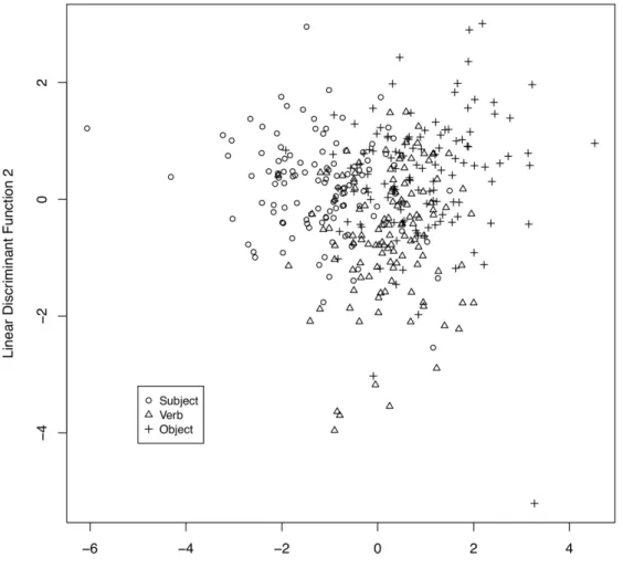
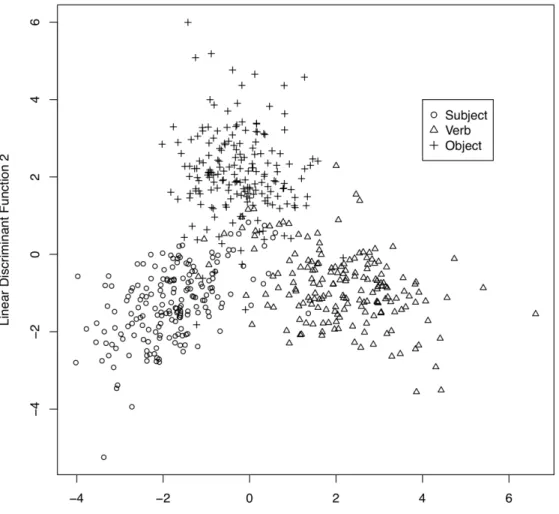
p < .001, indicating that the acoustic predictors could also differentiate verb focus from object focus (see Figure 2). Leave-one-out classification correctly classified 67% of the productions. The model correctly classified subject focus 76% of the time, verb focus 58% of the time, and object focus 66% of the time. Table 3 presents the standardized canonical discriminant function coefficients of the model.7
6Wilks's lambda is a measure of the distance between groups on means of the independent variables, and is
computed for each function. It ranges in size from 0-1; lower values indicate a larger separation between groups. The extent to which the model can effectively discriminate a new set of data is simulated by a leave-one-out classification, in which the acoustic data from each production are iteratively removed from the dataset, the model is computed, and the left-out case is classified by the resultant functions.
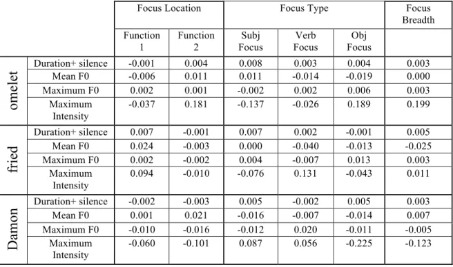
7 The coefficients in Table 3 indicate which acoustic features best discriminate focus location, such that
larger absolute values indicate a greater contribution of that feature to discrimination. For example, inspection of the plot in Figure 2 and the coefficients in the Focus Location columns of Table 3 shows that the acoustic features of Damon score around zero, or lower, on the first function (0.002, 0.001, 0.01, and -0.06) and around zero on the second function (-0.003, 0.021, -0.016, -0.101). Fried shows a different pattern; specifically, the acoustic features of fried have coefficients around zero for the first function, and negative coefficients for function 2. Finally, omelet shows a third pattern: its acoustic correlates are centered around zero on Function 1, but are high on Function 2.
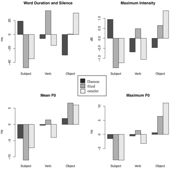
Figure 3 graphically presents the mean values of the four features, demonstrating that across all three focus locations the intended focus location is produced with the highest maximum intensity, the longest duration and silence, and the highest relative F0.
Focus Location Focus Type Focus Breadth Function 1 Function 2 Subj Focus Verb Focus Obj Focus Duration+ silence -0.001 0.004 0.008 0.003 0.004 0.003 Mean F0 -0.006 0.011 0.011 -0.014 -0.019 0.000 Maximum F0 0.002 0.001 -0.002 0.002 0.006 0.003
om
el
et
Maximum Intensity -0.037 0.181 -0.137 -0.026 0.189 0.199 Duration+ silence 0.007 -0.001 0.007 0.002 -0.001 0.005 Mean F0 0.024 -0.003 0.000 -0.040 -0.013 -0.025 Maximum F0 0.002 -0.002 0.004 -0.007 0.013 0.003fr
ied
Maximum Intensity 0.094 -0.010 -0.076 0.131 -0.043 0.011 Duration+ silence -0.002 -0.003 0.005 -0.002 0.005 0.003 Mean F0 0.001 0.021 -0.016 -0.007 -0.014 0.007 Maximum F0 -0.010 -0.016 -0.012 0.020 -0.011 -0.005Da
mo
n
Maximum Intensity -0.060 -0.101 0.087 0.056 -0.225 -0.123Table 3: Standardized canonical coefficients of the discriminant functions computed for Experiment 1.
Figure 2: Separation of focus locations on two discriminant functions in Experiment 1. The figure illustrates an effective discrimination among the three groups. Productions of subject focus are clustered in the upper left quadrant; productions of verb focus are clustered in the lower half of the plot; productions of object focus are clustered in the upper right quadrant.
Figure 3: Means of the four discriminating acoustic features of productions of Subject, Verb, and Object focus for Experiment 1.
Focus type
To determine how well the acoustic features could differentiate the type of focus (i.e. non-contrastive vs. contrastive) in speakers’ productions, we computed three models in which the 12 acoustic predictors were used to discriminate between two focus type groups. The three models investigated differences between non-contrastive and contrastive focus at the three focus locations: subject, verb, and object.
Focus Type – Subject Position
The overall Wilks’s Lambda was not significant, Λ = .898, χ2(12) = 11.95 p = .45, indicating that the acoustic features could not discriminate between non-contrastive and
Damon fried omelet
contrastive focus. Because the overall model is not significant, we do not present the scores of the specific acoustic features or the classification statistics here or in the analyses below.
Focus Type – Verb Position
The overall Wilks’s Lambda was not significant, Λ = .851, χ2(12) = 17.92 p = .12,
indicating that the acoustic features could not discriminate between non-contrastive and contrastive focus.
Focus Type – Object Position
The overall Wilks’s Lambda was significant, Λ = .82, χ2(12) = 22.63 p < .05, indicating that the acoustic features could discriminate between non-contrastive and contrastive focus above chance level. Leave-one-out classification correctly classified 59% of the productions. The model correctly classified non-contrastive focus 59% of the time, and contrastive focus 59% of the time.
The coefficients in the Object Focus column of Table 3 indicate that intensity and mean F0 contribute most to classification. Figure 4 graphically presents the mean values
of the four features, demonstrating that contrastive focus is produced with a higher maximum intensity, a longer duration and silence, and higher maximum F0. Non-contrastive focus is produced with a higher mean F0.
Figure 4: Values for non-contrastive focus and contrastive focus type on the four discriminating acoustic features when the direct object “omelet” is focused in Experiment 1.
Wide Focus vs. Narrow Focus
To determine how well the acoustic features could differentiate focus breadth, we computed a model in which the 12 critical predictors were used to discriminate between productions where the entire sentence was focused and productions where the object was non-contrastively or contrastively focused.
The overall Wilks’s Lambda was significant, Λ = .75, χ2(12) = 47.83, p < .001,
indicating that the acoustic features could successfully discriminate between conditions where the entire event is focused and conditions where the object is narrowly focused.
Damon fried omelet
Leave-one-out classification correctly classified 72% of the productions. The model correctly classified wide focus 67% of the time, and narrow focus 74% of the time.
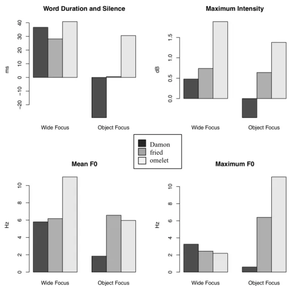
The standardized canonical discriminant function coefficients in the Focus Breadth column of Table 3 indicate that maximum intensity contributes most to focus breadth classification. Figure 5 graphically presents the mean values of the four features, demonstrating that wide focus is produced with a more uniform duration + silence and maximum F0 across the sentence than object focus. Wide focus is also produced with a more uniform, though overall greater, intensity than object focus.
Figure 5: Values for wide focus vs. narrow object focus on the four discriminating acoustic features in Experiment 3.
Discussion
Damon fried omelet
Focus Location
The results demonstrate that speakers consistently provide acoustic cues which disambiguate focus location. Specifically speakers indicated focus with increased duration, higher intensity, higher mean F0, and higher maximum F0. Furthermore, these results are consistent with the pattern reported in Eady & Cooper (1986), such that the word preceding a focused word is less prominent (produced with shorter duration, lower intensity and lower F0) than the focused word, and the word following the focused word is less prominent than the word preceding the focused word. Previous studies (Eady et al., 1986; Rump and Collier, 1986) have reported this reduction in acoustic prominence following focused elements as being mainly indicated by lower F0 on the post-focal words, though in our data we also find evidence of this reduction in measures of duration and intensity.
Focus Type
The results from Experiment 1 indicate that in semi-naturalistic productions speakers do not systematically differentiate between different focus types (focused elements which have explicit contrast sets in the discourse and those which do not). Specifically, at two out of three sentence positions, a discriminant function analysis could not successfully classify speakers’ productions of contrastively vs. non-contrastively focused elements. The observation that speakers successfully discriminated contrastive and non-contrastive focus in object position, but not in subject or verb positions, is perhaps suggestive, but is likely due to a lack of experimental power, a limitation which will be addressed in Experiment 2.
Focus Breadth
The results from Experiment 1 demonstrate that speakers do systematically mark focus breadth prosodically. Narrow object focus is produced with the highest maximum F0, longest duration, and maximum intensity of the object noun, relative to the other
words in the sentence. For wide focus, the acoustic features are more similar across the sentence; only intensity and mean F0 are higher on the object than on the other words in the sentence. These differences are subtle, but sufficient for the model to successfully discriminate the productions.
The fact that the model failed to systematically classify productions by focus type (with the exception of the object position), while achieving high accuracy in focus location and focus breadth indicates that speakers were not marking focus type with prosody in Experiment 1. However, the method used to elicit productions did not require that subjects be aware of the information structure ambiguity of the materials. Evidence from other production studies suggests that speakers may not prosodically disambiguate ambiguous productions if they are not aware of the ambiguity. Albritton, McKoon, and Ratcliff (1996), for example, demonstrated that speakers did not disambiguate
syntactically ambiguous constructions like “Dave and Pat or Bob” unless they were aware of the ambiguity (see also Snedeker and Trueswell, 2003, but cf. Kraljic and Brennan, 2005, and Schafer, Speer, Warren, and White, 2000, for evidence that speakers do disambiguate syntactically ambiguous structures even in the absence of ambiguity awareness). Experiment 2 was designed to be a stronger test of speakers’ ability to differentiate focus location, focus type, and focus breadth. We used materials similar to those in Experiment 1, with two important methodological modifications. First, instead of producing the answers to questions with no feedback, the speaker’s task now involved trying to enable the answerer to choose the question that s/he was answering from a set of possible questions. Moreover, we introduced feedback so that the speaker would always know whether his/her partner had chosen the correct answer. Second, we changed the design from a between- to a within-subjects manipulation. This ensured that speakers
were aware of the manipulation, as they were producing the same answer seven times with explicit instructions to differentiate their answers for their partner.
In addition to making the speaker’s task explicit, the new design also allowed us to analyze the subset of the productions for which the listeners could successfully identify the question-type and which therefore contain sufficient information for differentiating utterances along the three relevant dimensions of information structure.
Experiment 2
MethodParticipants
Seventeen pairs of participants were recorded for this experiment. Subjects were MIT students or members of the surrounding community. All reported being native speakers of American English. None had participated in Experiment 1. Participants were paid for their participation.
Materials
The materials had the same structure as those from Experiment 1, though the critical words differed. Specifically, a larger set of names and a wider variety of temporal adverbs were used, and some verbs and objects differed from Experiment 1. Unlike Experiment 1, each subject pair was presented with all seven versions of each of 14 items, according to a full within-subjects within-items design. All materials can be found in Appendix B.
Procedure
Two participants sat at computers in the same room such that neither could see the other’s screen. One participant was the speaker, and the other was the listener. Speakers were told that they would be producing answers to questions out loud for their partners
(the listeners), and that the listeners would be required to choose which question the speaker was answering from a set of seven choices.
At the beginning of each trial, the speaker was presented with a question on the computer screen to read silently. After pressing a button, the answer to the question appeared below the question, accompanied by a reminder to the speaker that s/he would only be producing the answer aloud, and not the question. Following this, the speaker had one more chance to read the question and answer, and then he/she was instructed to press a key to begin recording (after being told by the listener that he/she is ready), to produce the answer, and then to press another key to stop recording.
The listener sat at another computer, and pressed a key to see the seven questions that s/he would have to choose his/her answer from. When s/he felt familiar with the questions, s/he told the speaker s/he was ready. After the speaker produced a sentence out loud for the listener, the listener chose the question s/he thought the speaker was answering. If the listener answered incorrectly, his/her computer produced a buzzer sound, like the sound when a contestant makes an incorrect answer on a game show. This cue was included to ensure that speakers knew when their productions did not contain enough information for the listener to choose the correct answer.8
Results – Production
Two speaker-listener pairs were excluded as the Listener did not achieve comprehension accuracy greater than 20%. One further pair was excluded as one member was not a native speaker of American English. Finally, another pair of subjects was excluded because they did not take the task seriously, and produced unnaturally emphatic contrastive accents, often shouting the target word, and laughing while doing
8
In early pilots in which there was no feedback for incorrect responses, we observed that listeners were at chance in choosing the correct question.
so. These exclusions left a total of 13 pairs of participants whose responses were analyzed.
Sixty-seven of the 1274 trials (5%) were excluded because (a) the speaker failed to produce the correct words, (b) the speaker was disfluent, or (c) the production was poorly recorded. Analyses were performed on all trials, and on the subset of trials for which the listener correctly identified the question. The results were very similar in the two analyses. For brevity of presentation, we present results from analyses conducted on the correct trials (n = 660, 55%). The productions from Experiment 2 were analyzed using the acoustic features chosen in the feature-selection procedure described in
Experiment 1. All analyses were performed on the residual values of these features, after removing speaker and item variance with the method described in Experiment 1.
Focus Location
The overall Wilks’s lambda was significant, Λ = .085, χ2(24) = 1335, p < .001, indicating that the acoustic features could differentiate subject focus from verb and object focus. In addition, the residual Wilks’s lambda was significant, Λ = .306, χ2(11) = 641, p
< .001, indicating that the acoustic features could also discriminate verb focus from object focus (see Figure 6).
Leave-one-out classification correctly classified 93% of the productions. For individual levels of focus location, the discriminant function correctly classified subject focus 94% of the time, verb focus 90% of the time, and object focus 95% of the time.
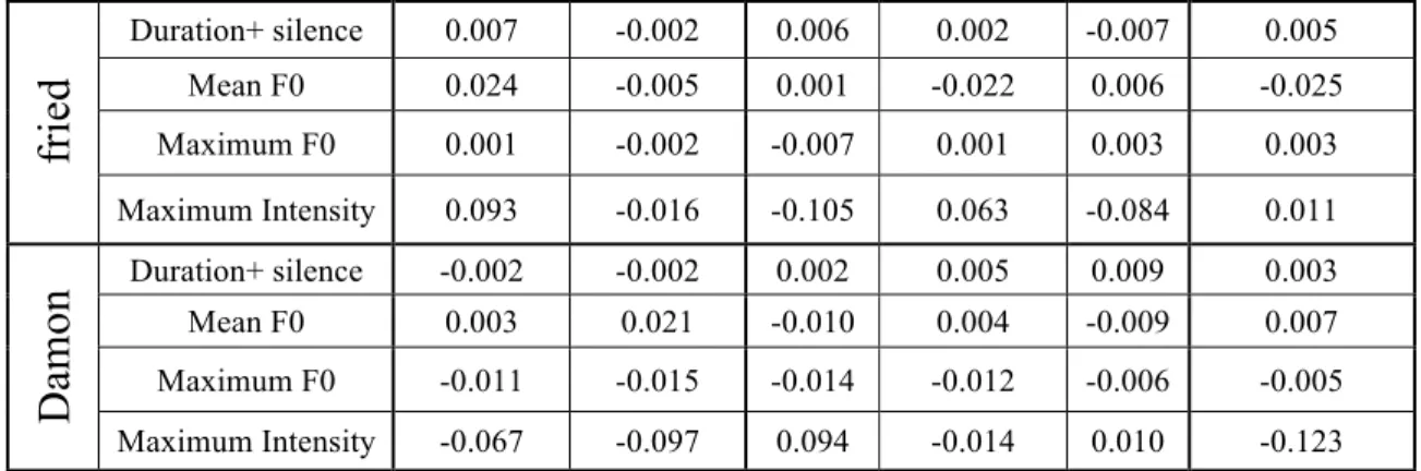
The standardized canonical coefficients in the first two columns of Table 4 indicate that the acoustic features contributing most to the discrimination of focus location are once again mean F0 and maximum intensity, though the other two features are also contributing. In fact, inspection of the acoustic feature means in Figure 7
demonstrate that the highest value of every acoustic feature is associated with the intended focused item, with the exception of mean F0 when the subject is focused.
Figure 6: Separation of focus locations on two discriminant functions for Experiment 2. The figure illustrates an effective discrimination among the three groups. Productions of subject focus are clustered in the lower left quadrant of the plot; productions of verb focus are clustered in the lower right quadrant; productions of object focus are clustered in the lower half.
Focus Location Focus Type Focus Breadth Function 1 Function 2 Subject Focus Verb Focus Object Focus
Duration+ silence -0.001 0.004 0.004 0.006 0.003 0.003 Mean F0 -0.006 0.011 -0.003 0.005 -0.023 0.000 Maximum F0 0.002 0.001 0.004 -0.009 -0.003 0.003
om
el
et
Maximum Intensity -0.025 0.183 -0.052 -0.171 0.012 0.199Duration+ silence 0.007 -0.002 0.006 0.002 -0.007 0.005 Mean F0 0.024 -0.005 0.001 -0.022 0.006 -0.025 Maximum F0 0.001 -0.002 -0.007 0.001 0.003 0.003
fr
ied
Maximum Intensity 0.093 -0.016 -0.105 0.063 -0.084 0.011 Duration+ silence -0.002 -0.002 0.002 0.005 0.009 0.003 Mean F0 0.003 0.021 -0.010 0.004 -0.009 0.007 Maximum F0 -0.011 -0.015 -0.014 -0.012 -0.006 -0.005Da
mo
n
Maximum Intensity -0.067 -0.097 0.094 -0.014 0.010 -0.123Table 4: Standardized canonical coefficients of all discriminant functions computed for Experiment 2.
Figure 7: Means of the four discriminating acoustic features of productions of Subject, Verb, and Object focus for Experiment 2.
Damon fried omelet
Focus Type
Focus Type – Subject Position
The overall Wilks’s Lambda was significant, Λ = .633, χ2(12) = 81.41, p<.001, indicating that the acoustic features could discriminate between non-contrastive and contrastive focus better than chance. Leave-one-out classification correctly classified 75% of the productions. The model correctly classified non-contrastive focus 78% of the time, and contrastive focus 71% of the time.
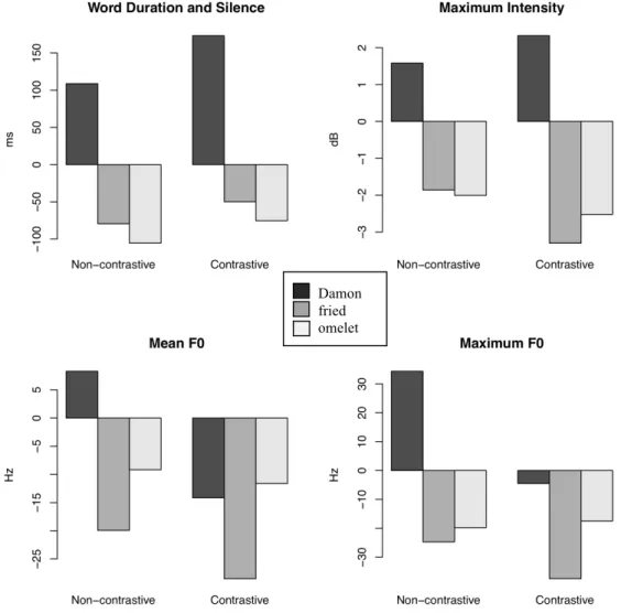
The standardized canonical discriminant function coefficients in Table 4 indicate that maximum intensity at all three locations (i.e. large intensity differences between the subject and verb and the subject and object) contributes most to classification. Figure 8 graphically presents the mean values of the four features, demonstrating that, in addition to intensity differences, contrastive focus is produced with longer duration and silence, as well as lower mean and maximum F0.
Focus Type – Verb Position
The overall Wilks’s Lambda was significant, Λ = .654, χ2(12) = 72.27, p< .001,
indicating that the acoustic features could discriminate between non-contrastive and contrastive focus better than chance. Leave-one-out classification correctly classified 72% of the productions. The model correctly classified non-contrastive focus 70% of the time, and contrastive focus 75% of the time.
The standardized canonical discriminant function coefficients in Table 4 indicate that, once again maximum intensity contributes most to classification. Figure 9
graphically presents the mean values of the four features, demonstrating that contrastive focus is produced with a higher maximum intensity, and a longer duration and silence, than non-contrastive focus. Once again, non-contrastive focus is produced with higher mean and maximum F0 than contrastive focus.
Focus Type – Object Position
The overall Wilks’s Lambda was significant, Λ = .793, χ2(12) = 41.3, p<.001,
indicating that the acoustic features could discriminate between non-contrastive and contrastive focus better than chance. Leave-one-out classification correctly classified 67% of the productions. The model correctly classified non-contrastive focus 69% of the time, and contrastive focus 66% of the time.
The standardized canonical discriminant function coefficients in Table 4 indicate that contrastive focus is most strongly associated with lower mean F0. Figure 10
graphically presents the mean values of the four features, demonstrating that contrastive focus is produced with a lower mean and maximum F0 than non-contrastive focus.
Figure 8. Values for non-contrastive focus vs. contrastive focus on the four discriminating acoustic features when “Damon” is focused in Experiment 2.
Damon fried omelet
Figure 9. Values for non-contrastive focus vs. contrastive focus on the four discriminating acoustic features when “fried” is focused in Experiment 2.
Damon fried omelet
Figure 10. Values for non-contrastive focus vs. contrastive focus on the four discriminating acoustic features when “omelet” is focused in Experiment 2. Wide Focus vs. Narrow Focus
The overall Wilks’s Lambda was significant, Λ = .59, χ2(12) = 148, p < .001,
indicating that the acoustic features could differentiate between wide focus and narrow object focus. Leave-one-out classification correctly classified 84% of productions; wide focus was correctly classified 77% of the time, and object focus was correctly classified 88% of the time.
The standard canonical coefficients in the “Focus Breadth” column of Table 4 indicate that the maximum intensity of each of the target words contributes most strongly to the discrimination of focus breadth. Although intensity is contributing most strongly to classification, inspection of the acoustic means in Figure 11 indicates that wide focus
Damon fried omelet
is marked by lesser prominence on the object, reflected in shorter duration, lower F0, and lower intensity; conversely, narrow object focus is marked by greater prominence on the object, reflected in longer duration, higher F0, and higher intensity.
Figure 11: Values for wide vs. narrow object focus on the four discriminating acoustic features in Experiment 2.
Damon fried omelet
Results – Perception
Figure 12. Percentage of Listeners’ condition choice by intended sentence type for Experiment 2.
Listeners’ choices of question sorted by the intended question are plotted in Figure 12. Listeners’ overall accuracy was 55%. To determine whether listeners were able to determine the speaker’s intended sentence meaning, we compared each subject's responses to chance performance. Specifically we assessed, for focus location and focus type, whether each subject's proportion of correct responses exceeded chance; wide focus productions were excluded from the analysis, so that chance performance for focus
location was .33, and chance performance for focus type was .5. Results demonstrated that listeners were able to successfully identify focus location: all 13 subjects’
performance significantly exceeded chance performance, p = .05, two-tailed. However, listeners were unable to successfully identify focus type: only three of 13 subjects performed at above-chance levels (based on the binomial distribution), p = .05, two-tailed. To investigate focus breadth, we assessed, for wide focus and narrow object focus separately, whether each subject's proportion of correct responses exceeded chance. For these analyses, we excluded subject and verb focus productions, so that chance
performance was .33 for wide focus, and .67 for narrow object focus. Results
demonstrated that listeners were moderately successful at identifying focus breadth: six of 13 subjects identified wide focus at rates above chance, and nine out of 13 subjects identified narrow object focus at levels above chance p = .05, two-tailed.
Discussion
The production results replicated the two main findings from Experiment 1, and provided evidence for acoustic discrimination of focus type across sentence positions as well. First, these results demonstrated that focused elements have longer durations than non-focused elements, incur larger F0 excursions, are more likely to be followed by silence, and are produced with greater intensity. Second, speakers consistently differentiate between wide and narrow focus by producing the object in the latter case with higher F0, longer duration, and greater intensity. Specifically, although object focus was indicated by increased duration, higher intensity, and higher F0 on the object than on the subject or the verb, wide focus was indicated by comparatively greater duration, higher intensity, and higher F0 on the subject and the verb, and shorter duration, lower intensity, and lower F0 on the object. These results are consistent with those obtained by Baumann et
al. (2006), who demonstrated that narrow focus on an element was indicated with longer duration and a higher F0 peak than wide focus on an event encompassing that element.
Most importantly, although speakers in Experiment 1 did not differentiate conditions with and without an explicit contrast set for the focused element (except for the object position), these conditions were differentiated by speakers in Experiment 2, at every syntactic position. There are two possible interpretations of this difference. First, in Experiment 1, speakers produced only four versions of each of the seven conditions, whereas speakers in Experiment 2 and 3, reported below, produced 14 versions of each of the seven conditions, resulting in greater power in the latter two experiments. The fact that, in Experiment 2, speakers successfully discriminated contrastive and
non-contrastive focus in all three positions, suggests that the lack of such an effect in Experiment 1 could be due to a lack of power.
As mentioned above, the difference in the findings between Experiments 1 and 2 is also consistent with results from Allbritton et al. (1996) and Snedeker and Trueswell (2003) who demonstrated that speakers do not disambiguate syntactically ambiguous sentences with prosody unless they are aware of the ambiguity. The current results demonstrate a similar effect for acoustic prominence, such that speakers do not differentiate two kinds of acoustically prominent elements (contrastively vs. non-contrastively focused elements) unless they are aware of the information structure ambiguity in the structures they are producing.
The discriminant analyses indicated that contrastively focused words were produced with longer durations and higher intensity than non-contrastively focused words, but that non-contrastively focused words were produced with higher F0 than contrastively focused words. This latter finding is surprising when compared to some previous studies. For example, Ladd & Morton (1997) found that higher F0 and larger
F0 range is perceived as more ‘emphatic’ or ‘contrastive’ by listeners. Similarly, Ito and Speer (2008) demonstrated that contrastively focused words were produced with higher F0 than non-contrastive ones. Given the unexpected results, we inspected individual pitch tracks to more closely observe the F0 patterns across the entire utterances. The pitch tracks presented in Figure 13 were generated from the productions of a typical speaker, and they exemplify the higher F0 observed for non-contrastive focus than contrastive focus in the subject position (A vs. B) and verb position (C vs. D).
Contrastive focus on the object is realized with the same F0 as non-contrastive focus on the object (E vs. F).
Damon fried an omelet yesterday Non-Contrastive Given Given
50 300 100 150 200 250 Pitch (Hz) Time (s) 0 1.433
A. Non-contrastive Subject Focus
B. Contrastive Subject Focus
C. Non-contrastive Verb Focus
Damon fried an omelet yesterday Contrastive Given Given
50 300 100 150 200 250 Pitch (Hz) Time (s) 0 1.81
Damon fried an omelet yesterday Given Non-Contrastive Given
50 300 100 150 200 250 Pitch (Hz) Time (s) 0 1.514
Damon fried an omelet <SIL> yesterday Given Contrastive Given
50 300 100 150 200 250 Pitch (Hz) Time (s) 0 2.377
D. Contrastive Verb Focus
E. Non-contrastive Object Focus
F. Contrastive Object Focus
Figure 13. Pitch tracks for non-contrastive and contrastive subject focus, non-contrastive and contrastive verb focus, and non-contrastive and contrastive object focus,
respectively, from a typical speaker from Experiment 2.
Note that our finding that non-contrastive focus is realized with higher F0 than contrastive focus is still consistent with the claim that contrastive focus is more
prominent than non-contrastive focus. As the graphs in Figures 8-10, and the pitch tracks in Figure 13 indicate, although contrastive elements were consistently produced with lower pitch, they were also consistently produced with longer durations and greater
Damon fried an omelet yesterday
Given Given Non-Contrastive 50 300 100 150 200 250 Pitch (Hz) Time (s) 0 1.582
Damon fried an omelet yesterday
Given Given Contrastive 50 300 100 150 200 250 Pitch (Hz) Time (s) 0 2.188