HAL Id: hal-00727104
https://hal.archives-ouvertes.fr/hal-00727104
Submitted on 16 Sep 2012
HAL is a multi-disciplinary open access
archive for the deposit and dissemination of
sci-entific research documents, whether they are
pub-lished or not. The documents may come from
teaching and research institutions in France or
abroad, or from public or private research centers.
L’archive ouverte pluridisciplinaire HAL, est
destinée au dépôt et à la diffusion de documents
scientifiques de niveau recherche, publiés ou non,
émanant des établissements d’enseignement et de
recherche français ou étrangers, des laboratoires
publics ou privés.
An automatic correction of Ma’s thinning algorithm
based on P -simple points
Christophe Lohou, Julien Dehos
To cite this version:
Christophe Lohou, Julien Dehos. An automatic correction of Ma’s thinning algorithm based on P
-simple points. Journal of Mathematical Imaging and Vision, Springer Verlag, 2010, 36 (1), pp.54-62.
�10.1007/s10851-009-0170-1�. �hal-00727104�
An automatic correction of Ma’s thinning algorithm
based on P -simple points
Christophe LOHOU and Julien DEHOS
1 Laboratoire d’Algorithmique et Image de Clermont, Universit´e d’Auvergne, France 2Laboratoire d’Informatique du Littoral, Universit´e du Littoral Cˆote d’Opale, France
Abstract
The notion of P -simple points has been introduced by Bertrand to conceive parallel thinning algorithms. In ’A 3D fully parallel thinning algorithm for generating medial faces’, Ma has proposed an algorithm for which there exists objects whose topology is not preserved. In this paper, we propose a new application of P -simple points: to automatically correct Ma’s algorithm.
Keywords: topology preservation; thinning algorithm correction; surface skeleton
1
Introduction
In the image processing framework, thinning is a technique which extracts skeletons from objects. Such a repre-sentation has the advantage of being compact while conserving important features of objects like topology and ge-ometry. Thinning has many applications such as compression, analysis and recognition [Reniers and Telea(2007)]. In a binary image, objects are represented by black points. The complement is represented by white points. Thinning consists of changing black points to white. It is generally done in successive iterations of deletions. Removing a point should preserve certain properties like topology. This leads to the essential notion of a simple point: a simple point is a point which can be removed without changing topology [Kong and Rosenfeld(1989)]. The literature gives several kinds of 3D thinning algorithms. Parallel thinning algorithms proceed by re-moving black points in parallel. Implemented on appropriate computers, such algorithms can efficiently achieve thinning. The problem is that the notion of a simple point is not powerful enough to garantee topology preser-vation in this context. For example, consider an object made of two neighboring points. Both points are simple but removing them both does change topology. This problem cannot occur by sequential processing because the deletion of the first point makes the second point become non-simple. To solve this problem, Bertrand has proposed the notion of P -simple points [Bertrand(1995a)]: a point of a set P is P -simple if it is simple when any subset of P is removed. Parallel thinning algorithms removing P -simple points have been proposed [Bertrand(1995b), Lohou and Bertrand(2004), Lohou and Bertrand(2005), Lohou and Bertrand(2007)]. Such algorithms have remarkable topology-preserving property.
In this paper we propose another application of P -simple points: ensuring topology preservation of an existing parallel thinning algorithm. In [Ma(1995)], Ma proposes a 3D parallel thinning algorithm. This algorithm is one of the few thinning algorithms able to preserve surfaces and is used as a reference [Pal´agyi(2008), Lohou and Bertrand(2007)]. In [Lohou(2008)], one of the authors gives an object whose topology is not preserved by Ma’s algorithm. This proves that the algorithm fails to preserve topology, which it should do. Here, we propose a topology preserving algorithm by using P -simple points to repair Ma’s algorithm. As far as we know, this is the first time P -simple points are used to automatically correct an image operator.
This paper is organized as follows. Section 2 gives some basic notions of Digital Topology and presents P-simple points. Section 3 shows how to use P -simple points in a thinning algorithm. In section 4, we propose such an algorithm to correct Ma’s. Section 5 gives some results and section 6 concludes.
2
Basic notions of Digital Topology
2.1
Neighborhoods and connected components
A point x ∈ Z3
is defined by (x1, x2, x3) with xi ∈ Z. We consider the three neighborhoods: N26(x) = {x′ ∈ Z3: max[|x1− x′1|, |x2− x′2|, |x3− x′3|] ≤ 1},
N6(x) = {x′∈ Z3
: |x1−x′1|+|x2−x′2|+|x3−x′3| ≤ 1}, and N18(x) = {x′∈ Z3
: |x1−x′1|+|x2−x′2|+|x3−x′3| ≤ 2} ∩ N26(x). We define Nn(x) = N∗ n(x) \ {x}. We call respectively 6-, 18-, 26-neighbors of x the points of
(a) (b)
Figure 1: (a): The 6-neighbors (triangles), 18-neighbors (diamonds) and 26-neighbors (crosses) of x. (b): Axis and orientations.
(a) (b) (c) (d)
Figure 2: Simple points and P -simple points. Black points represent the object X. White points and hidden points represent the complement X. (a): x is 26-simple for X. (b): x is not 26-simple for X. In (c) and (d), black squares represent P and black discs represent X \ P . (c): x is P -simple for X. (d): x is not P -simple for X.
N∗
6(x), N18(x) \ N∗ 6∗(x), N26(x) \ N∗ 18(x). Such points are represented in Fig. 1 (a). Let X ⊆ Z∗ 3
. The points belonging to X (resp. X, the complement of X in Z3
) are called black points (resp. white points). Axis and orientations used in this paper are given in Fig. 1 (b).
Two points x and y are said to be n-adjacent if y ∈ N∗
n(x) (n = 6, 18, 26). An n-path is a sequence of points x0, . . . , xk, with xi n-adjacent to xi−1 and 1 ≤ i ≤ k. If x0= xk, the path is closed. Let X ⊆ Z3. Two points x∈ X and y ∈ X are n-connected if they can be linked by an n-path included in X. The equivalence classes relative to this relation are the n-connected components of X. The presence of an n-hole is detected whenever there is a closed n-path in X that cannot be deformed, in X, into a single point (see [Kong(1989)], for further details). In order to have a correspondence between the topology of X and that of X, we have to consider two different kinds of adjacency for X and for X [Kong and Rosenfeld(1989)]: if we use an n-adjacency for X, we have to use another n-adjacency for X. In this paper, we only consider (n, n) = (26, 6).
2.2
Simple points and topological numbers
Let X ⊆ Z3
. A point x ∈ X is said to be n-simple for X if its deletion does not “change the topology” of the image, in the sense that there is a bijection between the components and the holes of X and X and the ones of X\ {x} and X ∪ {x} (see [Kong(1989)] for a precise definition). In the following, we write x is simple instead of x is simple for X. In Fig. 2 (a), we may verify that x is simple. In Fig. 2 (b), X is a single connected component whereas X \ {x} is made of two connected components ({a, c} and {b}), therefore the topology of X is not preserved by the deletion of x, i.e. x is not simple.
The set composed of all n-connected components of X is denoted by Cn(X). The set of all n-connected components of X and n-adjacent to a point x is denoted by Cx
n(X). Let #X denote the number of elements which belong to X. The topological numbers relative to X and x are the two numbers [Bertrand(1994)]: T6(x, X) = #Cx
6(N18(x) ∩ X) and T26(x, X) = #C∗ x
26(N26(x) ∩ X) (in fact, T26(x, X) = #C26(N∗ 26(x) ∩ X), since any 26-∗ connected component of black points in N26(x) is inevitably 26-adjacent to x). These numbers lead to a very∗ concise characterization of 3D simple points [Malandain and Bertrand(1992), Bertrand and Malandain(1994)]: x∈ X is 26-simple if and only if T26(x, X) = 1 and T6(x, X) = 1. For example, in Fig. 2 (a), the points of N26(x) ∩ X (resp. N∗ 18(x) ∩ X) make a single 26-connected (resp. 6-connected and 6-adjacent to x) component.∗ Thus (T26(x, X), T6(x, X)) = (1, 1); therefore x is simple. In Fig. 2 (b), N26(x) ∩ X is constituted by two∗
26-connected components ({a, c} and {b}). N18(x) ∩ X is made of a single 6-connected component 6-adjacent∗ to x. Thus, we have, (T26(x, X), T6(x, X)) = (2, 1); therefore x is not simple.
2.3
P -simple points
This section recalls the definition of P -simple points and several properties of such points [Bertrand(1995a)]. In the following, we consider a subset X of Z3
, a subset P of X and a point x of P .
Definition 1 The point x is P -simple for X if for each subset S of P \ {x}, x is 26-simple for X \ S.
For example, in Fig. 2 (c), P = {x, a}. We may verify that x is simple for X \ {a}; therefore x is P -simple. In Fig. 2 (d), P = {x, a}. With S = {a}, we may verify that x is not simple for X \ S; therefore x is not P-simple.
We have the remarkable property that any algorithm removing subsets composed solely of P -simple points is garanteed to keep the topology unchanged [Bertrand(1995a)].
The following proposition permits to locally characterize P -simple points [Bertrand(1995c)]. Proposition 1 The point x is P -simple if and only if:
T26(x, X \ P ) = 1, T6(x, X) = 1,
∀y ∈ N26(x) ∩ P, ∃z ∈ X \ P such that z is 26-adjacent to x and to y,∗ ∀y ∈ N6∗(x) ∩ P, ∃z ∈ X and∃t ∈ X such that {x, y, z, t} is a unit square.
For example, in Fig. 2 (c), x is P -simple because it concurs with the four conditions of Proposition 1. In Fig. 2 (d), x is not P -simple because the first condition is not satisfied (T26(x, X \ P ) = 2). In both examples, Proposition 1 makes it possible to consider only a few points around x to determine whether x is P -simple or not.
3
Thinning algorithms based on P -simple points
Let us consider an algorithm which removes P -simple points in parallel, in successive iterations. Since some points are deleted during an iteration, this algorithm thins objects. A skeleton is obtained when no more points can be removed. As shown in the previous section, removing subsets composed of solely P -simple points guarantees to keep the topology unchanged. Consequently, topology preservation, which is one of the most important features of a thinning algorithm, is automatically proved for such algorithms.
Algorithm 1: P-SimpleThinningAlgorithm(X, C) → X
1: repeat
2: {parallel labelling of points which belong to P }
3: P ← ∅
4: foreach point x in X, in parallel, do
5: if xverifies the condition C then
6: put x in P 7: end if
8: end for
9: {parallel deletion of P -simple points} 10: foreach point x in P , in parallel, do 11: if xis P -simple for X then
12: delete x in X
13: end if
14: end for
15: untilno points are deletable
Algorithm 1 gives such an algorithm; where C denotes the condition a point x of X should satisfy to belong to P (the set of candidate points to deletion). Each iteration is composed of two passes. Thanks to P -simple points, the algorithm can examine points in parallel. Furthermore, using the local characterization of P -simple points (Proposition 1), the algorithm can consider limited neighborhoods. It is thus well-suited for parallel machines.
Algorithm 1 does not explain how to determine P (the set of candidate points for deletion). In [Bertrand(1995a)], Bertrand proposes that P contains the simple points of X to obtain a certain kind of skeleton.
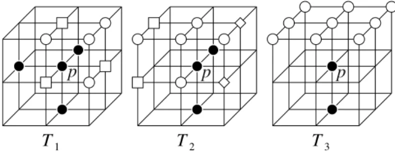
Figure 3: The templates of Ma’s algorithm. A point p satisfies a template if each disc is a black point, each circle is a white point, at least one square is a white point and at least one diamond is a white point.
4
A new thinning algorithm correcting Ma’s algorithm
In the previous section, we have recalled how P -simple points can be used to conceive thinning algorithms. We now suggest a new application of P -simple points: to correct an existing thinning algorithm which fails to preserve topology. Indeed, a lot of parallel thinning algorithms (including Ma’s algorithm) are based on “local” templates. Basically, they consist of removing in parallel and in successive iterations, all the points matching one of the given templates. A skeleton is obtained when no more points can be removed. However, when a templates-based thinning algorithm is proposed, its topology preservation should be proven afterward. This is very difficult because it implies considering a great number of configurations in a greater neighborhood than the N26 neighborhood of the considered point. Thus, giving an analytical proof is difficult and computing the correctness of the algorithm cannot be done in reasonnable time using actual computers. That’s why an error can be made easily, when a templates-based thinning algorithm is conceived. This is what has occured with Ma’s algorithm. A correction could be made by changing the initial templates but, once again, proof has to be given, which leads us to the previously mentioned difficulties. In this section, we explain how to use P -simple points to correct, in a simple and effective manner, a templates-based thinning algorithm which fails to preserve topology.
4.1
Study of Ma’s algorithm
This algorithm has been proposed in [Ma(1995)]. It is a 3D parallel thinning algorithm based on templates requiring access of up to 30 points to decide whether a point is deletable or not.
In [Ma(1995)], Ma gives the following definitions and rules:
• A black point is called border point if it is 6-adjacent to a white point.
• Definition 1.1: Let p be a black point of a 3D image. Then p is called an edge point if p has exactly one black 26-neighbor in N26(p) or in any of the three orthogonal 3 × 3 planes containing p; p is called a∗
non-edge point if it is not an edge point.
• Suppose p is a point in a 3D image. Let s(p), w(p) and d(p) be the south, west and down neighbors of p, respectively.
• Rule 2.1: Suppose all four corners of a unit lattice square are to be deleted. Then the corner with the smallest sum of coordinates is preserved if and only if it is non-simple after the other three corners are deleted.
• Let Ω be the set of all rotations and reflections of all three configurations (shown in Fig. 3). For each element T of Ω, a black point p is said to satisfy T if [it satisfies the corresponding template and]1
all of the following conditions are satisfied:
pis a non-edge point,
if p is a north border point, then s(s(p)) is a black point, if p is a east border point, then w(w(p)) is a black point, if p is a up border point, then d(d(p)) is a black point. A black point p is said to satisfy Ω if p satisfies any element in Ω.
Using these definitions, Ma gives the Algorithm 2, denoted by Ma95.
This algorithm works by iterations. Each iteration is composed of two passes (find black points satisfying Ω; delete points not preserved by Rule 2.1). During a pass, points can be considered in parallel.
Algorithm 2: Ma95
1: repeat
2: parallel delete black point that satisfies Ω and is not preserved by Rule 2.1 3: untilno points are deleted
In [Lohou(2008)], it is shown that Ma’s algorithm does not always preserve topology. Now, we propose an algorithm which corrects this problem.
4.2
Our proposal
In section 3, we proposed a generic parallel thinning algorithm (Algorithm 1). First, this algorithm detects, in parallel, the points which verify a condition C. These points compose the set P . Then, the algorithm deletes P-simple points in parallel among the points of P .
To correct Ma’s algorithm, we propose to remove P -simple points in parallel in successive iterations where P is precisely the set of points which would be deleted by Ma’s algorithm. This is equivalent to Algorithm 1 where the condition C is “the point satisfies Ω and is not preserved by Rule 2.1”.
Checking Rule 2.1 for a point x requires us to determine if some neighbors of x are to be deleted. This can be done by checking whether they satisfy Ω or not. This method means accessing a larger neighborhood of x (see [Lohou and Bertrand(2004)] for further details). To avoid this, we can first find the points that satisfy Ω and, in another pass, determine which ones are preserved by Rule 2.1. This algorithm, denoted by LD09, is given in Algorithm 3.
Algorithm 3: LD09(X) → X
1: repeat
2: {parallel labelling of points which belong to P′} 3: P′← ∅
4: foreach point x in X, in parallel, do
5: if xsatisfies Ω then
6: put x in P′ 7: end if
8: end for
9: {parallel application of Rule 2.1}
10: P ← ∅
11: foreach point x in P′, in parallel, do
12: if xis not preserved by Rule 2.1 in P′ then
13: put x in P
14: end if
15: end for
16: {parallel deletion of P -simple points} 17: foreach point x in P , in parallel, do
18: if xis P -simple for X then
19: delete x in X 20: end if
21: end for
22: untilno points are deletable
LD09 is indeed a correction of Ma95. First, it removes P -simple points only, which ensures topology preservation. And finally, it can delete only the same points as Ma95. This use of P -simple points implies that LD09 preserves topology. On the contrary, a correction based only on a modification of the initial templates would have required a difficult and error-prone proof of the topology preservation.
We may notice that other algorithms can be derived from LD09. For instance, Rule 2.1 may be checked in the same time as the P -simpleness, which makes it possible to bypass the specific pass. Another algorithm can be defined by letting P be the set of points which match the templates and then removing P -simple points which are non-edge points and non-border points. We are currently working on these points and a few other ones [DEHOS and LOHOU(2009)].
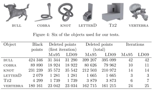
bull cobra knot letterD Tz2 vertebra Figure 4: Six of the objects used for our tests.
Object Black Deleted points Deleted points Iterations points (first iteration) (total)
Ma95 LD09 Ma95 LD09 Ma95 LD09 bull 424 346 31 344 31 290 399 207 395 099 42 42 cobra 89 890 18 924 18 922 80 626 79 962 10 11 knot 231 239 35 572 35 542 212 503 210 972 14 14 letterD 2 079 1 281 1 281 1 665 1 665 3 3 Tz2 4 299 1 739 1 739 3 879 3 873 6 7 vertebra 180 161 23 042 23 034 162 715 161 215 24 25 Table 1: Comparison between Ma95 and LD09 applied to the 6 objects depicted in Fig. 4.
5
Results
We have compared Ma’s algorithm and ours thanks to 5 small synthetic objects, 5 large objects obtained by voxelisation and 1 object obtained by medical imagery (see Table 1. Some of these objects are depicted in Fig. 4. We have found that 3 objects have the same number of deleted points with both algorithms (for instance, letterD and Tz2), 8 objects have more deleted points with Ma’s algorithm and no object has more deleted points with our algorithm. Furthermore, 6 objects have the same number of iterations with both algorithms (for instance, Bull), one object has more iterations with Ma’s algorithm and 4 objects have more iterations with our algorithm (for instance, vertebra).
If we apply these algorithms to the same object, we can get different results after the first iteration, because LD09removes some but not always all of the points removed by Ma95. Thus, the next iteration happens on different objects therefore the final results are difficult to compare. By its conception, our algorithm cannot delete more points of a given object than Ma’s algorithm, during one iteration (columns 3 and 4 of Table 1. According to our tests, our algorithm generally deletes less points and performs more iterations than Ma’s. However, we cannot prove anything from this. For example, as mentioned before, one object of our database is thinned by less iterations with our algorithm than with Ma’s.
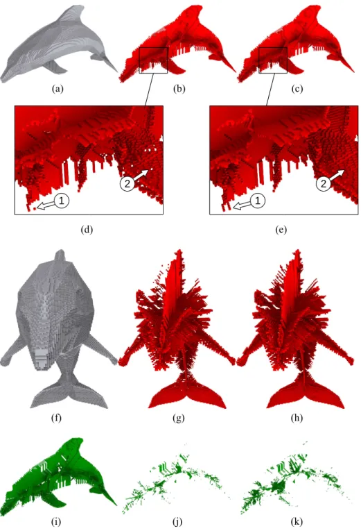
Fig. 5 shows the result of both algorithms applied to an object of the database. The initial object (a) is a dolphin obtained by voxelisation. The skeletons given by Ma’s algorithm (b) and ours (c) are quite similar. However, we can see on their respective close-ups (d) and (e), that Ma’s algorithm does not preserve the topology whereas ours does. For example, in (d), the stamp 1 depicts a voxel which is disconnected from the skeleton by Ma’s algorithm. In the same way, the stamp 2 shows a hole created by the algorithm. We can see on (e) that our algorithm does not have these problems. From another viewpoint (f), we can notice that, like Ma’s skeleton (g), our skeleton (h) presents medial faces. Finally, if the skeletons have common points (i), they also have points which are unique to themselves (j, k).
6
Conclusion
Up until now, P -simple points have been used to develop new topology-preserving thinning algorithms. In this paper, thanks to P -simple points, we have proposed an automatic correction of a templates-based thinning algorithm which fails to preserve topology. Like this latter, our algorithm allows us to extract medial-face skeletons. However, our algorithm ensures topology preservation. To our knowledge, it is the first time P -simple points are used for such an application. Our algorithm could be seen as a correcting patch for current applications using Ma’s algorithm.
Acknowledgments
We are grateful to Professor Gilles BERTRAND (ESIEE, Universit´e Marne-la-vall´ee, France) for our numerous discussions about P -simple points applied to thinning algorithms, to Romain JACQUINOT (IUT Le Puy-en-Velay, Universit´e d’Auvergne, France) for rendering the images of 4 and 5 and to Susan ARBON for help in preparing this paper.
1 2 1 2 (e) (c) (d) (j) (k) (i) (g) (h) (f) (b) (a)
Figure 5: Result of both algorithms applied to a same object. (a): Initial object (1 202 772 black points). (b): Skeleton obtained with Ma’s algorithm (1 153 121 deleted points in 60 iterations, 49 651 remaining points). (c): Skeleton obtained with our algorithm (1 150 230 deleted points in 61 iterations, 52 542 remaining points). (d): Close-up of (b). (e): Close-up of (c). (f): Another viewpoint of (a). (g): (b) from the same viewpoint as (f). (h): (c) from the same viewpoint as (f). (i): Intersection of (b) and (c) (45 967 points). (j): Difference between (b) and (c) (3 684 points). (k): Difference between (c) and (b) (6 575 points).
References
[Bertrand(1994)] Bertrand, G., 1994. Simple points, topological numbers and geodesic neighborhoods in cubic grids. Pattern Recognition Letters 15, 1003–1011.
[Bertrand(1995a)] Bertrand, G., 1995a. On P -simple points. In: Compte Rendu. Vol. 321 of S´erie I. Acad´emie des Sciences, Paris, pp. 1077–1084, (Computer Science/ Theory of Signals).
[Bertrand(1995b)] Bertrand, G., 1995b. P -simple points: A solution for parallel thinning. In: Actes du 5`eme colloque Discrete Geometry for Computer Imagery, DGCI’1995, Clermont-Ferrand, France. pp. 233–242. [Bertrand(1995c)] Bertrand, G., 1995c. Sufficient conditions for 3D parallel thinning algorithms. In: Conference
on Vision Geometry IV, San Diego, CA, USA. Vol. 2573. SPIE, Bellingham, WA, pp. 52–60.
[Bertrand and Malandain(1994)] Bertrand, G., Malandain, G., 1994. A new characterization of three-dimensional simple points. Pattern Recognition Letters 15, 169–175.
[DEHOS and LOHOU(2009)] DEHOS, J., LOHOU, C., 2009. Analysis of new thinning algorithms derived from Ma’s algorithm using P -simple points, in preparation.
[Kong(1989)] Kong, T., 1989. A digital fundamental group. Computer and Graphics 13 (2), 159–166.
[Kong and Rosenfeld(1989)] Kong, T., Rosenfeld, A., 1989. Digital topology: Introduction and survey. Com-puter Vision, Graphics and Image Processing 48, 357–393.
[Lohou(2008)] Lohou, C., 2008. Detection of the non-topology preservation of Ma’s 3D surface-thinning algo-rithm, by the use of P -simple points. Pattern Recognition Letters 29 (6), 822–827.
[Lohou and Bertrand(2004)] Lohou, C., Bertrand, G., 2004. A 3D 12-subiteration thinning algorithm based on P-simple points. Discrete Applied Mathematics 139 (Issues 1-3), 171–195.
[Lohou and Bertrand(2005)] Lohou, C., Bertrand, G., 2005. A 3D 6-subiteration curve thinning algorithm based on P -simple points. Discrete Applied Mathematics 151, 198–228.
[Lohou and Bertrand(2007)] Lohou, C., Bertrand, G., 2007. Two symmetrical thinning algorithms for 3D binary images, based on P -simple points. Pattern Recognition 40 (8), 2301–2314.
[Ma(1995)] Ma, C., 1995. A 3D fully parallel thinning algorithm for generating medial faces. Pattern Recognition Letters 16, 83–87.
[Malandain and Bertrand(1992)] Malandain, G., Bertrand, G., 1992. Fast characterization of 3D simple points. In: International Conference on Pattern Recognition. The Hague, The Netherlands, pp. 232–235.
[Pal´agyi(2008)] Pal´agyi, K., 2008. A 3d fully parallel surface-thinning algorithm. Theor. Comput. Sci. 406 (1-2), 119–135.
[Reniers and Telea(2007)] Reniers, D., Telea, A., 2007. Skeleton-based hierarchical shape segmentation. In: SMI ’07: Proceedings of the IEEE International Conference on Shape Modeling and Applications 2007. IEEE Computer Society, Washington, DC, USA, pp. 179–188.