Describing the firmness, springiness and
rubberiness of food gels using fractional calculus.
Part II: Measurements on semi-hard cheese
The MIT Faculty has made this article openly available. Please share
how this access benefits you. Your story matters.
Citation Faber, T.J. et al. “Describing the Firmness, Springiness and
Rubberiness of Food Gels Using Fractional Calculus. Part II: Measurements on Semi-Hard Cheese.” Food Hydrocolloids 62 (January 2017): 325–339 © 2016 Elsevier Ltd
As Published http://dx.doi.org/10.1016/J.FOODHYD.2016.06.038
Publisher Elsevier
Version Author's final manuscript
Citable link http://hdl.handle.net/1721.1/113213
Terms of Use Creative Commons Attribution-NonCommercial-NoDerivs License
Describing the firmness, springiness and rubberiness of food
gels using fractional calculus. Part II: Measurements on
semi-hard cheese.
IT.J. Fabera,b,1,∗, A. Jaishankarc, G.H. McKinleyc
aFrieslandCampina, PO box 1551, 3800 BN Amersfoort, The Netherlands
bPolymer Technology, Eindhoven University of Technology, PO Box 513 ,5600 MB Eindhoven, The
Netherlands
cDepartment of Mechanical Engineering, Massachusetts Institute of Technology,
77 Massachusetts Avenue, Cambridge - MA 02139, USA
Abstract
We use the framework of fractional calculus to quantify the linear viscoelastic properties of full-fat, low-fat, and zero-fat, semi-hard cheeses over a range of temperatures and water/ pro-tein ratios. These fractional constitutive models correctly predict the time-dependence and interrelation of the firmness, springiness, and rubberiness of these emulsion-filled hydrocol-loidal gels. Our equations for the firmness F, springiness S , and rubberiness R, also correctly predict the effect of changing the magnitude or time-scale of the stress loading on the mate-rial even in the case of irreversible flow events, when cheese progressively transitions from a solid to a liquid. Finally we show how our FSR-equations can be used in a texture engineer-ing context; they provide rational guidance to product reformulation studies and allow for extrapolation of a firmness measurement to practical situations in which the gel is subjected to prolonged creep loading.
Keywords: rational reformulation, food gels structure-texture engineering, constitutive model, fractional calculus, Scott Blair
Iv5
∗corresponding author
1. Introduction
Cheese is one of the most researched products in terms of rheology-texture relationships (Davis, 1937; Scott Blair and Coppen, 1942b; Luyten, 1988; Walstra and van Vliet, 1991; Gunasekaran and Ak, 2003; Foegeding and Drake, 2007). It is the canonical example of a food gel for which having the right level of firmness is of pivotal importance. The firmness of cheese demarcates the different types of cheese on physical grounds (Davis, 1965, 1937) and groups them into soft, semi-soft, semi-hard and hard varieties (Gunasekaran and Ak, 2003). The level of firmness determines whether we use utensils or hands when consuming a cheese.
When offered a type of cheese, e.g. Cheddar, Gouda or Parmesan cheese, consumers have
specific expectations regarding its firmness (Yates and Drake, 2007). Finally, having the right firmness is not only important to consumers, it is as critical for efficient production of cheese as well. All handling from whey drainage to portioning, storing and slicing (Scott Blair and Coppen, 1940a; Johnson and Law, 2010) is adapted to the cheese firmness.
Shortly after the field of rheology was founded, Davis (1937) and Scott Blair (Scott Blair et al., 1947) were among the first to apply concepts from this new area of science to find the essential properties that determine cheese texture. Davis’ incentive was to develop proper in-strumental measures for firmness and springiness for quality control. He constructed a simple compression apparatus from Meccano parts and performed creep/ recovery tests in compres-sion to determine an apparent shear modulus G and viscosity η. In a table he showed that the firmness of cheese, as graded by professional graders, were placed in the same sequence as the measured magnitudes of modulus and viscosity. He suggested that the springiness S is quantified as a Maxwellian relaxation time S(Davis) ≡τ
r = η/G. To our knowledge this is the
first equation expressing a texture attribute in terms of essential material properties.
Davis (1937) described the creep phase of his experiment as a period of flow and elastic compression. At the end of the recovery period, he assumed an equilibrium state and mea-sured the elastic recoverable deformation e, and plastic non-recoverable deformation, which he denoted as plastic flow f . He pointed out the importance of discriminating between severe and mild load cases since it could greatly affect the response of the cheese. He introduced
the term “stress-time” to indicate the severity of the loading; a combination of the weight put on the cheese plug and the time taken to follow the response in both the creep and recovery phase. He did not quantify stress-time but only used it in qualitative sense, speaking of high and low stress-time conditions or periods. Since the introduction of Texture Profile Analysis (TPA) in food research (Szczesniak, 1963; Friedman et al., 1963) the uniaxial compression
experiment has become more popular over the creep/ recovery experiment to measure food
texture. In the uniaxial compression experiment, loading is typically applied by imposing a constant rate of axial displacement or compressive strain on the material. Recovery from the loading is measured by reversing the direction of the displacement.
By contrast, in the creep/ recovery experiment, loading is applied by imposing a constant stress over a defined period of time, and the unloading is achieved by setting the stress to zero and measuring the recoil in the sample. We favour the latter experiment to determine the firmness, springiness, and rubberiness since this protocol more closely resembles the loading experienced by the material in actual use conditions and allows us to connect the firmness to situations where stresses are applied for short times, such as sensory texture measure-ment, or for long times, such as in storing cheese. When performed in a modern torsional shear rheometer we can compare and contrast the firmness, springiness, and rubberiness of food gels spanning a wide variety of modulus or viscosity, whereas the uniaxial compression experiment requires the gel to be able to hold its own weight.
Goh et al. (2003) show that the power-law relaxation characteristics of hard and semi-hard cheese can be characterized in compression by fitting a constitutive equation of the form σ = φεm(t/t
r)−n to uniaxial monotonic compression data. Here σ is the stress difference in
the material, φ is a pre-factor with units of Pa, m and n are power-law exponents for the strain ε and time t respectively and tris the arbitrarily chosen reference time of 1 s. They argue that
the pre-factor φ is more suitable for comparing the firmness of various food materials, because in contrast to the quasi-propertyΨ (Faber et al., 2015), it does not involve a fractional power of time. As we describe later, we choose to retain the time-dependency in our definition of firmness however, because this allows us to extrapolate the measured firmness to how a food gel performs under practical conditions, e.g. whether it will retain shape when stored on a
shelf.
Cheese is a beautiful example of a textured food having a multi-scale and self-similar structure as depicted by the sequence of images shown in Fig. 1. On the scale of 1 − 100 µm, cheese is a filled gel (Fig. 1(d)) (Luyten, 1988; Yang et al., 2011) of fat globules with characteristic size 1-3µm (Walstra, 1968) (Fig. 1(c)) dispersed in a gel of protein and water (Fig. 1(b)). At temperatures below 15◦C, the filler is stiff and elastic and cheese is more accurately described as a ‘suspension-filled gel’. At higher temperatures, the filler becomes viscoelastic and we may instead consider an ‘emulsion-filled gel’ (Dickinson, 2012). In milk, casein is arranged in hydrocolloidal clusters with a diameter of approximately 200 nm, often denoted as casein micelles (De Kruif et al., 2012). When adding rennet together with calcium to milk at a temperature of 30◦C, the steric layer (κ-casein) present around the casein micelle
is cut off and fractal aggregates or flocks of attractive para-casein colloids are formed, which end up forming a percolating structure. The gel is further concentrated through a process called syneresis (Van Vliet and Walstra, 1994), in which water and water-soluble materials are expelled from the network. The end result is a cheese that contains roughly equal amounts of fat, protein and water and a liquid by-product called whey.
In the present study (which is part II of a brace of papers) we show that irrespective of fat, protein or water content, in the linear viscoelastic regime our cheese displays power-law relaxation over a wide range of frequencies and we explain how to evaluate the quasi-properties and exponents that uniquely characterize each material from measurements of the storage and loss modulus {G0(ω),G00(ω)}. We show that from these parameter values we can
correctly predict the evolution of both the relaxation modulus G(t) and the creep compliance J(t). In part I of this work we have introduced exact definitions of the textural attributes of firmness F, springiness S , and rubberiness R, for food gels in terms of specific points on the creep/ recovery curve. This allows us to derive analytical expressions for the mate-rial firmness, springiness, and rubberiness in terms of the quasi-property and the power-law exponent that characterize each cheese. We show that we can predict the springiness and rubberiness of the sample from the creep compliance curve and demonstrate that firmness, springiness, and rubberiness are interrelated through the fractional constitutive equations in
Structure of fat crystal networks: mechanical properties at small deformations 111 Kamphuis put forward an isotropic network model; a model in which the probability to find a chain is equal for all directions. In this model also breaking and formation of bonds due to thermal movement was incorporated. The result of that analysis was:
G A H h 003 20 (6-14)
This result is close to the result of the earlier mentioned models, except for a numerical coefficient. The difference in this coefficient is about a factor 3 and can be explained by the use of an isotropic network model in stead of a network in which there are only chains in three mutually perpendicular directions. The models of Kamphuis and Papenhuijzen yield the same equation for G when = 0.3 in Equation 6-13. Bremer (1992) performed a similar analysis but in a much less complicated way and found an equation similar to that of Kamphuis :
G A H 63 1 22 0 03 ( ln ) h (6-15)
The numerical front factors found by Bremer and Kamphuis hardly differ.
Large progress in describing mechanical properties of particles gels as function of volume fraction particles has been made after the introduction of the fractal concept (Bremer et al. (1989), Bremer (1992) and de Rooij (1996)). By using the fractal concept it is possible to describe the geometric distribution of particles in space. This distribution can be incorporated into equations for elastic moduli via N and C (Equation 6-10).
R a
a b
Figure 6-4. Example of a deterministic fractal aggregate (a) and a stochastic fractal aggregate
(b). Particles incorporated in stress-carrying strands are filled.
50 μm
(a) hydro colloid (b) fractal strands (c) gel (d) filled gel
Figure 1: Cheese as a complex multi-scale material. Casein, the main protein in cheese forms a hydrocolloid in milk. An artist impression of this hydrocolloid, often denoted as the casein micelle and abbreviated as CN, is depicted in (a) (colored image, taken from De Kruif et al. (2012), artist impression originally published in De Kruif and Holt (2003), reprinted with permission). The casein micelle has a diameter dCN ≈ 200 nm
(De Kruif et al., 2012) and contains colloidal Calcium-Phosphate (CCP) nano-clusters with size dCCP ≈ 4 nm
(De Kruif et al., 2012), depicted as black dots in Fig. (a). Around these nano-clusters the concentration of protein is more dense. In cheese production the interfacial steric layer of κ-casein (with size dκ−CN ≈ 7 nm, De Kruif et al. (2012)) that is present around the casein micelle is cut off and attractive para-casein micelles (p-CN) are formed. The latter colloids aggregate into (b) a fractal, space-spanning, structure (Bremer et al., 1990) to form a water-holding gel, with a stress-carrying backbone (in black, picture taken from Kloek (1998) with author’s permission). After removal of whey, a concentrated gel with a water-protein ratio w/p= 1.8 remains as depicted in the micro graph in (c), obtained by Confocal Scanning Light Microscopy (CSLM). Material properties of the unfilled gel are obtained by measuring the rheological response of zero-fat cheese produced from skimmed milk; the corresponding rheological data is color-coded blue throughout this paper. (d) If cheese is produced from milk that contains fat, the suspended fat globules present in the milk are occluded by the protein network, and an emulsion-filled gel is obtained, as depicted in the CSLM image in (d). In full-fat cheese, the fat volume fraction is typicallyΦf = 30v/v%. Material properties of the filled gel are obtained by measuring the rheology
of full-fat cheese, and the corresponding rheological data is color-coded red throughout this paper.
terms of just two material parameters that we can determine in the linear viscoelastic regime. We finally demonstrate that our equations give correct, quantitative predictions of the effect of stress-time loading on the values of the textural attributes of F, S and R. Subsequently we combine model fits from 40 combinations of cheese composition and temperature into a firm-ness, springifirm-ness, and rubberiness master plot. This shows us at a glance that the operating window for cheese reformulation is limited and that novel, firmness-enhancing structures are required. In the discussion section we outline how our equations can be used in the context of structure-texture design.
2. Materials and methods 2.1. Cheese composition
Foil-ripened Gouda rectangular cheeses (500 × 300 × 100 mm) were acquired at an age of 3-14 days and kept at 5◦C to minimise compositional changes due to protein breakdown or
(de-)solubilization of minerals (Lucey et al., 2005; O’Mahony et al., 2006) . Fat content was varied by using cheese from three fat classes: zero-fat (≈ 0% fat in dry matter, fidm), low fat (≈ 20% fidm) and full-fat (≈ 48% fidm). The cheese was analyzed for composition according to international standards (standard in brackets): pH (NEN 3775, Netherlands Normalisation Institute), l-lactic acid (ISO 8069, International Standard Organisation), protein (through total nitrogen/ soluble nitrogen / anhydrous nitrogen fractions (Visser, 1977)), ash (Association of Official Analytical Chemists 930.30), calcium (insoluble calcium phosphate, AOAC 984.27),
lactose (ISO 5762-2), water (=100-total solids (ISO 5534)), fat (ISO 1735) and chloride
(ISO 5943). Weight fractions of protein, water and fat were converted to volume fractions according to the procedure outlined by Yang et al. (2011) taking the temperature-dependent densities of these main cheese constituents from Sahin and Sumnu (2006).
2.2. Cheese hydration
Cheese slices of approximately 60 × 60 × 2.5 mm were cut from a block coming from the core of the cheese. To provide cheese with different water/protein ratios (denoted as w/p), the hydration procedure developed by Luyten (1988) was followed, with slight adaptations for shear rheometry. Part of the slices were hydrated in a salt solution, which had equal concen-tration of calcium (Ca2+) and chloride (Cl−) as in the moisture of the non-hydrated cheeses on a molar basis. For the fraction of soluble calcium (normalized with calcium), a value of 20% was assumed (McMahon et al., 2005). Hydration was performed by submersing a single cheese slice for 1, 2, 4, 8, 16 or 24 hours in 250 ml of the salt solution. After this period, slices were taken from the liquid and excess moisture was carefully removed with tissue pa-per. Just before and after hydration the slices were weighed. From the weight increase the new water/protein ratio was calculated, assuming that the concentration of solubles in the cheese moisture remained the same and that there was no net transfer of material from cheese
to the immersion liquid. Slices were wrapped in aluminum foil and kept in the refrigerator for 2-3 days to allow for moisture equilibration (Luyten, 1988).
2.3. Small strain shear rheology
Experiments were performed at 10◦C, 25◦C and 30◦C. From each cheese slice, three discs
of 25 mm diameter were punched for parallel-plate rheometry. When measurements from frequency sweeps were compared against stress relaxation or creep experiments, samples were taken from the same slice. Measurements were performed with a Physica MCR501 Rheometer (Anton Paar, Austria) with a parallel-plate geometry. To prevent slip, sandblasted upper and lower plates are used. The temperature of the lower plate was controlled with a Peltier stage, and the upper plate and cheese environment were thermally controlled with a cap hood. The upper plate was lowered with a speed of 25µm / min until a normal force of 1 N (corresponding to a normal stress of 4 kPa) was reached. The gap width was recorded at that point and decreased by an extra 2% while keeping the normal force constant at 1 N to ensure full contact with the cheese. Gap settings were then switched from fixed normal force to fixed gap width. No significant effect of normal pressure on storage and loss modulus was found in the range of 0.5-20 kPa. After loading the sample between the two parallel plates it was heated at a heating rate of 0.5◦C per minute until the desired temperature was reached. The exposed surface area of the sample was covered with sunflower oil to minimise sample drying during the experiment. A maximum weight loss of 0.5 w/w% was recorded.
Linear viscoelastic region (LVR). To determine the LVR a strain sweep at a frequency of 1 rad/s was conducted with a logarithmic increase of the strain amplitude γ0from 0.1 to 100%.
Strain sweeps were performed at temperatures of T = 10◦C and T = 25◦C.
Storage and Loss Modulus {G0(ω), G00(ω)}. Frequency sweeps were performed at a strain
amplitude γ0 = 0.2%, which lies within the LVR for all samples. The frequency was
de-creased logarithmically from ω= 100 Hz to ω = 0.1 Hz at fixed measuring temperatures of
either T = 10◦C and T = 30◦C. The heating rate inbetween the two sweeps was 0.5◦C per
Relaxation modulus (G(t)). A step-strain of γ0 = 0.2% was imposed on the test specimen
and held at that value for t= 100 s at a measuring temperature of T = 10◦C.
Creep compliance (J(t)). A step stress of σ0 = 100 or 1000 Pa was imposed on the test
specimen and held at this value for tf = 10 s or tf = 100 s at fixed measuring temperatures
of either T = 10◦C or T = 25◦C, while measuring the evolution in the resulting strain
γ(t). Subsequently the imposed stress is released and the resulting strain recovery or recoil is measured for tr = 10 s or tr = 100 s.
2.4. Confocal Scanning Laser Microscopy (CSLM)
A Leica inverted CSLM (TCS SP2, DM IRE2) was used in the experiments. The wa-ter/protein phase was stained with fluoroscein isothiocyanate (FITC) and the fat phase with Nile red (0.1%/0.01%). Staining occurred by placing a sample of approximately 1 × 5 × 5mm in a solution of the dyes in a glycerol/ water / polyethyleneglycol (PEG) (45/5/50%) mixture for 30 minutes. All cheese manipulations (cutting and staining) were done at 8◦C in the cold room to prevent fat melting. Stained cheese was transported to the confocal microscope in a Petri dish placed in a polystyrene foam box containing a frozen ice pack isolated by rubber foam. Image acquisition was done below 15◦C using a conditioned air flow. Single 2D images
were obtained from the internal structure, imaging at about 10µm below the surface
gener-ated with a razor blade. The size frame of all images was 119.05 ×119.05µm (1024 × 1024
pixels) obtained with a water immersion objective (63×, zoom 2, NA= 1.2). Baseline
ad-justment and auto-dye-finding operations were applied to all images acquired using LEICA Confocal Software (LCS).
3. Results
3.1. Determining constitutive parameters for cheese
In Fig. 2 we display a subset of the 40 frequency sweeps that were performed on Gouda cheese samples varying in temperature and composition. This subset consists of full-fat and zero-fat cheese at temperatures T = 10◦C and T = 30◦C and a water/protein ratio of w/p =
1.8. In all cases the linear viscoelastic properties of the cheese show the typical power-law behaviour of a critical gel (Winter and Mours, 1997): i.e. a line of constant slope for both the storage and loss modulus, {G0(ω),G00(ω)} on a log-log plot over a wide range of frequencies, with both curves nearly parallel. To retrieve the quasi-properties and exponents that charac-terize each material from these plots, we need analytic expressions for the storage and loss modulus predicted by the Scott Blair model (see Eq. (1) of Faber et al. (2015): for conve-nience we have also summarized the key equations from part I in the Appendix; Table A.1). The complex modulus is obtained by Fourier transforming the constitutive equation for the springpot, Eq. (A.1), which results in:
G∗(ω)= G(iω)β (1)
Following the procedure for separating out the real and the imaginary part, outlined by Friedrich et al. (1999) and Schiessel et al. (1995), one can readily find for the storage modulus
G0(ω)= Gωβcos (πβ/2) (2)
and for the loss modulus
G00(ω)= Gωβsin (πβ/2) . (3)
The magnitude of the complex modulus, |G∗(ω)|, can be calculated from
|G∗(ω)|= q
10−2 10−1 100 101 102 104
105
frequency, ω [rad/s]
strorage & loss modulus, G’ & G’’ [Pa]
T = 10 °C zero fat 10−2 10−1 100 101 102 104 105 frequency, ω [rad/s]
strorage & loss modulus, G’ & G’’ [Pa]
SB fit FMM prediction from G(t) T = 10 °C full fat SB fit FMM prediction from G(t) (a) (b) 10−2 10−1 100 101 102 104 105 frequency, ω [rad/s]
strorage & loss modulus, G’ & G’’ [Pa]
T = 30 °C zero fat 10−2 10−1 100 101 102 104 105 frequency, ω [rad/s]
strorage & loss modulus, G’ & G’’ [Pa]
G’ G’’ SB fit T = 30 °C full fat (c) (d)
Figure 2: Determining the quasi-properties and fractional exponents of zero-fat (a,c) and full-fat (b,d) cheese with a water/protein ratio w/p = 1.8, at temperatures T = 10◦C (a,b) and T = 30◦C (c,d). The material parameters are obtained by fitting the Scott Blair model (SB) for the complex modulus, Eq. (4) to the storage and loss modulus measurements {G0(ω),G00(ω)}. The SB model gives a good fit for all samples, demonstrating that the relaxation behaviour of cheese is well described by a single powerlaw over frequencies 1≤ ω ≤ 100 rad s−1. The additional dashed lines shown in Fig. 2(b) are low-frequency predictions from an independent measurement of the relaxation modulus, G(t), of the same material (measurement displayed in Fig. 3(a)), over an extended range of timescales 0.01 ≤ t ≤ 200 s.
This set of equations shows that G0(ω) can be predicted from G00(ω) and vice versa and
that we can either fit equations (2), (3) or (4) to our dataset of G0(ω), G00(ω), or |G∗(ω)| respectively. We choose Eq. (4) in combination with a least square optimization procedure to obtainG and β, since it gives the least bias towards either the G0(ω) or G00(ω) data points. The reconstituted curves for the storage and loss moduli predicted by the SB model are depicted by the solid lines in Fig. 2, and show that the model gives a good fit for both moduli, with only two material parameters. The values for the model parameters can be found in Table A.2. The fractional exponent β varies between 0.16 and 0.21 depending on temperature and fat content. These values are in line with what Goh et al. (2003) found for Gouda cheese and Zhou and Mulvaney (1998) found for their model cheese gels. In the introduction we noted that the tangent of the phase angle tan(δ), is commonly employed for gelled foods to express their solid- or liquid-like nature (Foegeding et al., 2011). For the SB model the phase angle is independent of the frequency and is only a function of the exponent β:
tan(δ)= G
00
(ω)
G0(ω) = tan (πβ/2) (5)
Thus our cheese is more elastic than viscous in character (or equivalently more solid- than liquid-like).
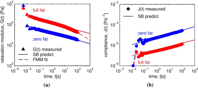
In Fig. 3 we use the quasi-property, G, and fractional exponent, β, obtained from fre-quency sweeps, to predict a priori the relaxation modulus (G(t), Fig. 3(a)) and creep com-pliance (J(t), Fig. 3(b)) of zero-fat and full-fat cheese. We compare the predictions against direct measurements of these linear viscoelastic material functions. Fig. 3(b) shows that at t ≈10−2s creep measurements for both cheese first superpose and then exhibit highly damped
oscillations until the ultimate power-law regime is reached at t ≈ 10−1s. This characteristic short time response is due to a coupling between the complex modulus of the material with the moment of inertia of the rheometer and is often referred to as ‘creep ringing’. It has been extensively studied by Jaishankar and McKinley (2013) for the Fractional Maxwell Model, resulting in a higher-order fractional differential equation that predicts the damped response of power-law materials in the ringing regime at short times as well as at longer times (for
10−3 10−2 10−1 100 101 102 103 103 104 105 106 time, t[s]
ralaxation modulus, G(t) [Pa]
full fat zero fat G(t) measured SB predict FMM fit 10−3 10−2 10−1 100 101 102 103 10−6 10−5 10−4 10−3 time, t[s] compliance, J(t) [Pa −1 ] zero fat full fat J(t) measured SB predict (a) (b)
Figure 3: Measurement and prediction of (a) relaxation modulus G(t) and (b) creep Compliance J(t) of zero-fat (blue) and full-fat (red) cheese at a temperature T=10◦C and for a water/protein ratio w/p = 1.8. (a,b) Zero-fat
cheese shows single power-law behavior up to times t= 100 s of relaxation or creep. (a) Full-fat cheese starts to deviate from a single power-law response after times t= 10 s of stress relaxation. The second power-law relaxation process is captured with a fit of the Fractional Maxwell Model of the relaxation modulus (dashed line).
brevity a corresponding analysis is not included here). Similar ‘ringing’ for the measure-ments of the relaxation modulus G(t) at times t < 10−1s, can be seen in Fig. 3(a). Additional contributions to the high values of G(t) measured at times t < 10−1s, are the Rouse modes of
the biopolymer network (Ng and McKinley, 2008). However this should give an initial slope of d(log(G(t)))/d(log(t))= −0.5 (Bagley and Torvik, 1983), which is not the case here.
To predict the relaxation modulus from the material parameters G and β, we need an
analytical expression for G(t). This is obtained by substituting the step-strain deformation in the constitutive equation for the springpot (Eq. (A.1)) and taking the Laplace transform to solve for G(t)= σ(t)/γ0. Inverse transforming the result gives (Jaishankar and McKinley,
2013):
G(t)= Gt
−β
Γ(1 − β) (6)
whereΓ(z) is the Gamma function (Abramowitz and Stegun, 1964). The predictions of this
two-parameter Scott Blair model (SB) are plotted as solid lines in Fig. 3(a). We see that for zero-fat cheese, both the magnitude and the slope of G(t) are correctly predicted by Eq. (6).
For full-fat cheese, the SB model (fitted to frequency data over the range ω ≥ 0.5 rad s−1)
gives good predictions at times t . 2π/ωmin = 12 s. For times t & 12 s, a second
power-law relaxation process with a steeper slope dominates the dynamics. This can be quantified by adding an additional springpot in series with the first Scott Blair element, which leads to the constitutive equation for the Fractional Maxwell Model (or FMM,Eq. (A.2)). Following the same procedure as that followed for constructing the Scott Blair model, we arrive at an expression for the relaxation modulus of the FMM (Friedrich et al., 1999; Jaishankar and McKinley, 2013):
G(t)= Gt−βEα−β,1−β −G
Vt
α−β! (7)
where Ea,b(z) is the generalized Mittag-Leffler function defined as (Podlubny, 1999)
Ea,b(z)= ∞ X k=0 zk Γ(ak + b), (a > 0, b > 0) (8)
By using the definition for the characteristic time constant in Eq. (A.13), the (dimensionless) argument of the Mittag-Leffler function in Eq. (7) is recognized to be z = −(t/τc)α−β. where
τc is the characteristic time-scale of the Fractional Maxwell model (Eq. (A.13), Faber et al.
(2015)). When we fit Eq. (7) to the full-fat cheese measurements shown in Fig. 3(a), we obtain the dashed line. The second Scott Blair element has a fractional exponent α= 0.65 and is more viscous in character than the first element, which has an exponent β= 0.14. We can check whether the obtained fit values represent true material properties by seeing how they independently predict the storage and loss modulus {G0(ω),G00(ω)} of the same cheese material, by substituting the four model parameters {G,V,α,β} into the expression for G0(ω)
and G00(ω) predicted by the Fractional Maxwell model. This model is obtained by taking the Fourier transform of Eq. (A.2) which gives (Jaishankar and McKinley, 2013):
G∗(ω)= V(iω)
α·G(iω)β
G(iω)α+ V(iω)β (9)
charac-teristic time scale τc from Eq. (A.13), we obtain G0(ω)= G0 (ωτc)αcos(πα/2)+ (ωτc)2α−βcos(πβ/2) (ωτc)2(α−β)+ 2(ωτc)α−βcos(π(α − β)/2)+ 1 (10) and G00(ω)= G0 (ωτc)αsin(πα/2)+ (ωτc)2α−βsin(πβ/2) (ωτc)2(α−β)+ 2(ωτc)α−βcos(π(α − β)/2)+ 1 (11) where G0 ≡ Vτ−αc sets the scale of the stress in the material. The model predictions for the
storage and loss modulus from the FMM are plotted as dashed lines in Fig. 2(b). This shows that frequency domain predictions of this four-parameter model are still consistent with the data available. The second relaxation mode withV = 4.7 × 10⁶ Pa sα and α= 0.65 predicts
a more rapid roll-off in the viscoelastic moduli at low frequencies (ω τc) or long times
(t τc), consistent with the evolution in the stress relaxation modulus G(t) observed in
Fig. 3(a).
In contrast to the Scott Blair model, the Fractional Maxwell Model can predict a cross-over frequency ωc at which G0(ω)=G00(ω), depending on the values of α and β. This
cross-over frequency is sometimes (incorrectly) referred to as a gelation criterion, but marks a transition from viscously-dominated regime (ω ≤ ωc) to elastically-dominated (ω ≥ ωc).
This cross-over frequency can be calculated by equating Eq. (10) and (11) resulting in the following expression ωc = G V " sin(πα/2) − cos(πα/2) cos(πβ/2) − cos(πβ/2) #!α−β1 = τ1 c " sin(πα/2) − cos(πα/2) cos(πβ/2) − cos(πβ/2) #α−β1 (12)
and is real-valued provided 0 ≤ β < 0.5 < α ≤ 1 (as is always obtained for the cheese samples studied here). For the full-fat cheese shown in Fig. 2(b), substitution of the values for the quasi-properties and fractional exponents gives a value for the cross-over frequency of ωc = 1 × 10⁻⁴rad s−1. For cases where the system is predominantly elastic (0 ≤ β < α < 0.5)
or viscous (0.5 ≤ β < α ≤ 1) over the entire frequency domain, no characteristic cross-over frequency exists.
for G(t) are repeated, but now with a step shear stress σ(t)= σ0H(t) as the input and solving
for the resulting strain γ(t). For the Scott Blair model this gives the following expression for the compliance (Jaishankar and McKinley, 2013):
J(t) ≡ γ(t) σ0 = 1 V tα Γ(1 + α) (13)
and for the fractional Maxwell model
J(t)= 1 V tα Γ(1 + α) + 1 G tβ Γ(1 + β) ! (14)
In Fig. 3(b) we plot the measured and predicted creep compliance J(t) for zero-fat and full-fat cheese at 10◦C. The SB model correctly predicts the measured creep compliance in both the zero-fat and full-fat samples from the material parameters obtained independently from the frequency sweep. Extending the SB model to a Fractional Maxwell Model is not required here because the data does not extend beyond tmax' 102s.
From the data shown in Fig. 2 and 3 we have demonstrated that cheese, a fat-filled casein gel, displays power-law relaxation behaviour over a range of temperatures and compositions. The fractional constitutive framework allows us to predict the response of the cheese samples to standard shearing deformations. The wide range of microstructural scales in the material result in a very broad spectrum of relaxation timescales. These can compactly be represented in terms of a power-law relaxation spectrum or a Scott Blair element, and it is necessary to de-termine just two constitutive parameters to make the predictions. These material parameters are obtained by fitting the appropriate fractional expression for the standard linear viscoelas-tic material functions to the measured data. In Part I of this work we have additionally shown how this fractional constitutive framework can be used to derive equations for the texture attributes of firmness (F), springiness (S ) and rubberiness (R). These equations are uniquely expressed in terms of the quasi-propertyG, and the fractional exponent β of the Scott Blair element and for completeness summarized here in Table A.1.
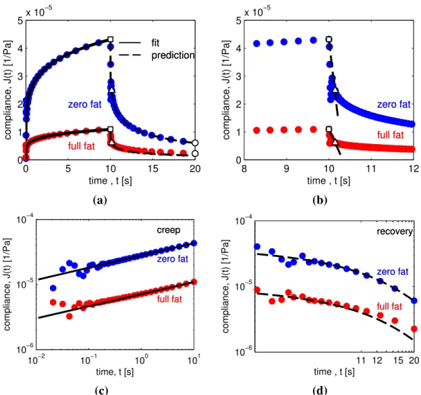
0 5 10 15 20 0 1 2 3 4 5x 10 −5 time , t [s] compliance, J(t) [1/Pa] zero fat full fat fit prediction zero fat full fat fit prediction 8 9 10 11 12 0 1 2 3 4 5x 10 −5 time , t [s] compliance, J(t) [1/Pa] zero fat full fat zero fat full fat (a) (b) 10−2 10−1 100 101 10−6 10−5 10−4 time, t [s] compliance, J(t) [1/Pa] creep zero fat full fat creep zero fat full fat 11 12 15 20 10−6 10−5 10−4 time , t [s] compliance, J(t) [1/Pa] recovery zero fat full fat recovery zero fat full fat (c) (d)
Figure 4: (a) Creep/ recovery experiment (σ0 = 100 Pa) of zero-fat and full-fat cheese at T =10◦C. Dashed
line: prediction of the compliance J(t) in the recovery phase using the Scott Blair element, Eq. (A.11), with tf = 10 s. The material parameters G and β are obtained by fitting Eq. (13) to the compliance J(t) of the
creep phase. The fit result is indicated by the solid line and denoted as “SB fit”. The hollow symbols are the specific points from the creep/ recovery curve which are used to calculate the measured firmness F, (square), springiness S , (triangle), and rubberiness R, (circle). (b) Same experiment as in (a) now plotted over a limited time range −2 < ∆t = t − tf < 2, The absolute slope of the secant (dashed line) represents the springiness
and is calculated with Eq. (A.18). (c,d) Same experiment as in (a) plotted on a log-log scale and with the creep phase (c) and the recovery phase (d) separated. Both phases show some ‘creep ringing’ due to coupling of the elasticity and the moment of inertia of the instrument. (d) The compliance ultimately approaches zero. For full-fat cheese, the Scott Blair model overestimates the recovery, an irreversible flow event appears to have occurred, see section 3.3. These plots demonstrate that our equations correctly predict the firmness, springiness, and rubberiness of power-law materials such as cheese, from the two constitutive material parametersG and β describing the material.
3.2. Fractional equations for firmness, springiness, and rubberiness (FSR)
In section 3.1, we presented the fractional expression for the creep compliance J(t) (Eq. (A.9)) and showed that we can use this equation to obtain the material parametersG and β for a given cheese. Our FSR-equations consist of only these material parameters and a specification of the time of measurement. This suggests that we can also determine values for both springi-ness and rubberispringi-ness by performing a measurement of the compliance J(t); as long as we stay within the linear viscoelastic region; a separate recovery measurement is not required, although in principle it is easy to perform as a second step of an automated sequence im-mediately after a creep loading. Fig. 4 shows that this is indeed the case. The solid lines in Fig. 4(a) and (c) are fits of Eq. (13), the dashed lines in figures Fig. 4(a) and (d) are pre-dictions from Eq. (A.11). Fig. 4(a) shows that we correctly predict the rubberiness (circles) of the zero-fat and full-fat cheese, the latter being the most rubbery. In Fig. 4(b) we have plotted the same experiment as in 4(a) but now we zoom in on the region over which we measure springiness just after the time tf. The secant lines plotted in Fig. 4(b) are predictions
from Eq. (A.18) and show that the zero-fat cheese is the springiest (with the largest rate of recovery), which can be ascribed to its smaller value of the quasi-propertyG.
The equations for firmness, springiness, and rubberiness assume a viscoelastic response that can be described with a single springpot or Scott Blair element. These expressions contain only two material parameters, the quasi-property G and the fractional exponent β, and therefore we call these expressions (Eqs. (A.15),(A.18),(A.21)) the two-parameter FSR-equations. In section 3.1 we have seen that for longer test durations, the addition of a second springpot in series (capturing a separate spectrum of relaxation processes) might be required for a more accurate fit or prediction. Following the same procedure as outlined above, but using the constitutive equation for the Fractional Maxwell Model (FMM) given in Eq. (A.2), we can derive four-parameter formulations of the FSR-equations. The firmness is calculated by taking the inverse of the predicted compliance J(t) of the FMM model Eq. (14), and sub-stituting the fitted material parameters and chosen time of observation, tf. To evaluate the
Maxwell Model, which is given by (Jaishankar and McKinley, 2014): J(t)= t β− (t − t f)β GΓ(1 + β) + tα− (t − tf)α VΓ(1 + α) , for t > tf (15)
Substituting the appropriate times of observation and using the mathematical definitions for springiness Eq. (A.17), and rubberiness Eq. (A.20), gives numerical values for these at-tributes, Eq. (A.23) and Eq. (A.27) respectively. The response for recovery times∆t>>tf is
dominated by the more viscous element and can be approximated by (Jaishankar and McKin-ley, 2014): J(t) ≈ t α f VΓ(α) t tf !α−1 (16) 3.3. Stress-time and flow
We have argued that determining the creep/ recovery curve, introduced to food rheology by Davis (1937), should be the standard rheological test protocol for defining and measuring the firmness, springiness, and rubberiness of food gels. The shape of the curve (and thus the magnitude of F, S and R) is determined by the intrinsic material properties of the test mate-rial, as well as the severity of the creep loading. The latter is determined by setting both the magnitude (σ0) as well as the duration (tf) of the shear stress applied. Davis (1937) denoted
the combination chosen as the ‘stress-time’, with units of Pa s. He showed that setting a high or low stress-time had significant effects on the amount of irreversible flow measured in the material, and thus on the measured food properties. In this section we demonstrate that the FSR-equations correctly predict the magnitude of F, S and R, irrespective of the ‘stress-time’ conditions chosen.
First we look at zero-fat cheese and the linear viscoelastic responses. We have defined compliance-based expressions for the firmness, springiness, and rubberiness of food gels, thus in the linear viscoelastic regime F, S and R are independent of the stress applied. Davis (1937), however, based his conclusions on the flowing properties of cheese on stress-strain curves. To show how the magnitude of F, S and R vary if we were to take the same approach we also examine the effect of stress-time on the magnitude of strain-based definitions of the
three texture attributes. We denote these alternate measures as ˆF, ˆS and ˆRrespectively. Using such strain-based equations is equivalent to assessing F, S and R based on observations by vision only (Bourne (2002); Ewoldt (2013), see Fig. 1(a) in Faber et al. (2015)), without any (tactile) feedback of the stress applied.
The concept of stress-time has recently received a lot of attention in soft matter science, specifically in the study of yielding, where a progressive collapse of the internal structure gives rise to flow. The interplay of stress and time has been used to introduce concepts such as ‘delayed yielding’ (Sprakel et al., 2011) and ‘time-stress superposition’ (TSS) (Gobeaux et al., 2010). However, these two concepts have been applied in the polymer and plastics community for several decades (Matz et al., 1972) and predictive constitutive models have been successfully built on the basis of TSS (Engels et al., 2012).
To illustrate the concept and the consequences, we compare the firmness, springiness, and rubberiness of full-fat cheese at two stress-time conditions, one of which leads to yielding and irreversible flow. In the latter case our equations for F, S and R still correctly predict the measured value of firmness, springiness, and rubberiness. The three curves shown in Fig. 5(a) are creep/ recovery measurements on zero-fat cheese performed at three increasing levels of stress-time. The three cases are: 1) a firmness measuring time tf = 10 s at a stress amplitude
of σ0= 100 Pa; 2) a measurement time of 100 seconds combined with 100 Pa; 3) 100 seconds
at a stress level of 1000 Pa. The times are chosen such that tf1 = tf2/10 = tf3/10, and the
stresses such that σ0,1 = σ0,2 = σ0,3/10. Note that we have taken identical creep and recovery
times within each experiment, thus the time for measuring rubberiness∆tr = tf. In Fig. 5(b)
we have converted the raw strain γ(t) measured for each case to the creep compliance J(t), by dividing each case with the corresponding stress amplitudes. In Fig. 5(c) and (d) we separate the creep compliance from the recovery phase and plot both phases on a log-log scale, to reveal the presence of power-law creep. In Fig. 5(e)-(h) the zero-fat cheese (blue symbols) is replaced by full-fat cheese (red symbols).
Curve 2 and curve 3 in Fig. 5(c) show identical compliances at the end of the curves. We thus measure the same firmness for stress-time conditions 2 and 3 and we have F2 = F3
(a) 0 50 100 150 200 0 0.05 0.1 0.15 0.2 0.25 0.3 0.35 3 time , t [s] strain, γ [−] 2 1 0 50 100 150 200 0 0.05 0.1 0.15 0.2 0.25 0.3 0.35 3 time , t [s] strain, γ [−] 2 1 (e) (b) 0 50 100 150 200 0 0.5 1 1.5 2 2.5 3 3.5 4x 10 −4 3 2 1 time , t [s] compliance, J(t) [1/Pa] 1/firmness springiness 1/rubberiness 0 50 100 150 200 0 0.5 1 1.5 2 2.5 3 3.5 4x 10 −4 3 2 1 time , t [s] compliance, J(t) [1/Pa] 1: σ0 = 100 Pa 2: σ 0 = 100 Pa 3: σ 0 = 1000 Pa (f) (c) 10−2 100 102 10−6 10−5 10−4 10−3 3 2 1 3 2 1 time , t [s] compliance, J(t) [1/Pa] creep 10−2 100 102 10−6 10−5 10−4 10−3 3 2 1 3 2 1 time , t [s] compliance, J(t) [1/Pa] creep (g) (d) 10−2 100 102 10−6 10−5 10−4 10−3 3 time of recovery, ∆ t [s] compliance, J(t) [1/Pa] 2 1 3 2 1 recovery SB prediction FMM prediction 10−2 100 102 10−6 10−5 10−4 10−3 3 time of recovery, ∆ t [s] compliance, J(t) [1/Pa] 2 1 3 1 recovery (h)
Figure 5: Creep/ recovery experiments of zero-fat (blue) and full-fat cheese (red) at 25◦C for three combinations of stress and time. The hollow symbols indicate the points on the creep/ recovery curve that are used to calculate firmness (square), springiness (triangle) and rubberiness (circle). The numbers ’1’, ’2’ and ’3’ correspond to the order of severity of the stress-time loading. (a),(e) Strains γ(t), (b),(f) converted to creep compliances J(t). (c),(g) Same creep curves as in (b),(f) plotted on a log-log scale. (c),(g) Same recovery curves as in (b),(f) plotted on a log-log scale. (c) For zero-fat cheese all the curves coincide and the elastic recovery shown in (d) is well predicted with the Scott Blair model (single springpot). For full-fat cheese (g) enhanced flow sets in when a very high ‘stress-time’ is applied as shown in curve 3. This leads to poor fits (g) and poor predictions (h) of the simple SB element (continuous lines), the Fractional Maxwell Model (dashed lines) gives good fits
though σ0,2 , σ0,3, since in the linear viscoelastic region, firmness is independent of the
stress, and both the test temperature and test time are identical (tf2 = tf3). Our definition of
firmness, Eq. (A.15), and the fractional expression for the compliance, Eq. (13), allow us to calculate any point on the creep compliance curve with the expression:
J(t)= 1 F2 t tf2 !β for t < tf (17)
When we substitute tf1 in Eq. (17) and take F1 = 1/J(tf1), we can correlate the firmness for
the three stress-time cases as:
tf2
tf1
!β
F1 = F2 = F3 (18)
For β= 0.26 and tf2/tf1 = 10, this gives a firmness F1that is 1.8 times smaller than F2 and
F3, which corresponds to what is shown in Fig. 5(b). Such an effect of the stress-time loading
on firmness is in line with Scott Blair’s findings: only the time taken to load a material affects the judgement of firmness, variations in the stress applied have no effect (Scott Blair et al., 1947), at least within the material’s linear regime. The magnitude of these temporal effects are determined by the scaling factor in Eq. (18), and the fractional exponent β. For a purely elastic material with β= 0, this time effect is zero, for a purely viscous material, with β = 1 the time effect is equal to tf2/tf1. If we defined firmness as the inverse of the strain at the end
of creep and called it ˆFthan we would get: tf3 tf1 !βσ 0,3 σ0,1 ˆ F1 = σ0,3 σ0,1 ˆ F2 = ˆF3 (19)
For zero-fat cheese values in this experiment we have 18 ˆF1 = 10 ˆF2 = ˆF3which corresponds
to the relative vertical position of the maximal strains γ in Fig. 5(a).
Springiness can be graphically distinguished in the curves of the creep compliance, Fig. 5(b), as the distance between the values of the measured compliance at tf, and tf+ ∆ts
(corre-sponding to the squares and the triangle respectively). Visually, it appears to be equal for all three stress-time conditions, so neither time nor stress has a significant effect on springi-ness. Numerical values of the springiness from the data in Fig. 5(b), give S1 = 3.5 × 10⁻⁴,
S2 = 4.6 × 10⁻⁴, S3 = 4.3 × 10⁻⁴(Pa s)−1so variations are less then 25 %.
This is what we predicted from Eq. (A.18): at short times in the recovery phase (∆ts= 0.1
s), springiness is only a function of the fractional exponent β and the quasi-propertyG. So for the three cases, the springiness can be calculated from the expression:
S1= S2 = S3 = −10−1(β−1) GΓ(1 + β) (20)
If we defined springiness from measured deformations instead of compliances, we would have obtained: ˆ S1 = ˆS2= σ0,3 σ0,1 ˆ S3 (21)
This is what we observe in Fig. 5(a), the vertical distance between the square and the triangle is 10 times larger for curve 3 than for curve 2.
In part I of this work we demonstrated that the rubberiness R, Eq. (A.21), depends on
two times, the creep time tf elapsed before measuring the firmness during creep and the
subsequent elapsed time∆tr= tr− tf taken to measure rubberiness during recovery. In our
stress-time experiments we have chosen tf to be equal to∆tr(this is true for all three curves
for each cheese shown in Fig. 5. Substituting this in Eq. (A.21)) gives
R1 = R2 = R3 = 2 − 2β (22)
We have defined rubberiness from a ratio of two compliances as R= 1− J(tf + ∆tr)/J(tf).
Converting this into a definition based on a ratio of two strains, ˆR = 1 − γ(tf + ∆tr)/γ(tf),
requires both compliances to be multiplied by the same stress σ0, which therefore cancels
out. Thus R= ˆR.
For the firmness, springiness, and rubberiness of full-fat cheese we follow the same anal-ysis as for the zero-fat cheese sample. The curves 1 and 2 in Fig. 5(e) and (f) show that for stress-time cases 1 and 2, equations (18)-(22) apply. However for stress-time case 3, with a long test time tf = 100s at a large stress of σ0 = 1000 Pa, the creep response of curve 3 in
stress-loadings, the two-parameter Scott Blair model for the creep compliance J(t) is insufficient to describe the full range of retardation processes in the material, and the material begins to flow irreversibly at long times. To describe this flow we fit the data to the functional form predicted by the four-parameter Fractional Maxwell Model, given by Eq. (14) and Eq. (A.10). The dashed line denoted with a ‘3’ in Fig. 5(g) shows that this gives a greatly improved fit at large stress-times. This also leads to good prediction of the recovery data, as demonstrated by the dashed line labeled ‘3’ in Fig. 5(h). We emphasize here again that this prediction is obtained by substituting a priori fitted material parameters for the FMM model into the corresponding expression for the recovery phase, Eq. (15). The more elastic element has a quasi-property value ofG = 0.4 × 10⁵Pa sβ and a fractional exponent β= 0.13. The second
element is a viscous dashpot: V = 7.6 × 10⁵ Pa sα and α = 1 (see Table A.2). One can
say that the first element describes the semi-solid, fractional viscoelastic nature of cheese, whereas the second element (which dominates at long times) represents the ultimate transi-tion of the fat-filled material at large values of the stress-time to a liquid with a very high viscosity.
The stress-induced yielding and failure of casein gels has recently been studied in detail by Leocmach et al. (2014), who combined creep experiments with ultrasonic velocimetry imaging. They showed that at large strains, casein gels display brittle-like failure which is a resultant of two consecutive physical processes. The first is reversible primary creep, also referred to as Andrade creep (Andrade, 1910). In contrast to crystalline or amorphous solids, the strain in viscoelastic gels can be fully recovered during primary creep (Leocmach et al., 2014), which agrees with the prediction of the SB element. The second process is nucleation and growth of fractures, leading to plastic deformation and eventually complete sample failure. This regime is commonly called tertiary creep. In between lies a transition regime which is denoted as secondary creep.
If we map these processes onto our measurements and model predictions, we can
con-clude that the more elastic SB element in the FMM model (with parametersG and β)
repre-sents, in compact form, the spectrum of reversible viscoelastic processes in the material, and the second element in series (with parametersV and α) models empirically any additional
ir-reversible plastic part. By arranging the elements in series we additively combine the elastic and plastic strains that result from each physical process. When fitting the FMM to rheo-metric creep data obtained at large stress-times (which may contain a yielding event) we are using a model derived from linear viscoelastic theory to capture a non-linear viscoelastoplas-tic response. It is important to recognize that a linear model such as the Fractional Maxwell Model does not predict a yield stress or strain, this requires more sophisticated non-linear models that include a damping function (Jaishankar and McKinley, 2014) or a damage func-tion (Tanner et al., 2008; Mohammed et al., 2013). However, fitting creep data at small and moderate strains to the FMM enables us to effectively predict the recovery phase of the bulk material very well (compare the five curves in Fig. 5(d) and (h)), suggesting that it also correctly describes two of the primary processes occurring during the initial loading and unloading phases. We will use this feature to our advantage to separate viscoelastic, recover-able contributions to the firmness, springiness, and rubberiness, from the additional plastic, non-recoverable contributions that occur in the case of irreversible flow in the material.
We have demonstrated that our definitions for the firmness F, springiness S , and rub-beriness R, of food gels give correct quantitative predictions of the effect of the stress-time loading on measurements of F, S , and R. If the deformation amplitude remains within the linear viscoelastic regime, then the magnitude of the springiness is not affected by stress or time. For our chosen times of observations for the firmness and rubberiness such that tf=∆tr,
the texture attribute of rubberiness R, becomes stress- and time-independent as well. When very large stress-time loading leads to larger deformations in the viscoelastoplastic region, i.e. resulting in strains in the material that are larger then the yield strain, our four-parameter FSR-equations derived from the Fractional Maxwell Model (FMM) correctly predict the variation in the firmness, springiness, and rubberiness of cheese, provided that the material has not en-tered the regime of tertiary creep and fracture. The presence or absence of an irreversible flow event at large values of the stress-time, has a large impact on quantitative rheological mea-surement of the firmness, springiness, and rubberiness of food gels. This suggests that when the firmness, springiness, and rubberiness of a food gel is evaluated by hand, the magnitude of the stress-time loading applied should be defined as precisely as possible, conforming to
zero fat low fat full fat 10°C 30°C 30°C filled open open 1.5 1.8 2.1 2.4 2.7 103 104 105 106 firmness, F [Pa] water / protein [g/g] ‘firm’ ‘soft’ 1.5 1.8 2.1 2.4 2.7 10−6 10−5 10−4 10−3 springiness, S [1 /(Pa s)] water / protein [g/g] ‘springy’ ‘squishy’ 1.5 1.8 2.1 2.4 2.7 0.7 0.8 0.9 1 rubberiness, R [Pa] water / protein [g/g] ‘rubbery’ ‘moldable’
(a) Firmness (b) Springiness (c) Rubberiness.
Figure 6: Composition-temperature-texture plots of Gouda cheese. (a) firmness F, (b) springiness S , (c) rub-beriness R. The plots are obtained by determining the quasi-propertyG, and the fractional exponent β, from forty frequency sweeps, and entering the value in the FSR-equations. The time of observations for firmness and rubberiness are tf= ∆tr= 10 s. For springiness ∆ts= 0.1 s. (a) Cheese is most firm at low temperature, and at a
low water/ protein ratio, and high fat content. (b) Springiness is inversely related to firmness, the softest cheese is the most springy. (c) Rubberiness is a function of the fractional exponent only.
3.4. Comparing cheese formulations on the basis of firmness, springiness, and rubberiness In Fig. 2 we showed four representative frequency sweeps of Gouda cheese, varying in temperature and composition. In all cases the cheese showed a clear power-law relaxation. This relaxation behaviour can be adequately described by the Scott Blair model for the com-plex modulus, Eq. (2). By fitting this model to the dataset, we determine the numerical values of the two material properties that characterize this cheese: the quasi-propertyG and the frac-tional exponent β. From these material parameters we can calculate firmness F, springiness S, and rubberiness R, at any time of observation, using equations (A.15), (A.18) and (A.21).
We demonstrate the power of these FSR-equations in Fig. 6. In total we have measured 40 combinations of cheese composition and temperature, corresponding to 80 curves of the frequency-dependent storage and loss modulus, G0(ω) and G00(ω). We condense this exten-sive dataset into the three composition-temperature-texture plots of the firmness, springiness, and rubberiness, shown in Fig. 6. The definitions for FSR, in equations (A.15), (A.18) and (A.21) allow us to enter any time of observation of interest; here we select tf= ∆tr= 10 s for
Compositional changes are represented in two ways. On the abscissa we have plotted the water/protein ratio (w/p) of the cheese. Variations in fat content are represented by the three colors, blue, green and red, for zero, low and full-fat respectively. Since the material prop-erties of many food products are highly temperature sensitive (Szczesniak, 1975), we have measured the viscoelastic properties of the cheese at T = 10◦C (filled markers), a temperature
relevant for storing cheese, and also at T = 30◦C (unfilled markers), a temperature the cheese will attain during oral processing.
We interpret the data in this figure as describing the reformulation window for firmness. Under storage conditions the cheese has to be firm; this inhibits sagging and gives optimal slicing properties. Our reference point for optimal firmness prior to consumption is full-fat cheese at T = 10◦C, having its standard water/protein ratio of w/p =1.8. This appears
to be the most firm cheese. Now the challenge for the food engineer dealing with product reformulation becomes apparent: at T = 10◦C either a reduction of fat content, or an increase
of water content, will always lead to a softer cheese. This will inevitably lead to inferior processing properties. When removing fat from the product for reasons of calorie reduction, one has to lower the water/protein ratio as a countermeasure to retain firmness.
When increasing temperature we see that our reference full-fat cheese shows a pro-nounced drop in firmness. It can be argued that this ‘thermal-induced softening’ gives rise to a melting sensation during consumption (Devezeaux de Lavergne et al., 2015). This further augments the ‘stress-induced softening’ we observed in Fig. 5(g). Removing fat significantly reduces this thermal softening-effect on cheese firmness. Changing the water/protein ratio has no effect on the temperature-firmness relation.
The strong ‘thermal-induced softening’ of full-fat, semi-hard cheese can be physically explained using filled gel models to describe the structure shown in Fig. 1(d). Yang et al. (2011) fitted a variety of these models to data for the storage modulus G0(ω) of Cheddar
cheese, at a frequency ω= 1 rad s−1. Depending on the model applied, they predicted that
at T = 10 ◦C, the shear modulus, G
f, of the filler (fat) is 6-11 times larger than the shear
modulus of the matrix Gm. At T = 10◦C the filler thus acts as a firmness enhancer. When
decrease of the filler modulus Gf by a factor ranging from 10-27, depending on the model
applied. Over the same temperature range, Gmdecreased not more than a factor of two, which
corresponds to what we measure for the decrease of the storage modulus of zero fat cheese
when raising the measuring temperature from T = 10 ◦C to T = 30 ◦C (Fig. 2(a) and (c),
blue filled symbols). At T = 25 ◦C, Yang et al. (2011) measure a storage modulus, G0(ω),
that is independent of the fat content of the cheese, which is similar to what we find for the firmness F, at T = 30◦C and a time of observation t
f= 10 s. (Fig. 6(a), hollow symbols).
Note that the firmness of low-fat cheese (green symbols in Fig. 6(a)), is approximately equal to the firmness of zero-fat cheese (blue symbols) at both temperatures. Apparently there is a threshold value for the fat volume fraction,Φf, below which this cheese constituent has no
significant effect on the overall firmness of the cheese.
Next we examine the effect of temperature and composition of the cheese on the springi-ness S , plotted in Fig. 6(b). We see that the softer cheese will be the most springy, which corresponds to the anti-correlation between firmness and springiness found in panel tests (Goh et al., 2003). The trend can be explained by the inverse relation between springiness and firmness, as expressed in Eq. (A.18), and has also been observed in the Texture Profile Analysis of reformulated muffins (Matos et al., 2014).
The rubberiness plot, Fig. 6(c), shows that S and R indeed are two distinct properties, and they scale differently with composition and temperature. Since we have chosen the time of observation ∆tr for rubberiness to be equal to tf, we can use Eq. (22) to calculate R. This
expression shows that under these time conditions, the rubberiness R is only a function of the fractional exponent β. For our cheeses, the measured values for this exponent range from 0.14 ≤ β ≤ 0.25. Fig. 6(c) shows that for these values the strain recovery is fast; in 10 seconds 80-90 % of the strain is recovered for all samples.
We can conclude that reformulating a cheese by merely changing the relative amount of protein, water and fat will give great firmness deficits, both from a sensory texture as well as a processing perspective. To decouple this texture-composition relation, alternative structuring routes need to be explored. This exploration should start with a physical understanding of the observed scaling between fat content and water/protein ratio on the one hand, and firmness,
rubberiness and springiness on the other. Such understanding requires structure-texture rela-tions such as the filled gel models tested by Yang et al. (2011) or such as the model proposed by Bot et al. (2014), who developed a structural model for the firmness and syneresis of food gels as a function of composition and temperature based on a set of recursive power-law scaling relations. However both Yang et al. (2011) and Bot et al. (2014) do not account for the time-dependence of the magnitude of the firmness F, and the structure-texture relations they use have not been extrapolated to other texture attributes assessed at first touch and first bite. Since we have shown that the attributes F, S and R, all stem from the quasi-property, G, and the fractional exponent β of the viscoelastic test material, a coupling of the models discussed by Bot et al. (2014) and Yang et al. (2011) to the magnitudes of the quasi-property G, and fractional exponent β of Scott Blair’s springpot, would be the next step to take in the development of an appropriate structure-texture model.
3.5. Practical relevance of firmness measurements
In section 3.4 we demonstrated the use of the FSR-equations as a screening tool for texture optimisation. In Fig. 6 a wide range of formulations are plotted in texture-composition-temperature space. The three plots show at a glance the reformulation window for cheese with respect to the firmness, springiness, and rubberiness. However the construction of these plots requires a substantial experimental effort, while a structure-texture model should reduce these efforts and point a priori towards the most optimal formulation and structure.
We have chosen to measure firmness, springiness, and rubberinessusing a stress-controlled experimental protocol. Such an experiment exposes temporal effects in the material more di-rectly than the more common rate-controlled compression experiment used in Texture Profile Analysis (Friedman et al., 1963). Moreover, it enables us to interconnect the firmness F, to situations where stresses are applied for short times, such as sensory texture measurement, or for long times, such as in storing cheese (Fig. 1(a) in Part I, Faber et al. (2015)). We have developed rheological definitions of firmness, springiness, and rubberiness based on an understanding of compliances, since in the linear viscoelastic regime, the judgement of firm-ness is independent of the stress applied (Scott Blair and Coppen, 1942a). To extrapolate
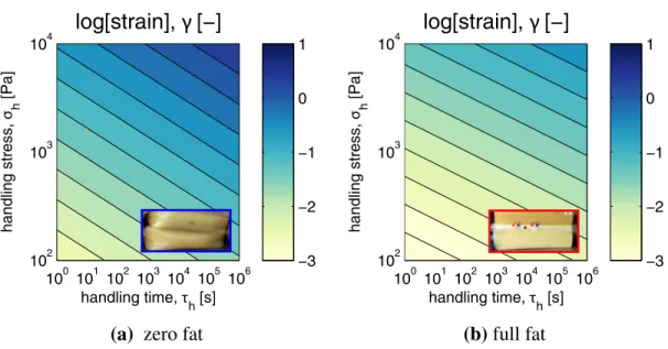
100 101 102 103 104 105 106 102 103 104 handling time, τh [s] handling stress, σ h [Pa]
log[strain], γ [−]
−3 −2 −1 0 1 100 101 102 103 104 105 106 102 103 104 handling time, τh [s] handling stress, σ h [Pa]log[strain], γ [−]
−3 −2 −1 0 1(a) zero fat (b) full fat
Figure 7: The effect of handling stress, σh and handling time τh on the predicted deformation of (a) zero fat
and (b) full-fat cheese at 10◦C. Shear strains, γ are plotted as contours on a log-scale and calculated from Eq. (23). At equal stress-time loadings, the softer zero-fat cheese, (F= 0.2 × 10⁵) Pa generates lighter contours
compared to the firmer full fat cheese, F= 1 × 10⁵Pa, as a result of the higher strains accumulated. The slopes of the contours are equal to the fractional exponent β. For zero-fat cheese, β = 0.18 and for full-fat cheese β = 0.14. At stress-time loadings that lead to irreversible flow, Eq. (23) is not accurate and the predicted strains are under-estimated. Stress-time conditions for texture judgment are located in the top left corner of the plots, where irreversible flow is desired to prevent rubberiness. Stress-time conditions for storing cheese on the shelf are located on the bottom right corner of the plots, where higher levels of firmness favour shape retention.
the measured firmness to how a cheese performs under practical conditions, e.g. whether it will retain its shape when stored on a shelf, we need to convert a firmness measurement to an expected deformation. In section 3.3 we revisited the concept of stress-time, originally introduced by Davis (1937), and we showed how to calculate the resulting material strains γ from the firmness F, for a certain stress-time loading profile. In Fig. 7 we plot the evolu-tion in the sample strain as contours in stress-time space for creep loading of both zero-fat (a) and full-fat (b) cheese at 10◦C. The stress-time space is spanned by the range of typical handling stresses σhand handling times τhcommon in the cheese industry. The contour lines
for specific values of the strain γ(τh, σh) are calculated from the expression
γ = σh F τh tf !β (23) One can obtain insight into the practical relevance and implications of a firmness
mea-surement by considering three terms in this expression. First, we focus on the product σhτ β h
in the numerator, which is the measure of stress-time inherent to the handling process to which the cheese is subjected. When firmness is judged by hand, stresses are high and times are short, which corresponds to the upper left corner of each plot in Fig. 7. When a cheese is stored on the shelf, the imposed stresses (arising solely from body forces) are relatively low, but times can be of the order of weeks. This is represented by the lower right corner of the graph. Under these conditions the full-fat cheese depicted in Fig. 7(b) will be the least deformed, since it is the most firm.
The second term of interest in Eq. (23) is the ratio τh/tf which is a dimensionless ratio of
times in the spirit of Reiner’s original definition of the Deborah number (Reiner, 1964). For cheese subjected to creep loading, the characteristic times in this ratio are the values inherent to the handling process to which the material is subjected and that over which the firmness is determined. For the cheese industry, handling times vary from τh = 1 s (for firmness judged
by hand) to τh= 106− 107s (for storing cheese on a shelf). For a time of observation tf = 10
s this gives a range for τh/tf= 10−1− 106. A high value for τh/tf implies that in the laboratory
the rheologist is probing timescales much smaller than the practical time scale of relevance for the material and one should be careful of extrapolating conclusions from a linear viscoelastic measurement performed over a limited frequency range or a single firmness measurement.
Finally, we learn from Eq. (23) that the deformation of a cheese subjected to creep loading can be factorised in two parts. The first is an instantaneous deformation, observed after a very brief period of stress-time loading. The scale of the instantaneous deformation is set by σh/F. It is worth noting that the instrumental resolution of this instantaneous deformation
is restricted by the response time of the rheometer used. The final deformation caused by the stress-time loading is obtained by multiplying σh/F with the factor (τh/tf)β. For a purely
elastic material, β= 0 and this factor is thus (τh/tf)0 = 1. For such a material, viscoelastic
effects are absent and all contour lines in Fig. 7 are horizontal. For a purely viscous material β = 1 the effect of the elapsed time on strain is linear such that the iso-strain lines have a slope of -1 on this logarithmic plot.
canonical fractional constitutive equation of a single springpot or Scott Blair element (SB). In section 3.1 and 3.3 we have shown that for cases where the stress-time loading leads to a secondary relaxation process in the cheese, we are still able to predict the firmness, springiness, and rubberiness within the fractional constitutive framework. All we require is a generalization of the constitutive model with a second element in series, which yields the equation of the Fractional Maxwell Model, Eq. (A.2). In section 3.3 we have shown that full-fat cheese begins to flow plastically when subjected to high stress-time loadings. This failure may be proceeded by a secondary relaxation processes caused by the propagation of micro fractures in the material (Leocmach et al., 2014). Such microscopic phenomena of course cannot be captured by a bulk phenomenological model such as the FMM, but are captured empirically by the second viscous-like springpot element (with α ≈ 1).
4. Conclusion
The FSR-equations we have developed for a typical power-law food gel contain only two material parameters, the quasi-propertyG(or scale factor) of the gel and the fractional exponent β (Scott Blair, 1947). The resulting stress or strain in the viscoelastic material depends on the experimental time of observation toand the loading protocol. The two material
parameters that characterize the Scott Blair element can be extracted from measurements of any of the standard linear viscoelastic material functions: complex modulus, G∗(ω), storage modulus, G0(ω), loss modulus, G00(ω), relaxation modulus, G(t), or creep compliance, J(t).
When a food gel is subjected to creep loadings, the final deformation of the gel depends on its intrinsic firmness and the severity of the loading. Davis (1937) introduced the concept of ‘stress-time’ to qualitatively discuss the effects of loading severity on cheese deformation. We have demonstrated that our equations for the firmness F, springiness S , and rubberiness R, of food gels give correct quantitative predictions of the effect of the stress-time loading on cheese deformation and the resulting values for F, S and R. If the stress-time loading to which the cheese is subjected will cause the cheese to reach its yield strain during the creep phase, the material will start to behave in a viscoelastoplastic nature and our two-parameter FSR-equations (of Scott Blair type) cannot predict the recovery phase correctly. Four-parameter FSR-equations derived from the Fractional Maxwell Model appear to give much better descriptions of the post-yield, secondary creep response, by incorporating an
irreversible viscous term (with viscosity η = V and α ≈ 1). This approach allows us to
correctly predict the incomplete recovery of the material in the case of irreversible (plastic) flow contributions.
We have presented two methods of using the FSR-equations for product reformulation. The first is to measure the linear viscoelastic response for a wide range of product formu-lations, extract the material parameters G and β of each formulation, and construct three composition texture plots. This reveals the operating window for reformulation when re-quired levels for each texture attribute are available. Our analyses of different cheeses show that fat acts as the perfect filler in modulating firmness, springiness, and rubberiness for