Density of States of Impure Palladium
Deutride/Hydride
by
Irfan Ullah Chaudhary
Submitted to the Department of Electrical Engineering and
Computer Science
in partial fulfillment of the requirements for the degree of
Master of Science in Computer Science and Engineering
at the
MASSACHUSETTS INSTITUTE OF TECHNOLOGY
February 1996
@ Irfan Ullah Chaudhary, MCMXCVI. All rights reserved.
The author hereby grants to MIT permission to reproduce and
distribute publicly paper and electronic copies of this thesis
,
document in whole or in part, and to grant others the right to do so.
,AS.SAC;H IUSETTS INSTITUTE OF TECHNOLOGY
APR 1 1 1996
Author..
ULIBRARIES
A uthor ....
~..
...
.
..- .. .-.... . ...
Depart nent of Electrical Engine ing and Computer Science
/
February, 1996
Certified by..
...
...)Peter
L.
Hagelstein
Associate Professor
Thesis Supervisor
A ccepted by ...
.
...
I
Frederic R. Morgenthaler
Chairman, Departme htal Committee on Graduate Students
Density of States of Impure Palladium Deutride/Hydride
by
Irfan Ullah Chaudhary
Submitted to the Department of Electrical Engineering and Computer Science
on February, 1996, in partial fulfillment of the
requirements for the degree of
Master of Science in Computer Science and Engineering
Abstract
The dynamical matrix method with fixed force constants is used to calculate the
density of states of a palladium deutride/hydride lattice with vacancies. Perturbative
and non-perturbative techniques are used to try and speed up the computation. The
most important computation is the density of states calculation of a perfect palladium
deutride/hydride lattice with one Pd vacancy. It is found that the vacancy modes
pile up near the bottom of the optical band.
Thesis Supervisor: Peter L. Hagelstein
Title: Associate Professor
Acknowledgments
MIT has been a bittersweet and strange experience. In retrospective, I think, the
human experience (however little!!) has a much more lasting impression than the
technical knowledge gained. Peter has been a source of inspiration. He is the perfect
example of how an "ideal" professor should be in an ideal world (unfortunately the
world is somewhat non-ideal!!). Owl and Bird have been great....Ammee and Abbu
totally amazing. Without Idol's sarcasm, life wouldn't have been as much "fun". Asad
helped me a lot with the technical stuff, and I think Sumanth's spirit was somehow
trying to guide me to write bug-free code (although I don't think it succeeded!). He
also wrote a part of the code for the Embedded Atom Method. Jim, (as he has
been for the past 6 years) was a great help, friend and mentor. Anyway the list can
continue, and I have to catch a flight tomorrow in the afternoon...
"I'm out of here...I'm history. No! I'm mythology. Nah! I don't care what I
am. I am free!!!" The Genie in Aladdin.
Contents
1 Introduction
9
1.1
Palladium ...
...
..
12
1.2 Palladium deutride/hydride ...
....
14
2 Theoretical Background
17
2.1
The Dynamical Matrix ...
...
.
17
2.2 Building The Dynamical Matrix ...
..
19
2.3 Speeding up the calculation ...
....
20
2.3.1
Symmetries in the Brillouin zone . ...
20
2.3.2
Non-degenerate Perturbation Theory . ...
25
2.3.3
Degenerate Perturbation Theory . ...
26
2.3.4
Linear Extrapolation ...
.... .
. . . .
.
28
3 Results
3.1
Checks
...
3.1.1
Phonon Spectrum . . . .
3.1.2
Density of states . . . .
3.2 Comparison Of Various Methods
3.3 Dilute Limit .
...
3.4 The Fukai Structure . . . ..
3.5 Vacancy modes near a Pd vacancy
30
.
. . .. .
30
. . . .
.
31
.. . .
.
31
.. . . .
.
32
.. . .
.
35
.. . .
.
38
.. . .
.
38
4.1
Main results ...
...
..
42
4.2
Relaxation ...
. .
.. .
.
44
4.2.1
Embedded Atom Method ...
.
44
4.2.2
Minimization ...
..
. .
...
44
4.2.3
Results ...
....
...
45
4.3 Further Research . . . .
. . . . .
45
A Force Constants For Different Directions
47
B Construction Of The Dynamical Matrix
49
C Detailed Results Of Calculations
52
List of Figures
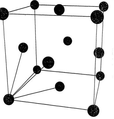
1-1 The top figure shows the palladium lattice. The bottom figure shows
the palladium hydride lattice. ...
13
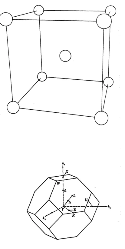
1-2 The top figure shows a bcc lattice. The bottom figure shows the first
Brillouin zone of Pd or PdH ...
15
2-1 The top figure shows the dispersion relation for a cell with lattice
constant ao. The bottom figure shows the same dispersion relation
for a supercell with lattice constant 2ao. .
. . . ...
21
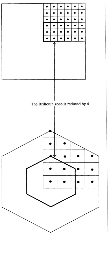
2-2 The figure shows two Brillouin zones. The square BZ does not cause
any problems when scaling down. However the bottom one causes
boundary problems ...
...
23
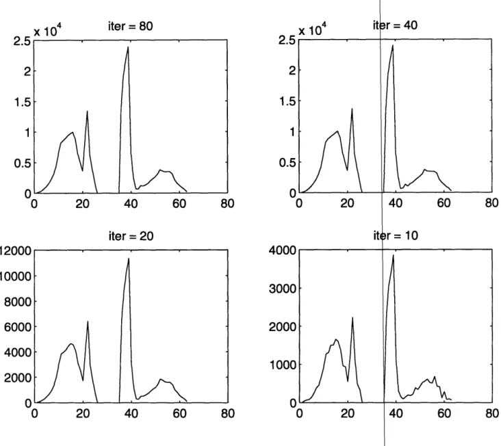
3-1 Density of state for different PdD supercells (in arbitrary units). Top
left is 1 x 1 x 1, top right is 2 x 2 x 2, bottom left is 3 x 3 x 3, bottom
right is 4 x 4 x 4 . . . .
33
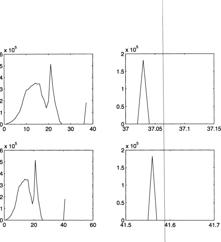
3-2 The top two figures show the density of states for a 3 x 3 x 3 cell with
a deuterium atom added at a,(1, 1, 1/2). The bottom figures show the
density of states when hydrogen atom is added at the same position..
36
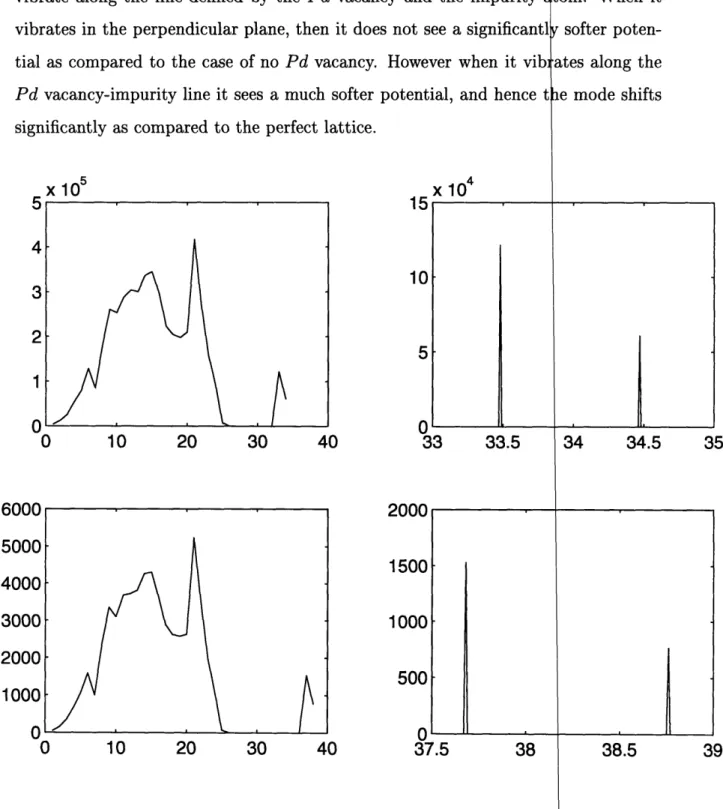
3-3 The top two figures show the density of states for a 3 x 3 x 3 cell with
a deuterium atom added at ao(1, 1, 1/2) and a Pd atom removed from
ao(1, 1, 1). The bottom figures show the density of states for the same
structure with hydrogen replacing the deuterium. . ...
. .
37
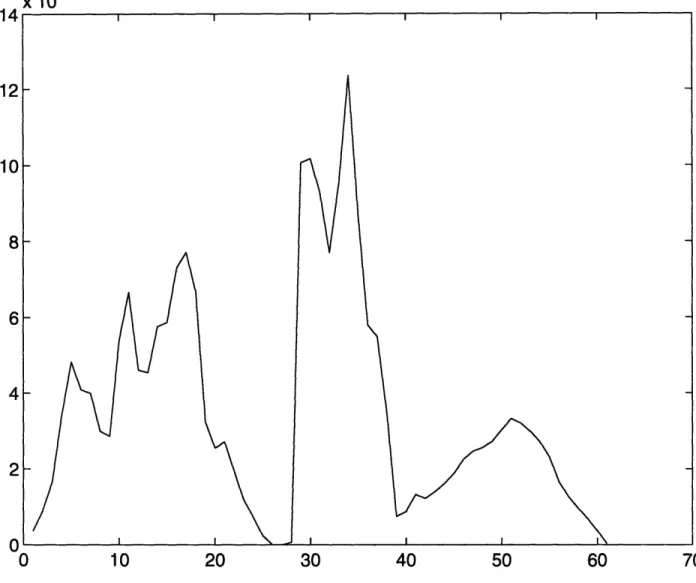
3-4 The figure shows the density of states for the Fukai structure for
3-5 The top figures show the density of states for a perfect Palladium
Deutride lattice. The bottom figure shows the density of states with
Pd at ao(1, 1, 1) missing ...
40
3-6 The top figures show the density of states for a perfect Palladium
Hydride lattice. The bottom figure shows the density of states with
Pd at ao(1, 1, 1) m issing ...
41
B-1 A simple 2 dimensional structure. . ...
.
49
C-1 Cell size is 1 x 1 x 1. No perturbation theory or linear extrapolation
is used . . . .
53
C-2 Cell size is 1 x 1 x 1. The graphs are calculated using non-degenerate
perturbation theory ...
54
C-3 Cell size is 1 x 1 x 1. First 3 graphs are calculated using degenerate
perturbation theory. The last graph is calculated using non-degenerate
perturbation theory with linear extrapolation
. ...
55
C-4 Cell size is 1 x 1 x 1. The graphs are calculated using non-degenerate
perturbation theory with linear extrapolation . ...
56
C-5 Cell size is 1 x 1 x 1. The first graph is calculated using non-degenerate
perturbation theory with linear extrapolation. The last three graphs
use degenerate perturbation theory with linear extrapolation ....
.
57
C-6 Cell size is 2 x 2 x 2. Perturbation theory or linear extrapolation were
not used for the calculation of these graphs . ...
58
C-7 Cell size is 2 x 2 x 2. The first graph is calculated using non-degenerate
perturbation theory, the second with degenerate perturbation theory,
and the last two with non-degenerate perturbation theory with linear
extrapolation ...
59
C-8 Cell size is 3 x 3 x 3. No Perturbation theory or linear extrapolation
is used in the calculation of the first three graphs. The last graph uses
non-degenerate perturbation theory with linear extrapolation ....
.
60
List of Tables
1.1
Relation between size of unit cell and time taken to diagonalize a m x m
matrix(m is the number in column 2) . ...
11
2.1 Force Constants in dyns/cm ...
..
18
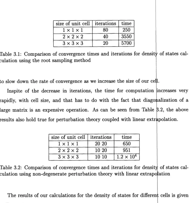
3.1
Comparison of convergence times and iterations for density of states
calculation using the root sampling method . ...
32
3.2
Comparison of convergence times and iterations for density of states
calculation using non-degenerate perturbation theory with linear
ex-trapolation . . ... . . . .
. . . .
32
3.3 comparison of convergence times for different methods ...
34
B.1 The toy force constants ...
50
C.1 Comparison of various methods ...
. . . .
61
C.2 Mistakes for a 1 x 1 x 1 cell ...
62
C.3 Mistakes for a 2 x 2 x 2 cell ...
... ....
62
Chapter 1
Introduction
The calculation of the frequency spectrum of an impure lattice is an old problem. It
was first tackled by Lifshitz in the 1940s[1]. He considered a single impurity atom
in an otherwise perfect lattice 1. Since then many, including Maradudin [3] and
Dawber and Elliot [2] have considered similar such problems. The main results of
their analysis were that:
* the perturbed modes with frequencies in the continuum range were changed
near the defect atom
* when a light impurity atom was introduced into the lattice, localized modes
with frequencies above the range of unperturbed modes appear.
We are specifically interested in a lattice of palladium deutride/hydride. A great
deal of literature is available on this specific lattice [4, 5, 6, 7]. Unfortunately all the
papers have only considered substituting hydrogen with vacancies or other atoms.
This is no coincidence. The reason for such a choice is that when people are doing
experiments they try to load palladium with hydrogen. Ideally PdD/H would have
a NaCi like structure.
2. But hydrogen does not fill all the octahedral sites in the
lattice, and hence it is physically interesting to consider the case of PdDX or PdHx,
where x is any real number between 0 and 1.
'The force constants for an imperfect lattice are assumed to be the same as the ones for a perfect lattice
2
However our interest is in a palladium deutride/hydride structure which has Pd
vacancies. It is interesting physics in its own right, but we are mostly interested in
this structure because it plays an important part in the Coherent Neutron Transfer
Theory [8, 9] put forward by Peter Hagelstein. According to this theory there is a
mechanism through which the lattice and the nucleus can exchange energy. This is
a very startling claim, because solid state and nuclear physicists, both, claim that
such an energy transfer is absolutely impossible. The reason is very simple: nuclear
energy is on the order of MeVs whereas lattice energy is on the order of eVs. In order
for a nucleus to couple to a lattice, 106 phonons need to be destroyed/created. The
probability of such an occurrence is vanishingly small.
But there is another way for a lattice to transfer energy. Let us assume that
there is a large number of phonons,N, in one mode. If through some mechanism,
these phonon modes are shifted by 6w. Then there is a net change in energy of
AE
=
Nh6w
This energy is transfered to the mechanism which caused the change in: the frequency
in the first place.
Palladium is much heavier as compared to deuterium/hydrogen.
3Thus it
oscil-lates at a significantly lower frequency as compared to the deuterium/hydrogen. The
low frequency region is called the "acoustical band" and the high frequency region
corresponding to the oscillating deuterium/hydrogen atom is labeled as the "optical
band". However if we make a palladium vacancy, then the 6 deuterium/hydrogen
atoms surrounding it will vibrate at a lower frequency. And if the frequency is such
that it falls in between the optical and the acoustical modes then the impurity modes
are said to be in the band gap. If this were the case then the 18 phonon modes would
drop down from the optical band to the vacancy impurity band. The excess energy
AE would go into the nuclear process which caused the Pd vacancy to be created in
the first place. So our hope is that when we create a Pd vacancy in the palladium
3
deutride/hydride lattice then we will find the phonon modes in the band gap.
The way we propose to solve our problem is theoretically quite straight forward.
We take a n x n x n super cell of palladium hydride/deutride. From tlis supercell we
remove one or more Pd or D/H atoms. Then using periodic boundary conditions, we
set up the dynamical matrix of this supercell, and diagonalize this matrix to get the
eigenvalues. The numerical details are rather tiresome, but the theory is very well
established. The details can be found in the next chapter and in Appendix B.
But even before doing any calculations, it is obvious that the size! of the matrix
and the diagonalization time increases very rapidly with n, the size of the supercell.
This can be seen from Table 1.1.
4size of unit cell size of matrix
tl
t
21
6
<1
<1
2
48
<1
1
3
162
7
32
4
384
87
415
Table 1.1: Relation between size of unit cell and time taken to diagonalize a m x m
matrix(m is the number in column 2)
To get the density of states calculation to converge, we needed tc form and
di-agonalize this dynamical matrix at approximately 500 points in the $rillouin zone.
Thus the problem becomes rather unmanageable for a 3 x 3 x 3 or a 4 1x 4 x 4
super-cell. Various methods were tried to speed up this computation. They! are discussed
in Chapter 2. In the next two sections we discuss the structure of ýhe direct and
reciprocal lattices of Pd and PdD/H.
4
tl in Table 1.1 refers to the time it takes the LAPACK routine to diagonalize a ILermitian matrix
without calculating the eigenvectors, and t2 refers to the same diagonalization with calculation of
1.1
Palladium
As shown in Figure 1-1 palladium is a fcc lattice. It can be regarded as a bravais lattice
with a basis, however in this thesis we have exclusively worked with the: primitive unit
cell. This choice has the drawback that it makes visualization of the lattice harder
than in the case of a cubic unit cell with a basis, but the advantage is that it simplifies
the computation.
The primitive translation vectors for a fcc lattice are
5-
n
ao
a (x + Y)2
n ao=
2 (y
+
)
c
2
(n
+ 1
(1.1)
2
The reciprocal lattice vectors are defined by
A
.bxc
a.b
x
c
- (1.2)
5dXb x c'
Using Equation 1.2 for a fcc lattice, we find that
=
2•
n ao 2w7n ao
27r
C
(k
-
k
+
z)
(1.3)
n aoAs can be seen from Equation 1.3, the reciprocal lattice of a fcc lattice is a bcc
5
Figure 1-1: The toy
pure shows the
palladium hydride lattice.
structure. Thus a general vector in the reciprocal lattice is described by
K = kA+k
2B+k
3C
2·r
-[K, K,, Kz]
(1.4)
nao
where kI, k
2and k
3are integers. The bcc structure along with the sh$pe of the first
Brillouin zone is shown in Figure 1-2.
The Brillouin zone can be analytically described by the following set of equations
(using the notation of Equation 1.4)
±Kx
+ KY
KZ
< 3IKI
!< 1
IKy< 1
IKzI
< 1
(1.5)
These set of equations just describe the region bounded by the different planes of
the first Brillouin zone which are at a distance of
"'3and 2I- from the origin.
nao ago
1.2
Palladium deutride/hydride
Palladium hydride is a non-stoichiometric compound and is usually written as PdDx
or PdHx, where x is a real number between 0 and 1. The deuterium(hydrogen) atoms
occupy octahedral sites as shown in Figure 1-1. However very small doncentrations
of deuterium/hydrogen can be found at the tetrahedral site
6as well.
Adding hydrogen to the fcc unit cell does not change the reciprOcal lattice at
all, because the primitive translation vectors defined by Equation 1.1 do not change
with the addition of hydrogen. The only difference now is that the bravais Pd lattice
becomes a lattice with a basis: the two elements of the basis are bi = 0 a4d
b
2= iao/2.
For the n x n x n PdD/H unit cell, these results are generalized as follows:
1. The shape of the first Brillouin zone does not change, but the volume is scaled
down by a factor of n
3(each linear dimension is scaled down by n)
Figure 1-2: The top figure shows a bcc lattice.
Brillouin zone of Pd or PdH
2. The bravais lattice becomes a lattice with a m dimensional basis, where the
basis set consists of B
=
b
1, b
2,...
b.The bi are the positions of Pd or D/H
atoms with respect to a certain convenient point in the unit celi(usually taken
to be the position vector of some Pd atom)
The first result is important in these calculations. The reason ib that we can
expand/contract our unit cell or add/subtract atoms to the unit cell, without any
fear of changing the shape of our Brillouin zone. Thus any symmet ies which are
present in the Brillouin zone of PdD/H are also present in the Brillouin zone of
our expanded and quasi-disordered supercell. The reason why we use the expression,
"quasi-disordered", is that our lattice is really an ordered lattice (witl translational
symmetry and bloch wavefunctions) because we are using periodic bdundary
condi-tions to do all our calculacondi-tions. However assuming that the interactioki between the
atoms is localized (to first or second nearest neighbors) the hope is that if we use a
"large enough" unit cell with Pd vacancies, it will be a "good" approximation to the
disordered system. This does not take into account the possibility of "clustering",
and assumes that the randomness in a real PdD/H lattice is some pertyrbation about
an average PdD/H ratio.
This concludes our introductory discussion of the method used to do these
cal-culations and the Pd and PdD/H structure. In Chapter 2 we give the
mathemati-cal/physical background necessary to understand this thesis. All of the material in
that chapter is very standard and can be found in any book on the tleory of solids
and lattice dynamics. In Chapter 3 we give the details of all the calculations which
were done. And Chapter 4 contains conclusions and recommendations on further
extensions of this thesis.
Chapter 2
Theoretical Background
The theory behind this computation is fairly simple and has been known for a long
time [10].
It is just the basic application of Newton's laws to a lattice. In this
chapter we establish the notational conventions, and outline the me hods used for
the calculation of the frequency spectrum.
2.1
The Dynamical Matrix
If the lattice has N unit cells, and s atoms per unit cell, then there are ýNs equations
of motion.
Ma(1)iia(1) +
_ Asp(1, l')u1(l') = 0
(2.1)
pO'
In this equation Ma(1) is the mass of the atom with label a in tell 1, u(l1) is
the displacement from the equilibrium position R(1), a and / label th 3s cartesian
components of the s atoms in a unit cell, and Ao(1, 1') are the force c4nstants. This
equation can be solved by using normal coordinate waves defined by
dj () =
N
-1 /2 J(k)
exp (ik.
•
1
)M1/2Ru(1)
al
There are N values of
k
in the first Brillouin zone and 3s branches
:
(2.2)
5pecified by j.
Using Equation 2.2 in Equation 2.1, the normalized dynamical matrib is calculated
to be
TheL dispersion relations were .. experimentally found for a non-stoichimetric PdH
The dispersion relations were experimentally found for a non-stoichiometric PdH0.63
and PdDO.
63by fitting the experimental data to a stoichiometric PdH
spectively. There is a question as to the validity of such a scheme, E
and PdD
re-ince only the
Aap(k)
=
_ A2P(l,1')
expii.(i/
-J~)
(2.3)
(MaM) 1/2
We are interested in finding the eigenvalues,
wj(k)2,
of this matri4. These are of
primary importance because they can be used to calculate the density ýf states, p(w).
The knowledge of the density of states is required for most calculation• in solid state
physics.
The force constants, A (l,
1,l'), are calculated by A. Rahman et al, [5] by fitting
the phonon dispersion relations along symmetry directions. They are given in Table
2.1.
1st Neighbor [110]
2nd Neighbor [200]1
12104 18483
0
4355
0
Pd-Pd
18483 12104 1184
0
-1484
0
0
0
1184
0
0
-148
269 1633
0
H-H
1633 269
0
0
0
1929
1697 0 0
Pd-H
0
2315
0
0
0 2315
269
1633
0
D-D
1633 269
0
0
0 1929
2. We are using periodic boundary conditions for our computatio:
second nearest neighbors of atoms in the unit cell may lie
ouw
cell. We need to find the atoms inside the supercell to which th
equivalent to.
The transformations are fairly straightforward. And they are tab
pendix A. The second problem can be solved by translating a neigi
atom, which lies outside the unit cell, by a lattice vector so that it is
some atom
a
inside the unit cell. The atom 3 is then equivalent to
a
ever this translation implies an additional phase factor of the form exp
dynamical matrix where
r•~
is the distance between atoms ao and 3.
i.
Nearest or
,side the unit
ese
atoms are
ulated in
Ap-bor ,0, of an
translated to
tom a.
How-ik.r',q) in the
phonon spectrum in the symmetry directions has been taken into account and the
rest of the Brillouin zone has been ignored. Another problem which exists is that
when we create a Pd vacancy then the lattice around the vacancy will relax. Thus
the atoms around the vacancy will see a softer potential, and will be vibrating at a
lower frequency as compared to the case of no Pd vacancy. No account was taken of
these problems in these calculations. However the second problems caj be solved
us-ing the Embedded Atom Method(EAM)[11, 12]. This point will be furt her considered
in Chapter 4.
2.2
Building The Dynamical Matrix
As can be seen from Table 2.1, the force constants are given in terms of 3 x 3 matrices.
The construction of the dynamical matrix (which is approximately a 150 x 150 matrix)
from these 3 x 3 matrices requires some thought. We need to consider the following
two points.
1. That the force constants are only given in [1, 0, 0], [2, 0, 0] and [1, , 0] directions,
whereas the atoms have nearest neighbors in other directions as w4ll. So we need
to figure out how the force constant matrices transform as we tak into account
To help make these ideas clear, the dynamical matrix for a simple two dimensional
exam le is ex licitl constructed in A endix B
2.3
Speeding up the calculation
In all such supercell frequency spectrum calculations the speed of the
to diagonalize the dynamical matrix and compute the density of sl
utmost importance. Simply dividing the Brillouin zone into a mesh a
the trequencies at all those points can simply be too slow a way to g
of states. However our primary interest is in the phonon modes in
LAPACK has a routine which calculates the eigenvalues in a given
frequency spectrum. Surprisingly no real speed up was observed in
the method in which the matrix was completely diagonalized. We w
possibility of calculating eigenvalues in a given region of the spectrum
However various other methods were implemented to speed up the cal
entire frequency spectrum. They are described in the subsections belo
2.3.1
Symmetries in the Brillouin zone
The first step we did to speed up the computation is to take into a
symmetries present in the Brillouin zone. This was done by Kellerm
Brillouin zone has a 48 fold symmetry. That means that we only nee
the eigenvalues in 1/48th of the Brillouin zone. All our calculations we
1/48th of the Brillouin zone described by
Kz < Ky,
Kx
K
2> O
With this folding comes the problem of how to take into account the
of frequencies for certain k values in the Brillouin zone. This problem a:
in one dimension is shown in Figure 2-1
ilgorithm used
ates is of the
nd calculating
et the density
the band gap.
region of the
comparison to
ill discuss the
in Chapter 4.
.ulation of the
w.
-count all the
ann [14]. The
!d to compute
re done in the
(2.4)
overcounting
id its solution
a 1 It i 1 ,1z . • • . . q q0 Quadrature 1 I Qudrature 2 I Quadrature 3 < point
nt/2a
K
Figure
ao. Th
consta:
it/a
twiceice constant
with lattice
(O(K) (0(K)1see Figure 2-1
Quadrature 11 seems like the most natural way of dividing up the
This works perfectly well for a 1 x 1 x 1 cell. However if we change our 1
to 2ao, and we use the same quadrature, then we double count the frequ
In one dimension this problem can be solved quite trivially by using (
However the problem is not that trivial in higher dimensions. The
seen by looking at Quadrature 3 in Figure 2-1. The only reason why
works is that it is exactly half way between the points of Quadratuj
if we choose Quadrature 3, which is not half way between the points
1, then we are still overweighting a certain region of the frequency sp
Figure 2-2 we see that if our Brillouin zone were of the form of a square
dimensions) then when we double our lattice constant we are still weigl
of the frequency spectrum equally. However in the non-square case
between the boundary and the outer points of our quadrature varies
we double the lattice constant we will be weighing different regions of
spectrum differently.
This problem is accentuated for us because we are dealing with a n x
As explained in Chapter 2, the Brillouin zone folds on itself for the sup(
e.g. for a 3 x 3 x 3 cell the Brillouin zone reduces by a factor of 27. TI
more inaccuracy as compared to the 1 x 1 x 1 case.
There is a solution to this problem. The way we are doing our calci
we are assigning equal weights to all the points in the Brillouin zone.
p(w)
=
p(w((I)))
k(w=wi
)
However if we were to assign different weights to each of the points
ture and use
p(w)o =
H
p(i(( O
u))t(K)
S(w=wei )
then our problem is solved. However it is not obvious to us that how
3rillouin zone.
,ttice constant
ency at 7r/2a,.
uadrature 2.
reason can be
Quadrature 2
e 1. However
Af Quadrature
ectrum. From
or a cube in 3
ing all regions
the distance
Hence when
the frequency
x n supercell.
rcell structure
is causes a lot
lations is that
(2.5)
n our
quadra-(2.6)
the weighting
0 0 0 S S Si S S S S S S S Si S S S S S S S
The Brillouin zone is reduced by
4
Figure 2-2: The figure shows two Brillouin zones. The square BA
problems when scaling down. However tl28bottom one causes b
cause any
roblems.
·· S 0 S S Sscheme should be implemented. An easier solution exists, which is
problem! The reason why we can do that is because this overcount
sense a surface term, and the interior points are like a volume term. If
our matrix on a fine enough mesh to ensure that the surface term becc
as compared to the volume term, then our overcounting error goes to
about 500 points for the density of states to converge. Evaluating anc
this 150 x 150 matrix at approximately 500 points uses up a lot of
time. Infact it took so long to diagonalize the matrix at those 500 po
alternative ways had to be found. We tried two different ways of doin
* Non-degenerate first order perturbation theory
* Degenerate first order perturbation theory
Second order perturbation theory was not implemented, because
various matrix elements it was found that mostly the second order
important. However there are a few points where the second order tel
tant. But at those points, perturbation theory is not valid because th
corrections are more important than the first order corrections. Since
such points is so small, it was not worthwhile to implement second orde
theory.
The basic advantage of perturbation theory is that rather than dia
dynamical matrix on the entire mesh of points in the Brillouin zone,
the matrix on a small subset of the mesh and then use perturbation thec
the eigenvalues at the rest of the points. Another way to save time is
perturbation calculation to linear extrapolation [16]. This reduces
1
perturbation calculations. An outline of perturbation theory and lineal
can be found in the next few subsections.
Perturbation theory is inherently an approximation. However, apar
of accuracy, there is another disadvantage of using degenerate pertur
we need to find the matrix, U, of eigenvectors to do perturbation theoi
that we have to spend a lot more time on each diagonalization becai
to ignore the
ng is in some
ve diagonalize
nes negligible
zero. It takes
diagonalizing
omputational
nts that some
it.
by looking at
;erms are not
ns are
impor-second order
he number of
perturbation
:onalizing the
ve diagonalize
·y to calculate
to couple this
he amount of
extrapolation
from the loss
,ation theory:
r. This means
se computing
From non-degenerate perturbation theory, the change in the eigenva
eigenvectors is very expensive. The differences in computational tirr
two different diagonalization techniques is given in Table 1.1 in Chapt
In the following subsections on perturbation theory, D(q) is the dyx
evaluated at the point q in the Brillouin zone. The dynamical matrix
on a small number of points on a regularly spaced mesh ,C, in the 1/
zone. Then perturbation theory or perturbation theory and linear exi
used to find the eigenvalues on a fine mesh F. (The next two secti
outline perturbation theory of matrix mechanics [13] with D(q) as th
hamiltonian and D(q'+ 6q) representing the perturbed hamiltonian).
2.3.2
Non-degenerate Perturbation Theory
This is the quickest and the crudest form of perturbation theory, b
it gives excellent results
2for the density of states [16].
U
is the uni
eigenvectors of D(q), where ' E C. A is the diagonal matrix of eigenm
Then
UtD(q)U
=
A
This is just the mathematical form of the statement that D(q) is diagoi
of its eigenvectors.
3Let q"+ 6q
E
e
. Then the perturbation matrix is given by
(2.8)
ues ej is given•= A• +
z
A
_ A2
k($j)
Aj-Akk
2see Chapter 3 3(UtDU just represents a change of basis)
(2.9)
e between the
er 1.
amical matrix
s diagonalized
48th Brillouin
rapolation are
)ns essentially
ý unperturbed
it remarkably
ary matrix of
alues of D(q0.
(2.7)
al in the basis
A = D(q-+ 60) - D(q)
where
A' = UtAU
4see for example [13]
As explained above, we did not implement second order perturba
major advantage of not implementing second order perturbation theor.
not need to calculate the off-diagonal elements of A'. This is a tremenc
since to calculate A' we need to do three very expensive matrix multipl
is an O(N
3) operation if we evaluate all the entries. However if we jus
diagonal elements the multiplication becomes an O(N
2) operation.
2.3.3
Degenerate Perturbation Theory
Degenerate perturbation theory was used because as we increase the
percell, the degeneracy in the eigenvalues increases. Exactly degene:
usually found in directions of high symmetry (like [110] or [111]). H
be seen from Equation 2.9, if the eigenvalues are small on the scale
square of the matrix element, then the second order correction is mu
the first order correction: this signals the breakdown of perturbation t
case degenerate perturbation theory has to be used 4
Let us assume that eigenvalues
il,i2...
i
are found to be degene
do degenerate perturbation theory we form the r x r submatrix, F, o
exactly diagonalize this submatrix using a unitary matrix V; the eige
submatrix give us the first order perturbations in the eigenvalues of 1
eigenvalues.
To this most clearly we can do a simple 4 x 4 example assuming th
(2.10)
ion theory. A
is that we do
:us advantage
cations which
calculate the
;ize of the
su-ate stsu-ates are
)wever as can
efined by the
h larger than
leory. In that
ate. Then to
A'. We then
values of this
he degenerate
at eigenvalues
The ei is the perturbation in the second and third eigenvalues of I
the degeneracy is still not lifted, and in that case we should expand ou
include more terms, until the degeneracy is lifted. However this occurn
we can ignore it.
With the implementation of degenerate perturbation theory we Ic
speed which we had gained using non-degenerate perturbation theor
having to form the matrix F (now for our calculation of A' we are r
O(N
2) operations, but we are somewhere between O(N
2) and O(N
3 )(
also have to exactly diagonalize it. The ultimate test of whether it i
will depend on the speed of convergence.
Occasionally
submatrix to
so rarely that
e some of the
Apart from
longer using
)erations), we
a useful way
A
10
0
0
21all
A31A/
41
o
62A
n'
1
/ ,-VFVt
(2.11)
(2.12)
(2.13)
(2.14)
2 and 3 are degenerate.
A12
122
A/42
A/42
113
A/23A133
A/43A/
14
A/4
2 4
34
A/44
r
=
A22
A22
n32
2.3.4
Linear Extrapolation
Another way to save on computation time is to use linear extrapolatic
represent a change in the ith component of q(i can range from 1 to 3)
A = D(q+ fqi) - D(q
and wj as the jth eigenvalue of D(q) and w. as the jth eigenvalue
With these definitions we can easily implement linear extrapolation.
Now using Equation 2.16 we can use linear extrapolation to calcul
3
(i
Oq
uj (g+ A qj = wj(q + -qi A
i=1 ift
This coupled with perturbation theory can be used to evaluate eige
fine mesh F. However the accuracy of the linear extrapolation is questi
we use perturbation theory coupled with linear extrapolation, we a
two sources of second order errors. The hope is that since they ar
order terms, non-degenerate perturbation theory with linear extrapol
reasonably accurate results in the shortest possible time.
All these methods were tried because simple diagonalization seerr
the 3 x 3 x 3 or the 4 x 4 x 4 cell. However, as we have discussed at
various competing factors and it is not clear at this stage whether an,
mentioned methods will actually speed up the computation. The ultir
these methods is that how fast the density of states calculation convel
This issue of the speed of convergence, along with the results of d
n [16]. Let
6qi
We define
(2.15)
of D(q'+ 6qi).
(2.16)
Lte
(2.17)
avalues on the
onable. When
e introducing
both second
Ltion will give
3 too slow for
ove, there are
of the above
ite test for all
Des.
!nsity of state
C, (wj)22(wj?)225qi
6qi
0qi
= 2w j±
qi
In this chapter we present the various results of our calculations done I
deutride/hydride lattice with different types of vacancies. The code N
to calculate these results is given in Appendix D.
3.1
Checks
Before doing the calculation for the imperfect lattice, we checked ou
simple known facts about the palladium hydride/deutride lattice: th(
lation along the symmetry directions and the density of states. The
were done for a 1 x 1 x 1 case. Then inorder to further convince our
code was fault free, we expanded our unit cell from 1 x 1 x 1 to n x
ranged from 2
-
4, and again calculated the density of states.
Due to the folding of the Brillouin zone, the phonon spectrum fc
would have looked very different from the 1 x 1 x 1 cell. To get the orij
we would have had to translate the 3N,(N, is the number of atoms in
branches of the frequency spectrum by reciprocal lattice vectors. TI
been extremely tedious. Thus the phonon spectrum along symmetry
not calculated for the supercell.
A brief discussion of the results is given in the subsections below.
r a palladium
iich was used
code against
dispersion
re-calculations
4lves that our
x n where n
the supercell
nal spectrum,
the supercell)
s would have
lirections was
Chapter 3
Results
3.1.1
Phonon Spectrum
11 x 1 x 1 is in terms of primitive unit cells and not under the assumptions of a
a basis
2n goes from 2 to 4
3
All calculations were done without the use of perturbation theory or linear exi
4see chapter 2 for a discussion
The phonon spectrum along symmetry directions of palladium deul
experimentally measured [7]. To check our code, we first calculated
relations along symmetry directions for a 1 x 1 x 1 cell.'. The curves m
but there is nothing really surprising in this, since the force constants I
using the phonon-dispersion curves. It merely serves as a first check o
3.1.2
Density of states
Next the phonon density of states was computed. As mentioned in (
first Brillouin zone has a 48 fold symmetry. As a first check on our c
calculated the phonon density of states in some of the 48 different E
All of these Brillouin zones gave the same answer for the density of sl
expanded our unit cell to a n x n x n cell. We again recomputed the de
Since we can regard the PdH/D as being a 1 x 1 x 1 cell or a n x r
would expect the density of states calculation to give the same result I
case as for a 1 x 1 x 1 case. This was indeed found to be true. Thus
an additional check on our code.
Our hope was that when we expand the unit cell, we will need les-,
the density of states calculation to converge. The reason for this is
Brillouin zone has become much smaller, when we diagonalize our dyn
at each point of the reciprocal space of the supercell, we are infact E
of the Brillouin zone of the original cell. Although to some extent th
convergence is arbitrary, it can be seen from Table 3.1 3 that the numbi
decreases at approximately the same rate as the growth of the cell siz(
But we do not expect the rate to match exactly because the error ol
terms increases very rapidly as we increases the size of the unit cell.
4T
ride has been
the dispersion
itch very well,
rere calculated
i our code.3hapter 2, the
alculations we
rillouin zones.
ates. Next we
isity of states.
x n cell
2, we
)r anx nx nthis served as
iterations for
that since the
amical matrix
ampling more
e criterion for
r of iterations
the boundary
lis error tends ibic lattice with
Table 3.1: Comparison of convergence times and iterations for densit;
culation using the root sampling method
to slow down the rate of convergence as we increase the size of our cel
Inspite of the decrease in iterations, the time for computation
rapidly, with cell size, and that has to do with the fact that diago
large matrix is an expensive operation. As can be seen from Table
results also hold true for perturbation theory coupled with linear extr
size of unit cell iterations
time
1
x1 x 1
20 20
650
2 x 2 x 2
10 20
951
3x3x3
1010
1.2x10
4Table 3.2: Comparison of convergence times and iterations for densit
culation using non-degenerate perturbation theory with linear extrap(
The results of our calculations for the density of states for differei
in Figure 3-1
Thus with these calculations we became reasonably sure that our co
The next thing to do was to check the speed of the various metho
calculation of density of states.
3.2
Comparison Of Various Methods
We tried the various methods
5to calculate the density of states. The
implemented all these different methods was to save on computationa
5
these are explained in Chapter 2
1 i 1 !
of states
cal-ncreases very
alization of a
.2, the above
polation.
of states
cal-ation
cells is given
was correct.
used in our
eason why we
time.
size of unit cell iterations
time
1
x 1 x 1
80
250
2 x 2
x2
40
3550
iter
= 80
x104
0
20
40
60
80
iter
= 20
20
40
60
80
Figure 3-1: Density of state for different PdD supe
is 1 x 1 x 1, top right is 2 x 2 x 2, bottom left is 3
. Top left
is4x4x4
2.52
1.5
1
0.5
n12000
10000
8000
6000
4000
2000
kr = 40
4(
3(
2(
1(
x 10
4We can look at the results for the time taken for the various methc
for a 3 x 3 x 3 cell. The reason why we are using a 3 x 3 x 3 cell is 1
the cell size with which we will be doing most of our calculations.
NP
NDP
DP
NDPLE
DPLE
5.7 x 10
3> 7.2
x10
47.2 x 10
41.2 x 10
4> 7.2 x 1
Table 3.3: comparison of convergence times for different mel
where
NP no perturbation theory or linear extrapolation was used
NDP non-degenerate perturbation theory used
DP degenerate perturbation theory used
NDPLE non-degenerate perturbation theory with linear extrapolatic
DPLE degenerate perturbation theory with linear extrapolation use(
The details of these and other calculations can be found in Appenc
a few conclusions can be easily drawn from Table 3.3 6. They are:
* Perturbation theory without the use of linear extrapolation is u
bation theory alone is not fast enough to compensate for the erroi
into the calculation for the density of states. The real problem
tion theory is that it requires the computations of eigenvector
extremely expensive operation.
* The use of degenerate perturbation theory is quite useless in the.
Degenerate perturbation theory requires a lot more computatio]
pared to the non-degenerate case, and it does not help the convo
any great extent.
s to converge
,cause that is
ods
I used
x C. However
ýless.
Pertur-it introduces
ith
perturba-which is an
calculations.
time as
com-gence rate to
6see Appendix C for the meaning of NP,NDP,DP,NDPLE,DPLE
* Simple diagonalizations and non-degenerate perturbation theory
trapolation are both reasonable ways of trying to go about solvin
It seems that the extra time required to find eigenvectors for pei
ory more than compensates for the decrease in the number of p
we have to diagonalize our matrix.
So in the end it seems that perturbative calculations are not as us
hoped that they would be. Linear extrapolation along with non-degent
tion theory is the only one, which competes with the simple diagonali
But even that is not as good as the simple diagonalization computati(
3.3
Dilute Limit
The next series of calculations were done for a pure palladium lattice
terium/hydrogen atom at some octahedral site. This gave us the loca
deuterium/hydrogen. However it must be remembered that in this i
constants are not really valid. These force constants were obtained by
a a perfect palladium deutride/hydride lattice. In the dilute limit, wh
deuteriums/hydrogens are absent, the lattice will considerably relax a
the perfect PdD/H case. When the lattice will relax, the palladium al
closer to each other because there are no deuterium/hydrogen atoms
Thus we would expect the vibrational frequencies in a "real" dilute P
about 10% higher (a crude estimate based on the difference in the ph(
of pure palladium along symmetry directions and the palladium specti
using these force constants).
As expected the localized mode for hydrogen vibrates at a highe
compared to a deuterium atom.
The next calculation we did was to take out the palladium ator
tion ao(1, 1, 1), while keeping the deuterium or the hydrogen at ao(]
deuterium has two different directions in which it can oscillate. It c
a plane perpendicular to the Pd vacancy (in this case the x
-
y phl
rith linear
ex-the problem.
urbation
the-ints on which
ful as we had
ate
perturba-ation scheme.
1.vith one
deu-zed mode for
nit our force
tting them to
a most of the
compared to
ms will come
repel them.
lattice to be
lon spectrum
m calculated
frequency as
at the
posi-1,1/2). The
i oscillate in
e), or it can
I
10
20
30
40
60
x 105
20
40
Figure 3-2: The top two figures show the density c
deuterium atom added at ao(1, 1, 1/2). The botton
when hydrogen atom is added at the same positioi
n
0
15
.7
x 10
5vibrate along the line defined by the Pd vacancy and the impurity
a
vibrates in the perpendicular plane, then it does not see a significantl
tial as compared to the case of no Pd vacancy. However when it vib
Pd vacancy-impurity line it sees a much softer potential, and hence t
significantly as compared to the perfect lattice.
0
4
3
2
1
0OUUU
5000
4000
3000
2000
1000
nx 105
0
I'•J'•I%#'0
10
n3
10
20
30
40
2000
1500
1000
500
n10
20
30
40
x 104
3
33.5
37.5
38
Figure 3-3: The top two figures show the density of states for a 3 x :
a deuterium atom added at ao(1, 1, 1/2) and a Pd atom removed fr
The bottom figures show the density of states for the same structure
replacing the deuterium.
We also tried our calculation with Pd and HID vacancies at diff
om. When it
softer
poten-stes along the
e mode shifts
34
34.5
38.5
x 3 cell with
m ao(1, 1, 1).
ith hydrogen
"ent adjacent
39
* *** * * * ** r E ' E3.4
The Fukai Structure
Recently Fukai and Okuma have carried out experiments on Ni and Pd
gen pressure and temperatures of
<
1073K. They found that there was
lattice contraction of the hydride, which they have attributed to the fc
vacancies with a concentration of about 20
-
25%. We carried out the
the phonon spectrum of the proposed palladium hydride/deutride stru
every fourth Pd atom is missing from the perfect NaCi like structure.
this calculation are shown in Figure 3-4.
3.5
Vacancy modes near a Pd vacancy
nur main intePrP.ft in thPP eernalrlt.inns w tw.• rqlclateq t.he v~c~r.nev
at high
hydro-an hydro-anamolous
rmation of Pd
calculation of
cture in which
The results of
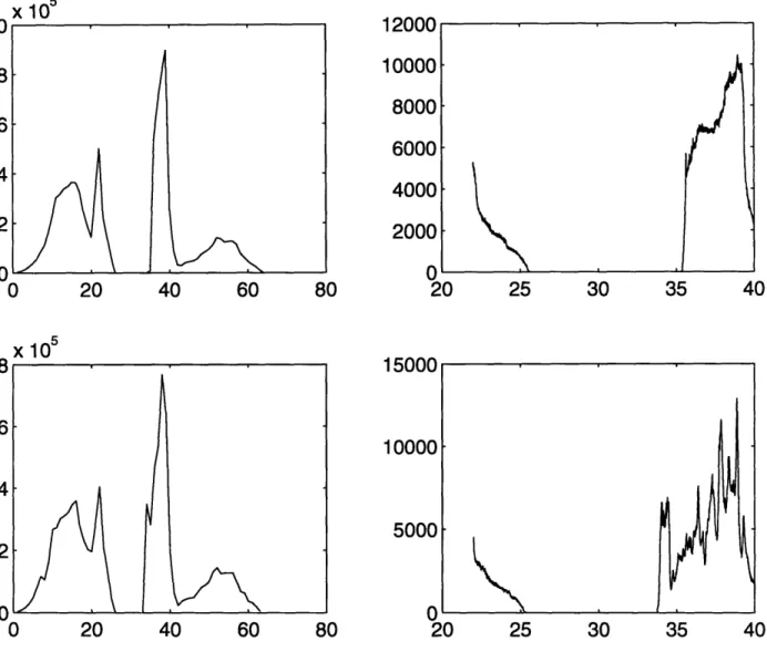
modes ofpal-ladium hydride/deutride. We created a Pd vacancy at ao(1, 1, 1) and observed the
density of states. The results are shown in Figures 3-5 and 3-6.
The results are very interesting. The Pd vacancy has sufficiently s ftened up the
potential for the impurity atoms that a large number of modes have shifted to the
bottom of the optical band. We were hoping for the phonon mode, to be in the
band gap, however we have to remember that we have not taken lat ice relaxation
into account. Pd is a large atom. When we remove it from the cell, 'it will have a
significant effect on the potential seen by the atoms around it. The hop4 is that when
we take lattice relaxation into account, the phonon modes will end u) in the band
gap.
_ _~~~
sites. All of the calculations we did gave us exactly the same answers. Hence this
served as an additional check on our code.
x 10
60
10
20
Figure 3-4: The figure shows the density
Deutride
30
40
50
60
of states for the Fukai structure for Palladium
14
12
10
8
6
4
2
n20
40
60
80
x105
20
40
60
80
12UUU10000
8000
6000
4000
2000
025
30
35
40
I DUUU10000
5000
025
30
35
40
Figure 3-5: The top figures show the density of states for a perfect Palladium Deutride
lattice. The bottom figure shows the density of states with Pd at ao(1, 1, 1) missing
1