Design of a small-scale and off-grid water desalination system using solar thermal heating and mechanical vapor compression

Design of a Small-Scale and Off-Grid Water

Desalination System Using Solar Thermal Heating

and Mechanical Vapor Compression

by

Abdulmohsen Sulaiman Alowayed

Submitted to the Department of Mechanical Engineering

in partial fulfillment of the requirements for the degree of

Master of Science in Mechanical Engineering

at the

MASSACHUSETTS INSTITUTE OF TECHNOLOGY

September 2019

©Massachusetts

Institute of Technology 2019. All rights reserved.

Signature redacted

A u th o r ...

Department of Mechanical Engineering

Aug 15, 2019

Signature redacted

Certified by..

Gang Chen

Carl Richard Soderberg Professor of Power Engineering

Signature redacted

Thesis Supervisor

Accepted by .

Nicolas

Hadjiconstanuiou

Chairman, Department Committe on Gradute Students

OFTECHNOLOGY

SEP

19

2019

LIBRARIES

Design of a Small-Scale and Off-Grid Water Desalination

System Using Solar Thermal Heating and Mechanical Vapor

Compression

by

Abdulmohsen Sulaiman Alowayed

Submitted to the Department of Mechanical Engineering on Aug 15, 2019, in partial fulfillment of the

requirements for the degree of

Master of Science in Mechanical Engineering

Abstract

Water scarcity affects a large group of people across the globe. It diminishes their quality of life and economic activity. Most existing solutions for cheap water desali-nation are not suitable for small-scale applications, and they also generally require infrastructure such as power and plumbing. In this work, a small-scale and off-grid water purification system is proposed. The system utilizes solar energy through both solar thermal collection to rapidly heat up water and solar photovoltaics (PV) to power a mechanical vapor compression system, and is designed for low-cost and high output purification in a minimal footprint. The proposed system was analyzed in both transient warmup and steady state phases separately, and the results were com-bined to develop an expected performance based on the system parameters. A model was developed based on first principles of thermodynamics and water property cor-relations. The device was then optimized using a cost-centered approach. The best ratio of solar collection was found to be 71% solar thermal collector and 29% solar PV. It is expected to produce an output of 15.09 kg/m2_{/day of pure water at a cost}

of 5.3 $/m3, which is competitive with existing technologies at the small scale. A

prototype was constructed as a proof of concept and was tested under simulated solar flux to validate the model.

Thesis Supervisor: Gang Chen

Acknowledgments

I would like to thank Professor Gang Chen for his wisdom and guidance, my colleague Yoichiro Tsurimaki for his help with many aspects of this project, and my family for their continued support throughout my journey. And a special thank you to my loving partner Anna Heidt for making every day better.

Contents

1 Introduction

1.1 Water Scarcity

1.2 Water Purity . . . .

1.3 Fundamentals of Water Purification

1.3.1 Purification Methods...

1.3.2 Minimum Work of Separation

1.3.3 Boiling Point Elevation . . . . . 1.3.4 Recycle of Latent Heat . . . . . 1.4 Current Desalination Technology . . .

1.4.1 Multi-Effect Boiling . . . . 1.4.2 Multi-Stage Flash . . . . 1.4.3 Reverse Osmosis . . . . 1.4.4 Mechanical Vapor Compression 1.4.5 Solar Still . . . .

1.4.6 Cost Comparison . . . .

1.5 Recent Advancements in Solar Water Evaporation .

1.6 Motivation for Solar MVC Approach . . . .

2 Design of a Combined Solar

2.1 Design Goals . . . . 2.2 System Overview . . . . .

2.3 Modeling . . . .

2.3.1 Steady State MVC

Thermal and MVC System

. . . . . . . . . . . . . . . . 15 . . . 15 16 17 17 18 19 20 23 23 24 25 26 27 28 29 30 33 33 34 35 35

2.4 Steady State MVC with Solar Thermal Heating and Heat Loss . . . . 47

2.5 Recovery Ratio . . . . 49

2.6 Daily Output and Warmup Time . . . . 52

2.7 Cost Analysis . . . . 55

2.8 Condensation Heat Exchanger . . . . 57

2.9 Preheating Heat Exchanger . . . . 61

3 Prototype 65 3.1 _{Overview. . . . .} 65

3.2 Solar Absorber Insulation . . . . 66

3.3 Selective Absorber . . . . 67

3.4 Evaporation Basin . . . . 68

3.5 Insulation . . . . 69

3.6 Compressor . . . . 70

3.7 Condensation Heat Exchanger . . . . 71

3.8 Preheater . . . .. . . . . 72 3.9 Simulation . . . . 73 4 Experimental Results 77 4.1 Warmup . . . . 77 4.2 MVC Operation . . . . 78 4.3 System Performance . . . . 80

5 Summary and Future Work 83

List of Figures

1-1 Map of global water scarcity [1] . . . . 16

1-2 Schematic diagram of a work driven purification system . . . . 19

1-3 Boiling point elevation of water at different salinities evaluated at 100 °C . . . . 20

1-4 Schematic diagram of naive direct recycle of latent heat . . . . 21

1-5 Schematic diagram of general multi-stage desalination system . . . . 22

1-6 Schematic diagram of a general vapor compression system . . . . 22

1-7 Schematic diagram of typical multi-effect boiling system [2] . . . . 24

1-8 Schematic diagram of typical multi-stage flash system [2] . . . . 25

1-9 Schematic diagram of typical reverse osmosis system [3] . . . . 25

1-10 Schematic diagram of a typical MVC system [4] . . . . 26

1-11 Schematic diagram of a multi-stage solar still [5] . . . . 28

1-12 Comparison of cost of water for different technologies at different pro-duction scales [6, 7, 8, 9, 10, 11, 12, 13, 14, 15, 16, 17, 18] . . . . 29

1-13 Map of global solar radiation [19] . . . . 30

1-14 Breakdown of costs for common water purification methods [20] . . . 32

2-1 Schematic diagram of proposed solar powered MVC system . . . . 35

2-2 Simple MVC system diagram . . . . 36

2-3 Plot of the calculated temperature of compressed vapor at different compression ratios and compressor efficiencies alongside the saturation temperature at the compressed pressures . . . . 39

2-4 Illustration of the temperature profile along the condensation heat ex-changer . . . .. . 40

2-5 Plot of calculated specific energies in the simple MVC system . . . . 43

2-6 Diagram of simple MVC system with excess vapor release . . . . 44

2-7 Plot of calculated mass flow rate of distillate as a function of

compres-sion ratio for the simple MVC system with vapor release valve. T = 0.7,

x = 0.035 kg/kg . . . .. . . . . 46

2-8 Plot of calculated mass flow rate of distillate as a function of

compres-sion ratio for the simple MVC system with vapor release valve and heat loss. i = 0.7, x = 0.035 kg/kg, UAo,, = 0.3 W/K . . . . 48

2-9 Plot of calculated mass flow rate of distillate as a function of

compres-sion ratio for the simple MVC system with vapor release valve, input

solar thermal heating

QsT

x = 0.035 kg/kg, UAO,, = 0.3 W/K . . . . 49 2-10 Plot of the maximum achievable final salinity in the basin as a function

of compression ratio with the condition that the compressed vapor saturation temperature is greater than brine saturation temperature

by ATHX,min= 2 . . . .. 51

2-11 Plot of the maximum achievable recovery factor as a function of com-pression ratio with the condition that the compressed vapor satu-ration temperature is greater than brine satusatu-ration temperature by

ATHX,min

2-12 Plot of the daily pure water production at a compression ratio of 1.2 with solar PV heating (Qeating = Wpv= 140 W) . . . .54

2-13 Plot of optimized daily pure water production and optimized basin

w ater m ass . . . . 55

2-14 Component cost breakdown of a 1 m2 solar-thermal absorber . . . . . 56 2-15 Plot of cost of water as a function of area ratio of solar thermal collector

to PV solar panel for the proposed system with fixed PV area of 1 m 2 ₅₇

2-16 Cross sectional view of condensation heat exchanger tube . . . . 58 10

2-17 Plot of calculated heat flux across the condensation heat exchanger as

a function of the temperature difference . . . . 61

2-18 Cross sectional view of tube-in-tube preheater . . . . 62

3-1 Image of prototype during operation . . . . 66

3-2 FEP sheets used for insulation of the solar absorber . . . . 67

3-3 Prototype with top layer of insulation and FEP sheets removed . . . 68

3-4 Image of the compressor used in the prototype: a 12 V diaphragm pump 71 3-5 Overhead image of the prototype without insulation . . . . 72

3-6 Close up image of the prototype without insulation . . . . 73

3-7 Heat flow diagram of system warmup . . . . 74

4-1 Solar-thermal heating of the prototype under 2.25kW/m2 _{. . . . 78}

List of Tables

2.1 Design goals for the proposed solar powered MVC system . . . .

3.1 Transient warmup simulation parameters . . . . 34

Chapter 1

Introduction

1.1

Water Scarcity

Water is an important resource for human life. While it may be abundantly available on our planet, it often contains salts and other contaminants and is unsuitable for use. Only about 3% of the worlds water is freshwater and only 0.5% of that is usable as the rest is frozen in glaciers and ice caps [21]. Thus, the majority of water must be purified through one of a multitude of purification methods. However, the purification of water is costly both in energy demand and capital cost, so the supply of pure water struggles to keep up with the rising demand in many regions of the world. This is due in part by rising human populations as well diminishing freshwater supplies due to global warming [21].

According to the World Health Organization, only 71% of the global population has access to a safety managed source of drinking water, the other 29% (2.1 billion people) use sources that are either contaminated, available intermittently, or not located on the premises requiring a round trip commute to obtain

[22].

people, 844 million lack access to basic drinking water services. Figure 1-1 shows the regions of water scarcity. Scarcity is measured by the availability of fresh water per capita. From the figure, we see that areas of water stress are found in parts of South Asia and East Africa, and water scarcity is found in North Africa and the Middle East.

v-y*6r~- ~

~j~inJ1

Soc: FAO. NIOW*st

MM dbimsIn~te( WRI).

PHiUPPE EKACEWCZ

Freshwater availablity,

cubic mtree pperson and per year, 2007. Scarcity

7 Vulnerability

0 1000 1 700 2 500 6 000 15 000 70 000 684 000

JData non available

'I,

Figure 1-1: Map of global water scarcity [1]

Water is used in many sectors including agriculture (irrigation, livestock, fisheries, and aquaculture), industrial use (mines, oil refineries, manufacturing plants, and

power plants), and domestic use (drinking, bathing, cooking, and sanitation) [211. Thus, the availability of clean water affects many aspects of a communitys wellbeing.

Scarcity of water supply has historically led to drought, famine, loss of livelihood,

spread of water-borne diseases, forced migrations, and open conflict [23]. The World

Economic Forum listed water scarcity among the highest global systematic risks [24].

1.2

Water Purity

Water is obtained from many different sources depending on the particular region and the purpose of use. Sources include surface water such as seawater, or water from

lakes, rivers, and ponds and groundwater extracted from wells and aquifers. Water extracted directly from a natural source often contains contaminants that make it

metals, organic chemicals, and microbes [25]. Purification is required to reduce the concentration of contaminants down to a level appropriate for use such that it will not cause adverse effects to those consuming it. A metric for the purity of water is the total dissolved solids (TDS) often measured in weight ratio, parts per thousand (ppt), or parts per million (ppm). The most commonly treated water is seawater whose major dissolved ions are chloride and sodium, followed by sulfate, magnesium, calcium and potassium. The typical seawater TDS concentration is 35 g/kg, although it can reach 50 g/kg in confined coasts

[25].

1.3

Fundamentals of Water Purification

1.3.1

Purification Methods

Purification of water is a work-driven process to separate the liquid water from dis-solved or suspended contaminants. The methods for separation are either based on mechanical separation, thermal separation by phase change, or chemical separation through additives.

Mechanical separation is often done by passing the feed water through a filter. Filters can be as basic as compressed sand or charcoal to nanostructured membranes. Different types of membrane separation methods are characterized by the pore size

[26]. The pore size dictates the minimum size of contaminants that can be removed.

The filters resist water flow through narrow channel friction or osmotic pressure, so a pressure difference must be applied across the filter. Energy is expended as water passes from high to low pressure. Therefore, work is required to maintain the pressure difference in the form of pumping. The most common form of purification

by this method is known as Reverse Osmosis (RO)[26]. Another form of mechanical

separation is electrodialysis (ED), which similarly uses membranes for purification but induces the flow of dissolved ions through the application of an electric potential. Thermal separation is achieved by inducing a phase change in water. When water is evaporated through heating, the vapor can no longer act as a solvent for the

con-taminants and thus the solutes precipitate out. The water vapor is then condensed into pure liquid water while releasing the latent heat. This thermal process requires work in the form of heating to overcome the latent heat of vaporization of water, though some energy can be recovered from condensation heat.

Chemical purification methods vary but include ion exchange, liquid-liquid ex-traction, and gas hydrate precipitation [27]. The methods are not as widely used as the previous methods, particularly for desalination, and are often impractical for treating high levels of TDS.

1.3.2

Minimum Work of Separation

Since mixing is an energetically favorable and irreversible process. Work must be expended to undo the process. The minimal work required for separation is discussed

by Lienhard et. al. [28]. Considering the arbitrary purification system in Figure 1-2,

the two thermodynamic equations are:

+O= (rhh),pre + (rh)brine - (7-4h)feed (1.1)

(7fls)pure + (ThS)brine (TIs)feed + T + Sgen (1.2)

where W is the work input, Q is the heat input, r is the mass flow rate, h is the specific enthalpy, s is the specific entropy, To is the temperature at the interface between the system and the environment, and $gen is the entropy generation. The least work is found by combining the equations to eliminate

Q,

Wmin = (frtg)pure + ((ng)brine - (fThg) feed (1-3)

However, in the case of adiabatic separation, the heat transfer from Equation 1.1

can be eliminated yielding a minimum adiabatic work in Equation 1.4. This minimum work is easily evaluated through enthalpy correlations of saltwater, and eliminates the

Pure Water

Feed Water Purifier

Brine

Figure 1-2: Schematic diagram of a work driven purification system

temperature dependence.

Wnmin,adiabatic (Th)pure +(rhh)brine - (rhI)feed (1.4)

The work of separation increases with salinity as well as with increased recovery ratior= "?pure There is a marginal decrease in the specific work if the pure output

mfeed*

contains some dissolved solids and is not entirely pure. Furthermore, thermal pro-cesses have a higher specific energy demand for purification due to the heat transfer over a gradient.

1.3.3

Boiling Point Elevation

When salts are dissolved in water, the partial pressure of water vapor is reduced. Thus, the temperature at which water reaches saturation is higher than in the case of pure water at the same pressure. This phenomenon is known as boiling point elevation (BPE). BPE is measured in K or °C and can be calculated from the following correlation [29]:

BPE = Ax2 + Bx (1.5)

where A = -4.584 x 104 T2 + 2.823 x 10-2T + 17.95, B = 1.536 x 10-4T2 + 5.267 x

10- 2_T

₊

The valid range for this correlation is 0 << T < 200 °C and 0 < x < 0.12 kg/kg.

Equation 1.5 is plotted in Figure 1-3. For small ranges of salinity the relationship is roughly linear.

2 0 1.75 1.5 -0 1.25 1 I 0.75 P 0.5 -0.25 -0 0 0.02 0.04 0.06 0.08 0.1 0.12 Salinity x (4)

Figure 1-3: Boiling point elevation of water at different salinities evaluated at 100 °C

BPE is relevant for desalination particularly at high recovery rates, because the high salinity brine must be brought to an elevated temperature in order to evaporate.

A desalination system must be design to handle the highest expected BPE.

1.3.4 Recycle of Latent Heat

In a thermal desalination process, it is necessary to evaporate water. The latent heat of vaporization of water is large Ahfg = 2256 kJ/kg, so the energy demand would

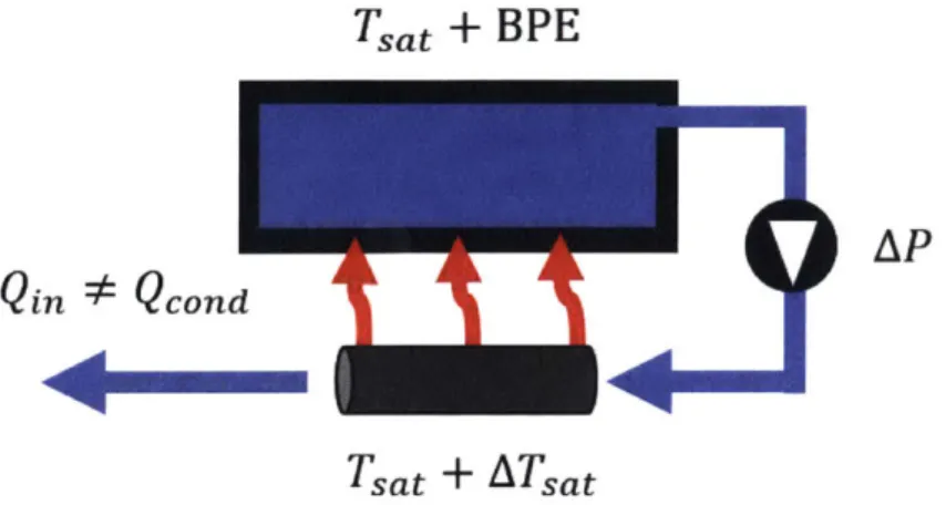
be too high for simple direct evaporation to be a viable method for desalination. However, much of that energy can be recovered when the vapor condenses. The heat from the condensation can be used to evaporate more water and so on. Thus, the energy cost is only the difference between the expended and recovered energy. The recycle of latent heat is a fundamental component of any thermal desalination process. The simple and direct way to attempt to recycle latent heat is depicted in Figure 1-4. Brine water boils in a main chamber and the vapor flows into a condensation tube, where an attempt is made to recycle the condensation heat back into the main

chamber. However, this system does not work, as the boiling point elevation will create a positive temperature gradient such that heat cannot flow back into the brine.

Tsat

+ BPE

12A.

Qin * Qcon

_4*Qond

Lai

y

Tsat + ATsat

Figure 1-4: Schematic diagram of naive direct recycle of latent heat

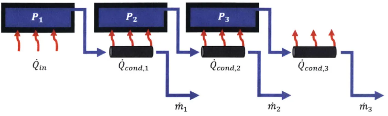
The correct way to achieve latent heat recycle is by controlling the pressure of vapor or water such that the saturation temperature of condensate is greater than that of the evaporate. This is done by either multi-stage systems or by vapor compression. In multi-stage systems, a series of chambers evaporate water at progressively lower pressures such that the vapor from stage n condenses in stage n + 1 and releases its

latent heat. Figure 1-5 shows a simple diagram of a multi-stage system with three stages. It can be extended to an arbitrary number of stages. The water in each stage is at lower pressure than the previous Pi > P2 > P3. The heat transfer from

condensation is slightly lower in each progressive stage due to the energy that goes

into the separation of salt from pure water

Qin

Qcond,

difference is small relative to the value of the heat transfer. The limitation of the multi-stage approach is that the condensation heat from the final stage cannot be reused so it is released into the environment.

The other method for latent heat recycle is through vapor compression. Com-pressing vapor by a pressure AP corresponds to a rise in the saturation temperature ATsat. Supplying enough compression will allow the vapor to condense at a suffi-ciently higher temperature than the evaporate. Figure 1-6 shows a simple diagram of such a system. Vapor compression systems benefit from the simplicity of having only

Qin cond, cond,2 cond,3

1 2 ?h3

Figure 1-5: Schematic diagram of general multi-stage desalination system

a single stage. However, the limitation is the energy expended in compression which, in practice, occurs at a non-ideal efficiency.

Tsat

+

Qin= Qcond

Tsat + ATsat

Figure 1-6: Schematic diagram of a general vapor conipression system

The systems discussed all achieve the goal of improving the energy efficiency of desalination. The efficiency can me measured by the so-called Gain Output Ratio (GOR). GOR is a dimensionless number that represents the ratio of the mass of pro-duced water by the desalination system to the mass of vapor that could be generated

by direct heating. And it is one of the key metrics for thermal desalination systems.

It is calculated using the following equation:

GOR= . (1.6)

Qin

where h is the mass flow rate of distillate, Ahfq is the latent heat of vaporization, and

Q

such as in an electric boiler or single stage solar still. Such as system does not recycle heat from condensation. A higher value of GOR means more pure water is produced for the same amount of input energy. Multi-stage systems such as the one in Figure

1-5 achieve higher GOR with greater number of stages. The maximum GOR of a

multi-stage system with n stages can be estimated by evaluating the sum of mass flow rates as rhi ~ as in Equation 1.7, where the latent heat of vaporization of saline water is approximated as pure water. If we make the approximation that

Qin ~ Qcondi Q

Ocond,2

find that the maximum GOR is equal to the number of stages GORmuitistage,max ~ n. Large-scale desalination plants have GOR of the order of 8

[30.

GORmuitistage _ in +

Ocondense,

Q in

The GOR of the vapor compression system is not bounded by the number of stages and is only limited by the inefficiency of compression, which leads to superheating of the vapor, and the separation energy. It is therefore possible to achieve a high GOR with only one stage and minimal complexity. It is therefore ideally suited for small-scale applications.

1.4

Current Desalination Technology

In this section, we review the most prevalent technologies for desalination as well as some technologies relevant to this project. The methods used are based on the fun-damental methods of purification, but their implementation varies slightly depending on the system scale, feed water condition, desired performance, among other factors.

1.4.1

Multi-Effect Boiling

Multi-Effect Boiling (MEB) is a thermal evaporation-based purification process. It ac-counts for 8.20% of the global desalination capacity [2]. Figure 1-7 shows a schematic

diagram typical MEB system with 3 stages or effects. Input power is supplied by a gas or electric boiler which generates a flow of steam which is used to evaporate the feed water in the first stage. Subsequent stages at lower pressure recycle the latent heat of condensation from the previous stage. Feed water is sprayed onto the condensation pipes to increase surface area and promote better heat exchange. MEB systems often suffer from scale formation from the precipitating salts from the feed water which hinder the heat transfer performance [26].

Note: P, > P2 > P, P= Pressure

Ti > T₂ > T3 T= Temperature

First effect Second effect Third effect

______________________________________ I

Vacuum r-Vacuum E'OVacuumn

Steam

boiler lee apor 0e 0 0 Vapor e e.

Condensate

turned4- •Condensed Condensed

to boiler fresh water fresh water

- - ------------ -Vapor -Oo Note-alFinal condenser T1 > T2 T3 f Saline Vapor U

Figure 1-7: Schematic diagram of typical multi-effect )oililg system

[21

1.4.2

Multi-Stage Flash

Multi-Stage Flash (MSF) distillation accounts for 25.99% of the worlds desalination capacity [2]. It is a thermal evaporation-based process, like MEB, with latent heat recycled through multiple low-pressure stages. It similarly uses a boiler to generate the input flow of steam. Unlike MEB, the saline feed water is evaporated by flashing, a process in which saturated water is partially evaporated by discharge into a lower pressure chamber. The flashing process avoids the used of a heat transfer surface for boiling, and thus avoids the problem of scale formation. Figure 1-8 shows a schematic diagram of a typical MSF system with three stages.

Flash and heat recovery section

First stage Second stage Nth stage

Steam Ejector ejector gP b, ~~ steam '-00M7 istinlate Chemicals added Saline ... . ... ...* feedwater Cooling 11 water Ejector discharge condenso Contaminated condensate Fresh to waste -- o water mdBrine discharge

Figure 1-8: Schematic diagram of typical multi-stage flash system [2]

1.4.3 Reverse Osmosis

Reverse Osmosis (RO), is a membrane-based desalination method and the most preva-lent desalination technology accounting for 59.85% of the global desalination capacity [2]. Figure 1-9 shows a typical configuration of a RO system with two stages. The stages contain the purification membranes, and multiple are used to lower fouling on the initial stages and increase the recovery ratio. High pressure pumps are required to overcome the osmotic pressure of the membranes. Pressure from outflowing brine is recovered through a pressure exchanger to increase the efficiency of the system and lower the required pumping power.

PRO stage I

_QC,

high pressure pump a

stage 2 perme fee-7dmembrane module

booster pump

Qb

pressure exchanger

bri

Figure 1-9: Schematic diagram of typical reverse osmosis system [3]

ate Cb ne Heating section Steam boie rin Condensate returned 4 to boiler

1.4.4

Mechanical Vapor Compression

Mechanical Vapor Compression (MVC) distillation is a thermal evaporation-based process that relies on the heat exchange from pressurized condensate to evaporate in a single chamber. It is less prevalent than the previously discussed technologies because of its relatively high energy requirement. Figure 1-10 shows a schematic diagram of a typical MVC system. Compression of vapor introduces sensible heat which is used to overcome the work of separation and maintain steady state. Therefore, additional heating is not required once the system is started. Feed water is sprayed over condensation tubes similar to the MEB process to increase the surface area and increase the rate of heat transfer. Preheaters are used recycle the sensible heat from the pure condensate and brine water, and heat incoming feed close to the boiling point. demister Evaporator Non-Condensable . Feed Seawater Md, Td Distillate Feed Preheater Product M d, T, Rejected Brine M b, T b Intake Seawater Brine Feed Preheater Brine Mb, _T,

Figure 1-10: Schematic diagram of a typical MVC system [4]

1.4.5 Solar Still

The solar still is perhaps the most basic thermal desalination technology. It operates

by evaporating water through solar heating, and allowing the water to condense

against the slanted glass or plastic top surface of the device. As discussed in the previous sections, direct boiling without heat recycle from the condensate is very energy intensive and thus the single basin solar still has poor efficiency. However, the solar still can be made into a multi-stage system. One method is to stack the evaporation basins on top of each other while using a transparent surface to separate the basins [31]. Another approach depicted in Figure 1-11 separates the solar thermal collector from the evaporation basins. Vacuum pumping is used to create a pressure difference between the stages. However, even with a carefully designed system, the relatively low power density of solar radiation which is on average 1 sun = 1 kW/m2 means that multi-stage solar stills only generation of the order 14 kg/m2/day

[5].

The advantage of a solar still is that the system capital cost is low, but with the low production rate the cost of water becomes impractically high compared to other technologies.

Photo Water stor -volt agetank Stage3 Fresh water Stage2 Stage I

Fresh water tank Brine collection Heaankagc

aic solar collector

Batteries & controllers

Vacuum pump

Pressure control valves

Solar collector

Figure 1-11: Schematic diagram of a multi-stage solar still

[5]

1.4.6 Cost Comparison

The cost of water is perhaps the most important metric for a desalination system. Often measured as dollar per cubic meter, the cost varies by technology and also by the scale of the system. Figure 1-12 shows the cost of water at different scales. The data was taken from numerous sources of published literature. Large-scale desalination plants are cheaper than even the most competitive small-scale systems by about an order of magnitude. This is achieved through the use of highly energy efficient multi-stage systems, and economies of scale. For the small-scale market such as a single household or small community, the options for desalination are of the order of 5

$/m3. Thus, there is an opportunity to develop a system with a low cost of water the

unserved small-scale market.

46-"

0

i..

100

% Solar still (per m2

footprint)

Membrane distillation Humidification

10 -dehumidification Reverse Osmosis + diesel or solar PV

- Large-scale desalination ... . Oppportunity 0.0*

3

Daily production [m3/day]

Figure 1-12: Comparison of cost of water for different technologies at different

pro-duction scales [6, 7, 8, 9, 10, 11, 12, 13, 14, 15, 16, 17, 18

1.5

Recent Advancements in Solar Water

Evapo-ration

Significant research has been conducted into the solar-thermal conversion process due

to its high efficiency. Solar water evaporation is a particular subset of solar-thermal

applications. Several recent developments have been made to improve the conversion efficiency. Interfacial evaporation using a floating structure has been used to

concen-trate the solar heating into a thin layer of water, and avoid heating the bulk water

[32]. Contactless solar water heating was conducted by using a solar absorber which

emits infrared radiation to the water surface [33]. The process results in interfacial heating without the complication of fouling any floating structure. Recently, the use of hydrogels has been reported to lower the latent heat of vaporization of water and lead to a significant increase in evaporation rate [34]. These developments show po-tential highly efficient solar-thermal heating in the future, and incorporation of these

advancements into desalination systems could be valuable.

1.6

Motivation for Solar MVC Approach

In an attempt to improve upon the current desalination technologies, several factors where considered. The foremost of which is the needs of the user, in this case, those living in rural or off-grid locations as well as in regions of water scarcity. Such loca-tions suffer from unavailable or unreliable sources of power, and thus the desalination system must be powered by an abundant and renewable energy source. One of the most promising power sources is solar radiation. Figure 1-13 shows the incident power density of solar radiation across the globe. We can see that many of the same regions affected by water scarcity from Figure 1-1 also observe relatively high solar incidence, around 6 kWh/m2_{/day or above. For this reason, solar was selected as power source}

for the desalination system, and as such the approach will take advantage benefits of available solar harvesting devices.

SOLAR RESOURCE MAP X WORLDBANKGROUP E

GLOBAL HORIZONTAL IRRADIATION %.

=-=

Yay sm: < 803 949 5 124 1387E 18 451 NE 90 1051 1201 > 45'N O0N 5% 15s Vtj

Long-termaverage of daily/yearly sum

Dalysum: ra2.2 2.6 3.0 3.4 3.8 4.2 4.6 5.0 5.4 5.8 6.2 6.6 7.0 7.4

~~k~h/m'

Yearlysum: <803 949 1095 1241 1387 1534 1680 1826 1972 2118 2264 2410 2556 2702 >

Thismrap is published by the World Bank Group, funded by ESMAP. and prepared by Sotaris. For more informsanand terms of use. plesevisit http://baorats~nfo.

Figure 1-13: Map of global solar radiation [19]

system to be easily maintained on site with available tools and materials. Membrane based desalination methods such as RO require frequent replacement of membranes after a set volume of water has been purified. Membrane replacement accounts for

50% of costs in large-scale seawater RO plants

[35].

Large-scale desalination systems such as MSF and MEB are unsuitable for small-scale implementation. The efficiency of such systems relies on having multiple stages at progressively lower pressures. Typical large-scale plants have 20 to 30 stages [36]. The complexity associated with the high number of stages will increase the capital cost of the desalination system. For large production rates, the impact the complexity has on cost is reduced due to economies of scale, but for low production rates the impact on cost is more prominent. The stages are also designed to withstand vacuum pressures below 0.1 bar [37], which incurs significant capital cost and manufacture complexity.

Among the common desalination technologies, MVC has a high cost due to its electrical energy consumption (see Figure 1-14). Whereas other technologies, such as RO, have relatively higher costs of operation and maintenance. There is not much that can be done from a system design standpoint to improve the maintenance costs of RO, which are largely based on membrane replacement [20]. However, the energy consumption costs of MVC, which is around 11 kWh/m3, can be reduced

closer to the theoretical limit and thus produce a significant cost saving. This is attempted in this work, by careful modeling of the energy flow through the MVC system, and incorporation of solar power through solar photovoltaics (PV) and solar-thermal collectors to satisfy the energy consumption needs.

A final consideration for the selection of MVC as the base technology for the

proposed solar powered desalination system, is that MVC achieves full recycle of the latent heat of condensation with only a single stage. The reduced complexity in number of stages can give a lower capital cost, and similarly reduced system size.

1.0

G Electrical Energy (see Notes A & B) 0.9 oThermal Energy (see Note C)

* Operation and maintenance costs excluding energy (see Notes D. E & F)

0.8 a Capital cost of desalination plant (see Note G)

E Cost of finance (see Note H)

0.7 0.6 E 0.5 ---0.4 0 .3 -- -- - -- -0.2 0.1

Electrodlalysis (Brackish) Reverse Osmosis Reverse Osmosis Multi-Effect Boling Multi-Stage Flash Mechanical Vapour (Brackish) (Seawater) (Seawater) (Seawater) Compression

Figure 1-14: Breakdown of costs for common water purification methods

[20

_[43.

Therefore, relatively simple heat exchangers and common pipe fittings can be used which simplify the design and maintenance.

Chapter 2

Design of a

Combined

Solar

Thermal and MVC System

2.1

Design Goals

Any good design must be developed according to particular design goals and have a metric for measuring the performance with respect to each goal. The goals for the system are listed in Table 2.1. The cost metric was chosen to be competitive with existing cost of water at the proposed small-scale production quantities. The system is also made to be self-sufficient, and not have to interface with a power source or urban infrastructure. In addition, the system should not require specific replacement parts (such as membranes for RO systems) that may be difficult or costly to obtain in rural regions. And finally, we do not forget that solar radiation is a relatively dilute power source, so the system must have good performance in minimal footprint owing to the opportunity cost of land, whether it is open ground or a rooftop.

Table 2.1: Design goals for the proposed solar powered MVC system Design Goal Metric Units Target

Low cost _{Total Expected Water Production} Capital Cost _m$ 3 <5-L m3

Reliance on grid power

Off grid - None

Reliance on existing infrastructure

Easy to maintain Number of exotic replacement parts - None

Small footprint Daily water production kg > 15

System footprint m2day

2.2

System Overview

The proposed system is depicted graphically in Figure 2-1. It consists of a single evaporation basin. The top of the basin features a selective solar absorber to heat the water and begin evaporation. Above the solar absorber is a set of transparent plas-tic sheets that insulate the absorber and reduce convective heat loss. A compressor is connected to the basin and it compresses the vapor and allows it to condense at a higher temperature in the condensation heat exchanger which passes through the basin. Excess vapor can be released by a vapor release port or valve such that the basin remains at ambient pressure. Feed water is supplied by an attached reservoir whose water level is kept constant by a controlled inflow of feed water. The feed is preheated prior to entering the evaporation basin by a counter flow heat exchanger. The condensate passes through the feed reservoir itself to ensure all vapor is con-densed if the previous heat exchangers were not effective enough. The outlet of the system contains a pressure control valve, such as a relief valve, to achieve the desired compressed vapor pressure. Finally, the evaporation basin, and both heat exchangers are surrounded by insulation to limit heat loss.

Typical MVC systems feature a brine outlet port where non evaporated feed is released at a constant flow rate. This is done to conserve the recovery ratio and maintain salinity in the chamber. The proposed system does not require a constant

brine outflow because it is designed to be operated intermittently during available sunlight. Thus, the brine need only be flushed out at night, the mechanism for which is not included in the analysis but is necessary to have in the final system.

Transparent plastic sheets

Selective absorber

PV solar Compressor

panel Vapor release Ogeo-* -1 1 --AO'Ovalve

00 14- Vapor flow

Pressure Condensation

control valve heat exchanger

Pure water

Feed reservoir _Preheater

Figure 2-1: Schematic diagram of proposed solar powered MVC system

2.3

Modeling

2.3.1

Steady State MVC

The basis of the proposed device is a MVC system powered by a PV solar panel. Therefore, we first devise a model for the MVC system using energy balance. MVC has been extensively modeled using fundamental mass and energy equations, water property correlations, as well as the method of exergy [4, 38]. However, this system is a simplified version of MVC which does not feature brine outflow, and thus a new model is developed based on a similar approach. To fix the scale of the system, we will assume it is powered by a 1 m2 PV solar panel with an efficiency of 14%. Figure 2-2 shows a simple diagram of the MVC aspect of the system where the dotted box outlines the control volume to be considered. The preheater is excluded from the control volume, but its effect on the system will be accounted for in terms of the input temperature T2 which depends on the effectiveness of the preheater Epreheater.

their efficiencies and other characteristics will be accounted for by substitution into the fundamental energy balance. It must be noted that as the system operates, the salinity of the water in the basin increases as water evaporates. This will cause a rise in the temperature T3 until evaporation stops. In this section we are concerned with

simple steady state before reaching this point. The energy balance for the system in steady state is as follows:

rnhxfeedT₂ - Thhvapor,T₄+ hvapor,T₅- 'Thpure,T_{6 =} 0 (2.1)

where n is the mass flow rate through the system, h is the enthalpy of water at a particular salinity x and temperature T. Pure water corresponds to a salinity of x = 0

kg/kg.

Compressor

Steam flow

|

Pure

water

,WMT1

Preheater

Feed

water

Figure 2-2: Simple MVC system diagram

The temperature T1 is the temperature of incoming feed water which is assumed

to be at equilibrium with the ambient temperature outside the system. A typical

ambient temperature of 25°C is used.

The temperature T2 is the temperature of the feed

the preheater heat exchanger. Given the effectiveness of fact that the flow rates and specific heat capacities of temperature can be calculated as follows:

q _Ce (T,₀nt - T~n)

Epreheater-

-qmax Cmin (Th,in -Tc,in)

T2 =T₁+ 6_{preheater (T} 6 - T1)

water after passing through the heat exchanger, and the both streams are equal, the

(2.3)

T2 -T 1

T6 -- T1

(2.4)

The temperature T3 is the bulk temperature of the brine water in the basin. The

water in the basin is at saturation at atmospheric pressure during steady state. The temperature is thus dependent only on the salinity in the basin x. The starting salinity is the salinity of the feed seawater Xinitial = Xfeed= 0.035 kg/kg, which corresponds

to a starting temperature of T3 = 100.49 °C. In general, T3 is evaluated by adding

the pure saturation temperature to the boiling point elevation from Equation 1.5.

T3= Tsat,Patm+ BPE = 1000C + BPE (2.5)

The temperature T4 is the temperature of saturated vapor evaluated at

atmo-spheric pressure Patm = 1 atm = 101.325 kPa, which is the pressure inside the basin.

T4= Tsat,pat = 100C (2.6)

The temperature T5 is the temperature of superheated vapor after undergoing

compression. Given a compression ratioP , the ideal temperature after isentropic compression can be calculated by adiabatic compression of an ideal gas as follows:

P

-T5,ideal= T4 (P ) (2.7)

where y is the ratio of specific heats and is equal to 7 = 1.33 for pure steam. The

actual temperature of the outlet vapor from the compressor will be higher due to entropy generation which can be characterized by the efficiency. For the case of a compressor, the efficiency is defined as the isentropic enthalpy change divided by the ideal enthalpy change of the compressed fluid at the same pressure difference, and is approximated as the isentropic temperature change divided by the actual temperature

by assuming a constant specific heat of vapor cy,.

(h5 - h4)ideal c,, (T5 T4)ideal _ T5,ideal - T4 _(2.8)

(h5 - h4)actal CpV (T 5- T4)actual T5 - T4

From Equations 2.7 and 2.8, we can calculate the temperature of compressed vapor at different compression ratios as follows:

T5 = T4 (Pat'

)+1

After compression, the superheated vapor flows through the condensation heat exchanger and condenses to liquid water while releasing the sensible and latent heat. The condensation heat exchanger is designed to have a sufficiently high overall heat transfer coefficient UA such that all vapor can be assumed to reach saturation temper-ature and condense to liquid water. Thus, the tempertemper-ature of the outflowing liquid

water from the condensation heat exchanger T6 depends only on the compression

ratio.

T6 = Tsat,P, (2.10)

The temperature of saturated water can be calculated by solving the pure water correlation for partial vapor pressure and equating it to the compressed pressure in

In (P,) = a

+

where ai = -5800, a2 = 1.391, a3 = -4.846 x 10-2, a4 = 4.176 x 10- 5, a5 =

-1.445 x 10-", a6 = 6.545. The pressure is calculated in Pa and the temperature is

given in K. The valid range is 100 °C < T < 300 °C.

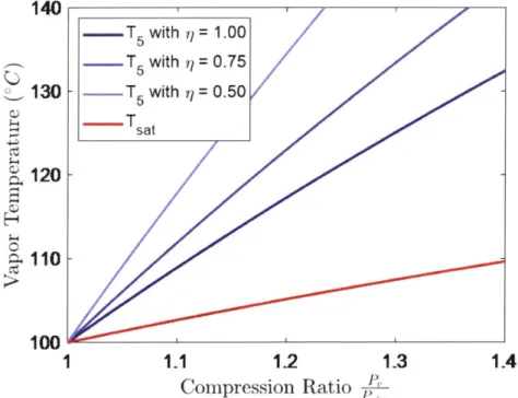
Equations 2.9 and 2.11 are plotted in Figure 2-3. We notice that the temperature

after compression is always greater than saturation, thus the vapor is superheated, and that a reduction in compressor efficiency leads to greater superheating.

140 _____ .-- T 5 with r/ = 1.00 .-.- T5 with 77 = 0.75 _130 - T with = 0.50 -sat 0120-110 100 1 1.1 1.2 1.3 1.4 Compression Ratio P

Figure 2-3: Plot of the calculated temperature of compressed vapor at different com-pression ratios and compressor efficiencies alongside the saturation temperature at the compressed pressures

Additionally, we impose a condition on the temperature T₆ such that the as-sumption of full latent heat recycle is valid. The condition is that the temperature difference across the condensation heat exchanger ATHX is greater than a minimum value ATHX,mi = 2 °C. The heat exchanger will then be designed to accommodate the required heat transfer given the minimum temperature difference.

Temperature T5

T6--T --- ITHX

Distance

Steam Two-Phase Liquid

Figure 2-4: Illustration of the temperature profile along the condensation heat ex-changer

ATHX = T6 -'I3 _> ATIXmiin (2.12)

Figure 2-4 shows the expected temperature progression of the condensate through the heat exchanger. The majority of the heat transfer will be from the two-phase state, however there is sensible heat released from the superheated vapor. The liquid water is assumed to flow out after condensation quick enough as to not release any sensible heat.

After developing an expression for each of the necessary temperatures, we

at-tempt to simplify Equation 2.1 by evaluating the enthalpies. This is done by first realizing that the difference in enthalpy between outflowing distillate and inflowing

feed represents the power expended by the system to purify water Wpurify. Similarly, the difference in enthalpy of vapor before and after the compressor represents the compressor power Wcomp, such that Equation 2.1 becomes:

Wcomp - Wpurify=0 (.

where

Wpurify = n (hpure,T6- hxfeed,T2) (2.14)

Wcomp = i (hvapor,T5- hvapor,T4) (2.15)

The difference in enthalpy between saline and pure water is considered and calcu-lated using the following correlation for seawater [29]:

h,T= hpure,T- Ahsalinity,x,T (2.16)

where

Ahsalinity,x,T= (x (27062.623 + x) + x (4835.675 + x) x T) (2.17)

In this correlation, Ahsalinity,xT is in J, the temperature T is in °C, and the

salinity x is in kg/kg. The valid range for this correlation is 10 °C < T < 120 °C, and 0 < x < 0.12 kg/kg. Ahsalinity,x,T represents the specific energy of mixing and must be overcome to separate pure water from the brine. It depends on the salinity and the temperature at which it is evaluated. However, temperature dependence is relatively small. In the range of 90 °C < T < 110 °C, Ahalinity varies by 0.42%. Thus, we will approximate it by evaluating it at T = 100 °C, as in Equation 2.18.

Ahsalinity,x,T Ahsaunity,x = X(27062.623 + x) + x (4835.675 + x) x (100) (2.18)

The specific energy of purification can be expanded and split into two terms:

= cp,i (T6- T2) + Ahsalinity,xfeed (2.19)

where ck = 4.22 gk is the specific heat of water evaluated at 100 °C. The work

of purification goes towards additional heating of the feed to overcome the limited

effectiveness of the preheater and towards separation of pure water from the brine. It can be simplified by substitution of Equation 2.4 into the expression.

purify c,(1- Epreheater) (T6- T1) + Ahsauniy, (2.20)

The specific work of the compressor from Equation 2.15 can be expressed using the specific heat of vapor c,,, = 1.89 _kgKkJ evaluated at 100 °C, and simplified using

Equation 2.9.

cpv (T5 - T4) = c,,T4 "(2.21)

m _r.

The specific energy of purification and compression from Equations 2.20 and 2.21 are calculated and plotted in Figure 2-5 as a function of the rise in saturation tem-perature, which is directly related to the compression ratio. The compressor specific work is compared to the calculation by M. A. Darwish [39]. According to the energy balance, the two specific works must be equal in order to maintain steady state op-eration. Thus, there is only one value of compression ratio for which steady state is viable and it can be found at the intersection of the lines in Figure 2-5. If the com-pression ratio is too low, then not enough energy is supplied to maintain evaporation and the mass flow rate will drop to zero. If the compression ratio is too high then too much energy is supplied for evaporation and there will be a buildup of vapor in the basin, which will lead to pressurization of the basin fluid and possible rupture of the basin. This limited operating range makes the system highly unstable.

140 _ _ _ _1_1_1 - Purify,e,,haeer 1 120 - Purify, re,ccr = 0.9 - Purify, cpreheater 0.8 1 -Comp, r = 0.7 -- Comp, M.A. Darwish . 8 0

-

60-

20-0

0 2 4 6 8 10 12

Rise in Saturation Temperature Tsat (°C)

Figure 2-5: Plot of calculated specific energies in the simple MVC system

To solve this problem and expand the operating range of the system, a pressure relief valve is added to the basin which will release excess vapor to maintain the atmospheric pressure and release excess energy. The release valve is shown in the diagram in Figure 2-6. The effects this modification has on the system must be

considered. The revised energy balance is as follows:

(ri + f1Irelease) hxfec,T2 - 'tivapor,T4 + 5 T - tvapor,TIflreleaselvapor,T4 =

(2.22)

The equation can be split into the following terms:

Wcomp - Wpurify - Wrelease 0 (2.23)

where

release = Trelease (hvapor,T4- hxfeed,T2) (2.24)

The power of released vapor Wrejeaseacts as a sink for excess energy. The mass flow

rate of release vapor rrelease will reach the necessary value to balance the equation. Thus, we need only adhere to the following inequality of energy in order to maintain steady state: Wcomp - Wpurify > 0 (2.25)

Compressor

---

Steam flow

I

Pure

I

water

II1

Preheater

tit

Feed

water

Figure 2-6: Diagram of simplel MVC system with excess vapor release

The release of vapor has two notable effects on the system. One is the increase of feed flow rate which will affect the operation of the preheater, as the counterflow streams will not have equal mass flow rates. The second is the increase of salinity of the brine in the basin due to additional evaporation. To identify whether these effects are significant, we consider the ratio of the released vapor to the mass flow rate of

Vrelease = cp, 1(Tsat,Pam - T2) + Ahfg + Ahsalinity _(2.26) mrelease

The specific energy is dominated by the latent heat of vaporization Ahfg = 2256

kJ/kg which is several orders of magnitude greater than the other terms which are

of the order of 10 kJ/kg. Thus, it simplifies to:

Wree" Ahf _(2.27)

mrelease

By substitution into the energy balance of Equation 2.23, the ratio of mass flow

rates can be calculated as follows:

Wcomp - Wpurify

release = n _(2.28)

Consider the simple MVC system with epreheater= 0.9 and i = 0.7. The optimal

rise in saturation temperature can be found in Figure 2-5 and is ATat = 5.75 °C

which corresponds to a compression ratio of Pv = 1.22. If the compression ratio Patm

is increased by 10%, there will be an excess of specific energy equal to 24.0 kJ/kg. Estimating the ratio of mass flow rate of released vapor to mass flow rate of distillate

by Equation 2.28, we find release = 1.1%. Therefore, the mass flow of released vapor

is small enough as to be neglected compared to the mass flow rate of distillate. Thus, the impact it has on the system performance is negligible.

The mass flow rate can be calculated by equating the vapor compressing power to the compressor power source (the PV solar panel).

Wcomp = ?7PVjsolarApv (2.29)

where QpV = 14% is the efficiency of the PV solar panel,

dsolar=

compression energy in Equation 2.21, the steady state distillate mass flow rate can then be calculated as follows:

= rvsolarApv _(2.30)

T( PV )

-The mass flow rate is contingent upon several conditions developed through the

analysis. Specifically, the energy inequality in Equation 2.25 and the minimum heat

exchanger temperature difference in Equation 2.12. Under those conditions the mass flow rate is calculated and plotted in Figure 2-7. The preheater effectiveness changes the available range of compression ratio, for which a greater effectiveness can lead to higher flow rate. When operating at a compression ratio higher than necessary, there is an excess of input energy and the limit on mass flow rate is dictated by the compressor power source and not by the effectiveness of the preheater.

Figure 2-7 also shows that the mass flow rate decreases monotonically with com-pression ratio. Thus, it is of interest to find the lowest comcom-pression ratio for steady state operation because that will yield the greatest output of pure water.

12 Epreheater ₁ 4preheater 0.9 10 10- Eprheatr =0.8. -8 4 2-0 1 1.1 1.2 1.3 1.4 1.5 1.6 Compression Ratio P

Figure 2-7: Plot of calculated mass flow rate of distillate as a function of compression ratio for the simple MVC system with vapor release valve. r/= 0.7, x = 0.035 kg/kg