HAL Id: halshs-00564573
https://halshs.archives-ouvertes.fr/halshs-00564573
Preprint submitted on 9 Feb 2011HAL is a multi-disciplinary open access archive for the deposit and dissemination of sci-entific research documents, whether they are pub-lished or not. The documents may come from teaching and research institutions in France or abroad, or from public or private research centers.
L’archive ouverte pluridisciplinaire HAL, est destinée au dépôt et à la diffusion de documents scientifiques de niveau recherche, publiés ou non, émanant des établissements d’enseignement et de recherche français ou étrangers, des laboratoires publics ou privés.
Sylviane Guillaumont Jeanneney, Kangni Kpodar
To cite this version:
Sylviane Guillaumont Jeanneney, Kangni Kpodar. Financial Development, Financial Instability and Poverty. 2011. �halshs-00564573�
Document de travail de la série Etudes et Documents
E 2006.7
Financial Development, Financial Instability and Poverty
Sylviane Guillaumont Jeanneney* and Kangni Kpodar**
4th January 2006 35 p. * CERDI-CNRS - University of Auvergne, CSAE, University of Oxford
** CERDI-CNRS - University of Auvergne
Corresponding author: Sylviane Guillaumont Jeanneney Professeur
CERDI-CNRS, Université d'Auvergne 65 Boulevard François Mitterrand 63000 Clermont Ferrand - FRANCE
Tel: (+33-4) 73177405 - Fax: (+33-4) 73177428. mail at: [email protected]
The authors are grateful to the participants in the sixth conference of the Economic Analysis and Development Network (Marrakech, March 2004), for useful comments. In addition, the authors would like to thank the participants in the congress of the Canadian Economic Sciences Society (La Malbaie, May 2005) for helpful discussions.
Financial Development, Financial Instability and Poverty
Summary: This article investigates how financial development is beneficial to the reduction
of poverty, on the one hand by promoting growth and in the other hand directly by the McKinnon conduit effect. At the same time, however, financial instability which accompanies financial development is detrimental to the poor and dampens the positive effect of financial development on the reduction of poverty. These hypotheses are tested successfully on a sample of developing countries over the period 1966-2000, resulting in straightforward policy implications.
I. Introduction
Many studies in the past and in recent years concern the relationship between financial development and growth1 (Roubini and Sala-i-Martin, 1992; King and Levine, 1993; Easterly,
1993; Pagano, 1993; Gertler and Rose, 1994; Levine, 1997; Levine, Loayza and Beck, 2000; Khan and Senhadji, 2003; Chistopoulos and Tsionas, 2004). But until now the question of whether financial development contributes to reducing poverty has been the subject of little empirical work in economic literature (some exceptions are Dollar and Kraay (2002), Honohan (2004) and Beck, Demirgüç-Kunt and Levine (2004).
Evidently the impact of financial development on economic growth and its impact on the reduction of poverty are related issues, as growth is a powerful way to reduce poverty (Bruno, Ravaillon and Squire, 1998). However, it is possible that in certain countries the benefit of growth for the poor is undermined or even offset by the increases in inequality which may accompany growth. As Kanbur (2001)2 underlined, there are many empirical demonstrations that growth in real national per capita income is correlated across countries and over time with reductions in the measure of income poverty on a national level, but “the real dispute is about consequences of alternative politics”. This is why we focus here on the specific impact of financial development on poverty.
We adopt a macroeconomic approach. As Ravallion (2001)3 has underlined, “there is a need of deep microeconomic work on growth and distributional change” in order to define better the more pro-poor policies. In the field of finance, there are already many microeconomic studies concerning the need for specific institutions for the poor, such as microfinance institutions. But to understand better “the large differences between countries in how much poor people share in growth”, macroeconomic analyses are still useful as they may indicate the most pro-poor growth-oriented policies from a comparative perspective, even if econometric cross-sectional analysis faces several limitations.
As in the existing literature, we try to distinguish the indirect effect of financial development on poverty reduction through its positive action on growth from its direct impact. However, two features of our analysis set it apart from the existing literature. First, we are interested by
1 The pioneer work is that of Gurley and Shaw (1960). 2 p.1090-1091
the channels (credit or money) through which poor people benefit from formal financial intermediation. Therefore we focus on the motive of finance for money demand suggested by Keynes (1937) and rehabilitated by McKinnon in 1973 when he presented the “conduit effect”. According to this assumption, even if financial institutions do not provide credit to poor people confined to self-financed investment, they are useful to them in so far as they offer some profitable financial opportunities for their savings. Consequently we do not only focus on a credit indicator as in Dollar and Kraay (2002), Honohan (2004) and Beck et al. (2004), but we also examine the impact of a liquidity indicator. Second, we consider that financial development is accompanied by crises; these are likely to undermine the potential benefits of financial growth, in particular for the poorest. Therefore, besides the indicator of financial development in the regression explaining poverty, we introduce an indicator of financial instability in order to reconcile the apparent contradiction between two schools of thought in the literature, the first underlining the positive effect of financial development on growth while the second shows that credit growth is one of the predictors of banking and currency crises (Loayza and Ranciere, 2002).4
We mainly adopt Dollar and Kraay’s model specification where aggregate poverty is measured by the average per capita income of the poorest population and depends on the level of real GDP per capita and other variables, which in our case integrates financial development and instability indicators. We estimate our model on as large a sample of developing countries as possible over the period 1966-2000. We use panel data and System GMM estimator in order to control for the heterogeneity of countries and the potential endogeneity of the explanatory variables. In addition, following Honohan (2004), we estimate a second model where poverty is measured by the share of the population earning less than one dollar per day. Despite the small size of the sample, this estimation is done in order to check the robustness of our results. We cannot refute the null hypothesis that financial development is on average good for the poor while the financial instability accompanying financial development is detrimental to them. This result only holds when financial development is measured by the ratio of money to GDP and not by a credit ratio; this may be interpreted as evidence of the relevance of the conduit effect assumption.
4 The relationship between financial development and instability may be explained by several factors (for a survey, see Andersen and Tarp 2003); it is the main reason why some authors cast theoretical as well as empirical doubt on the beneficial effect of financial development on growth (Ram, 1999; Demetriades and Hussein, 1996) However, mainstream thought supports a positive impact (see notably Levine, Loayza and Beck, 2000; Chistopoulos and Tsionas, 2004).
The paper is organised as follows. Section two presents the theoretical arguments according to which financial development may exert a direct positive impact on the income of the poor independent of its action through economic growth, while financial instability would be predominantly detrimental to the poor. The subsequent section presents the results of the econometric estimations, based on the two measures of poverty.
II. How does financial development affect the poor? The predominant McKinnon conduit effect
Financial development may exert a positive impact upon the income of the poor in two respects. First, because it boosts economic growth and growth is good for the poor. As previously noted, there is an abundant literature on the relationship between finance and growth (for a survey of the main theoretical arguments, see Levine, 1997). Jalilian and Kirkpatrick (2002) have underlined this indirect channel by which finance reduces poverty. Second, even if access to financial services for the poor is actually more limited than the access for the rest of the population, it may nevertheless be improved by financial development. Here, we are specifically interested by this direct potential effect of financial development on the reduction of poverty.
Why financial development may directly improve the well-being of the poor?
Borrowing is often a requirement for investment in physical capital or in human resources and for insulating expenditure against external shocks. As many authors claim, credit constraints are chiefly binding on the poor (Banerjee and Newman, 1993; Aghion and Bolton, 1997). However, the access of poor households to bank credit may be impeded by the high unit cost of small loans and so financial development may be regressive for the poor. This is the prediction of the well-known model developed by Greenwood and Jovanovic (1990) at the early stage of development. According to this model, benefiting from the screening and risk pooling that financial intermediation offers requires an initial set-up cost that poor households cannot afford. As they are not in a position to use their savings for this outlay, they fall further below in the income distribution. This is why international aid is largely involved in the implementation of micro-credit institutions, the financial equilibrium of which is problematic. However, according to the same authors, access to credit becomes easier over time for the
poorer segments of the population; this may result in an inverted U-shape curve of income inequality and financial development.
Indeed, in so far as the financial system is becoming healthier, powerful and competitive, it is possible that a greater capacity and desire exists to bear the high costs of small credits (Rajan and Zingales, 2003). For instance, in Latin America, commercial banks have begun to make pooled loans available to the poor, as previously experienced by micro-credit institutions (Mosley, 1999). Moreover, the development of informal credit, which is often the only source of borrowing for poor people, is made easier by the growth of the formal financial system which offers opportunities of profitable investments to informal financial institutions or agents. Finally, in a framework of competitive markets of goods and production factors, credit may improve the well-being of the poor, even if they do not directly receive the loans (Beck
et al., 2004)
From our point of view, a second argument seems to be more relevant to support the hypothesis of a beneficial effect of financial development on the poor. A geographically dispersed financial system in a context of small inflation may at least offer the opportunity of demand or savings deposits with a non negative real remuneration or a small real positive one to poor households and small firms. As McKinnon (1973) has emphasized, when the economic units are confined to self-finance so that there is no useful distinction between savers (households) and investors (firms), the indivisibilities in investment are of considerable importance. In this case, money and capital become complementary. “If the real return on holding money increases, so will self financed investment over a significant range of investment opportunities. The increased desirability of holding cash balances (for the poor) reduces the opportunity cost of saving internally for the eventual purchase of capital goods from outside the firm-household. The financial “conduit” for capital accumulation is thereby enlarged”.5
The empirical literature to date has focused, with some success, on the complementary hypothesis of McKinnon which implies that the demand for real money balances depends positively on real income, the real rate of interest on bank deposits and the real return on capital, and that simultaneously the investment ratio is positively related to the real return on
money balances (Fry, 1978, 1988; de Melo and Tybout, 1986; Edwards, 1988; Ajewole, 1989; Laumas, 1990; Thornton and Poudyal, 1990; Morisset, 1993; Khan and Hasan, 1998; Kar and Pentecost, 2001). Here we only take into account the hypothesis that money and capital are complements in developing countries because, in the absence of deep financial markets and extensive intermediation, money balances have to be accumulated before indivisible investment can be undertaken and we consider that the liquidity constraint applies mainly to poor people’s investment. We will try to discriminate between the two channels by which financial intermediation may help the poor: currencies and deposits on the one hand and credits on the other.
The “conduit effect” of real money balances is the main reason why, at the beginning of the seventies, McKinnon advocated freeing the financial systems of developing countries from the constraints which impede their development, such as ceilings on interest rates, high reserve requirements, administrative credit allocation and other government-induced distortions. However, the flip side of the beneficial impact of financial development for the poorest part of the population is probably the detrimental impact of the disturbances of the financial system on said population.
Why does financial instability hurt the poor relatively more than the rich?
Several reasons support the assumption that the poor are more vulnerable to banking crises than the rich. Indeed poor people are particularly hurt by the disruption of the payment system and unwarranted bank closures. The freezing of deposits is particularly detrimental to them as they are unable to diversify their assets and notably invest their savings in foreign banks. In countries where some banks are periodically unable to ensure the liquidity of their deposits, the “conduit effect” suggested by McKinnon is probably dampened or even cancelled out by the doubt surrounding the health of the banking system. Moreover, when banks are in difficulty, they begin to ration small borrowers as these loans are the less profitable for the banks and because poor people have little power of negotiation.
Apart from this direct effect of financial instability upon poor people, we may also assume an indirect effect resulting from the fact that financial instability induces growth instability. Indeed, as the rate of investment depends on the availability of finance, financial instability induces the instability of this rate and therefore that of the rate of growth. Furthermore,
financial instability leads to a volatility of relative prices since the prices of the different goods or services are not influenced in the same proportion by a credit variation: tradable goods prices are determined by foreign prices and the nominal exchange rate while non-tradable goods prices depend on the domestic supply and demand and so are more directly linked to the credit level. Both these instabilities (that of the rate of investment and that of the real exchange rate) lead to growth volatility.
We recall that a negative relationship between the average rate of growth and the volatility of annual rates has been evidenced across countries (Ramey and Ramey, 1995). So it is likely that financial instability inducing growth volatility impedes economic growth.6 As economic growth is a necessary condition for sustainable poverty reduction, financial instability hurts the poor through its detrimental impact on growth. Moreover, poor people may be more vulnerable to the cyclical nature of economic growth than the rich, due to the asymmetry between periods of falling and rising aggregate income; falling periods reduce the income of the poor more than the rising ones improve it. For instance, de Janvry and Sadoulet (2000), using data about twelve countries in Latin America from 1970 to 1994, have shown that economic growth has reduced rural and urban poverty on average, but that the negative impact of regressions on poverty has been stronger than the positive impact of expansions. The reasons for this potential asymmetry of change in income on poverty still have to be elucidated. It is probably the result of several factors which may differ from one country to another. On the one hand the less skilled and poorest workers, being made redundant first, have been unemployed for the longest time when the new expansion begins. There exists histereses effect whereby the former unemployed people are the last to be hired. On the other hand, while prices rarely fall during recessions, they most often rise during expansions, all the more so as the expansions are rapid. As the poor may depend more than the rich on state determined income that is not fully indexed to inflation, such as pension, state subsidies or direct transfers (Easterly and Fischer, 2001), growth fluctuations tend to increase income inequality. Although poverty is generally concentrated in rural areas, governments often do not transmit the rise in international prices of agricultural exports to peasants whereas they do transmit the fall in prices to them, as a result of budgetary constraints. From a more general
6The volatility of the rate of investment and the volatility of relative price (notably real exchange rate volatility) which accompany financial disturbances have been shown to be factors of poor growth performance
point of view, as they do not benefit from an insurance scheme, the fall in poor people’s income may cause them to pay less attention to their health or their children’s schooling, which durably damages their human capital.
On the other hand, in several African countries, it appears that “where there has been recession, mean and redistribution income effects typically have opposite signs, and the redistribution effect substantially mitigates the poverty increasing impact of lower mean incomes (in Madagascar, Nigeria, and Zimbabwe); better-off groups clearly bear a heavier burden of income losses during periods of economic decline in Africa” (Christiaensen and others, 2003). This outcome may be explained by more acute pro-poor state interventions or international aid allocations where poverty is clearly rising due to economic decline. Finally it is highly possible that the relationship between poverty and growth instability is not similar across countries. However, according to Martin Ravallion (2001), “there is no sign that distributional change help protect the poor during contractions in average living standards”.7
The estimated model
Before embarking on our empirical analysis, we may sum up the theoretical channels through which financial development is likely to affect the well-being of the poor and derive an estimated equation. First, we assume that financial development exerts a positive impact on economic growth which is beneficial to the poor. Simultaneously, primarily thanks to the McKinnon conduit effect, we assume that financial development has a direct and positive effect on the income of the poor. However, as far as financial instability accompanies financial development, this is detrimental to growth and specifically affects the poor.
According to our theoretical analysis, our preferred specification explains the average per capita income of the poorest 20% of the population by the level of real GDP per capita and the level and the instability of financial development. We add the rate of inflation as a control variable since Dollar and Kraay have found that the only variable, besides real GDP per
capita, that seems to affect the income of the poorest quintile significantly (and negatively) is
inflation and in accordance with the prediction of Easterly and Fischer (2001). Moreover monetary inflation is a determinant of the real return of money balances. However
microeconomic studies have identified some important determinants of poverty, such as primary education, government consumption, trade openness, civil liberties index, infrastructure, the Gini index of land distribution and climatic shocks (for a survey, see Christiaensen and others, 2003), Consequently we introduce these variables as a test of robustness.
The equation for the model is then:
( )
(
)
, 0 1 og , 2 , 3 , 4 1 , ,
i t i t i T i T i T i i t
Pv =α α+ ∗L y +α ∗Fd + ∗α Fi +α ∗Log +Infl + +u ε (1)
where Pv is an indicator of poverty, y is the level of GDP per capita, Fdis the level of financial development, Fi represents the level of financial instability, Infl the inflation rate, u is an unobserved country-specific effect,
ε
is the error term, i represents the country, t represents the year of poverty and income measures and T represents the period of measure of the other variables.We then add two complements to this basic specification. First, we introduce the initial level of poverty indicator which allows us to test a convergence effect as in Beck et al. (2004),8 although the drawback of this specification is to be more data-demanding. Second, to see whether the detrimental impact of financial instability is channelled through the instability of economic growth as the cost of economic crises might be borne disproportionately by the poor, we add an indicator of the volatility of economic growth to the explanatory variables.
III. Estimating the impact of financial development on poverty
First we describe the data before discussing the estimating strategy. We then present the empirical results and discuss their economic relevance and finally we present some robustness tests.
The data
Our sample is composed only of developing countries. Our choice is, then, different from that of Dollar and Kraay and from Beck et al. whose samples are composed of both developed and
8 Our dynamic specification is a little different from that of Beck and others’ cross-country estimation, according to which per capita income growth of the poorest 20% is a function of the initial level of income of the poor, financial development and the growth rate of real GDP per capita.
developing countries. We feel that the determinants of poverty may well be different between industrial and developing countries. Moreover, financial markets are much more developed in industrial countries, so the level of financial development should not be measured by the same indicators in both sets of countries. In particular, developing countries are more concerned than industrial ones by the McKinnon effect. Finally, it is likely that the determinants and consequences of financial instability are not the same in both categories of countries.
As indicator of monetary poverty we first selected the average per capita income of the poorest 20% of the population in 1985 constant dollars (logarithm), calculated by Dollar and Kraay (2002) 9. This database is relatively rich since it contains at least two spaced observations of mean income of the poor for 92 countries (the observations of mean income of the poor are separated by at least five years within countries over the period 1950-1999, the median length of the intervals being six years). In this database we have selected 75 developing countries and 187 observations (with data spanning the period 1966-2000). Depending on the data availability of covariates, the sample is slightly smaller and varies across specifications.
A second available indicator of poverty is the share of the population earning less than one dollar per day (using 1993 Purchasing Power Parity exchange rate). It is the most current measure of poverty, but it is unfortunately available for only 84 developing or transition economies with only one observation for 21 countries over the period 1980-2002 (Chen and Ravallion data, World Bank10). Nevertheless we have been able to select 65 developing
countries and 121 observations (with data spanning the period 1980-2000)11. This second
poverty indicator allows us to confirm our previous results.
In order to take the impact of economic growth on poverty into account, we use the logarithm of the average per capita income, measured in the same year as the poverty indicator. Different measures of GDP per capita are used according to the indicator of poverty. For the mean income of the poorest 20%, we used the level of GDP per capita in constant 1985 USD
9 All the sources and definitions of data are given in appendix II.
10 For a description of the data, see Chen and Ravallion (2001). The latest data can be found at http://www.worldbank.org/research/povmonitor/.
11 These data are not without problem (see Deaton, 2001). As seen later, we use a method of analysis (System GMM) which is not likely to be too sensitive to errors in the data.
at PPP as indicated by Dollar and Kraay, while for the headcount index we used the GDP per capita in constant 1993 USD at PPP provided by the World Bank.
Our variables of interest are financial development and financial instability. They are calculated as an average over five years (the year of the poverty measure and the four previous years), as are all the other variables. Three main indicators of financial development have been used in empirical analyses of the impact of finance on economic development (notably by Levine, Loayza and Beck, 2000). . They are the ratio to GDP of the liquid assets of the financial system, or M3 (currency plus demand and interest-bearing liabilities of banks and non banks), the ratio to GDP of the value of credits granted by financial intermediaries to private sectors and the ratio of commercial bank assets divide by commercial plus central bank assets., These indicators have different meanings. The first is related to the ability of financial systems to provide transactions services and saving opportunities and it is therefore relevant for testing the McKinnon conduit effect, while the second, by excluding credit to the public sector, has the advantage of measuring more accurately the role of financial intermediaries in channelling funds to productive agents and possibly to the poor. The third is supposed to be a proxy of the quality and quantity of services provided by financial intermediaries. As the significance of this last indicator is not straightforward and as it appears to be not significant in Dollar and Kraay’s estimation, we omit it. While in their analysis of the impact of financial development on poverty, Beck, Demirgüç-Kunt and Levine (2004) and Honohan (2004) have chosen to use only the credit ratio, we retain the liquidity ratio as well as the credit ratio. Indeed our target is to assess if financial intermediaries are actually useful to the poor by supplying money balances or credits. To each indicator of financial development, we may associate an indicator of its instability, measured as deviations from the trend .
Usually, two indicators are used to gauge the instability of a given variable. The first is the standard deviation of the variable growth rate. The second is the average absolute value of residuals obtained by regressing the variable on its lagged value and a trend (the root-mean-square or the standard deviation can also be used12). In sum, let Vx be an indicator of the
variable x instability, and let g be the growth rate of x: x
12 The root-mean-square of residuals and the standard deviation yield results similar to the average of the absolute value of residuals.
(1) The standard deviation of x g is: : 1
(
)
2 1 1 1 n x x x t t V g g n = = − −(2) The average of the absolute value of residuals is: 2
1 1 n x t t V n = ε =
ε
t is obtained by estimating the following equation:xt = + ×a b xt−1+ × + c tε
tWe adopt here the second method and use the absolute value of residuals as a measure of financial instability. This method has the advantage over the first of not assuming a stochastic or deterministic trend, while the first method implicitly assumes that the trend is stochastic. Furthermore, the second method corresponds to the assumption that absolute variations in the ratio M3/GDP (or in the credit ratio) measure the level of instability more precisely than relative variations. In other words we suppose that if, for example, M3/GDP rises from 10% to 12% and then falls to 8%, the effect on poverty will be the same as a rise from 20% to 22%, followed by a fall to 18%13. However, we will use the standard deviation of M3/GDP growth as a robustness check for our results.
As we would like to retain the panel dimension of data in order to control for country-specific effects and to deal with endogeneity issues, we must calculate a measure of financial instability for each country and observation of poverty couple. Hence, for each country we regress the level of financial development on its lagged value and a linear trend over the period 1966-2000. Then, at each point of poverty data, financial instability is calculated as an average of the absolute value of the residuals over five years (the year of the poverty measurement and the four preceding years).1415
Finally to test whether the detrimental impact of financial instability is channelled through the instability of economic growth, as the cost of economic crises might be borne disproportionately by the poor, we used two indicators: (a) the standard deviation of the
13 In the same perspective, we note that the rate of investment (which is linked to the rate of money or credit to GDP) is generally assumed to affect the rate of economic growth.
14 By undertaking estimates over the entire period (1966-2000), we are aware that we may not be able to capture trend breaks. However, we expect that the presence of a lagged dependent variable in the right side variables will partially reduce this risk. On the other hand, we cannot undertake estimates over five-year periods owing to statistical problems and the risk of capturing only cyclical variations the level of financial development. It should be noted that the only purpose of these estimations is to calculate financial instability (and not to explain it). 15 Since the instability is not measured over the same period as the trend, the average of the absolute value of the residuals (or the mean-square of residuals) is not similar to the mean deviation (or the variance) since the average of residuals is no longer zero.
annual growth rate of GDP per capita, and (b) the average income multiplied by the number of negative growth years over five years (the year of poverty measurement and the four previous years).
Econometric methodology
First we run estimations using OLS. We then take country-specific effects into account and use panel estimation techniques, such as System GMM (Dynamic panel Generalized Method-of-Moment). The first–differenced generalized method of moments estimators applied to panel data models addresses the problem of the potential endogeneity of all explanatory variables, measurement errors and omitted variables. The basic idea of the first–differenced GMM is “to take first differences to remove unobserved time invariant country specific effects, and then instrument the right–hand-side variables in the first-differenced equations using levels of the series lagged one period or more, under the assumption that the time-varying disturbances in the original levels equations are not serially correlated” (Bond, Hoeffler and Temple, 2001). The System GMM estimator combines the previous set of equations in first differences with suitable lagged levels as instruments, with an additional set of equations in levels with suitably lagged first differences as instruments16. Blundell and Bond (1998) have evidence from Monte Carlo simulations that System GMM performs better than first-differenced GMM, the latter being seriously biased in small samples when the instruments are weak.
To test the validity of the lagged variables as instruments, we use the standard Hansen test of over-identifying restrictions, where the null hypothesis is that the instrumental variables are not correlated with the residual, and the serial correlation test, where the null hypothesis is that the errors exhibit no second-order serial correlation. In our regressions, neither test of the statistics allows us to reject the validity of the lagged variables as instruments and the lack of second order autocorrelation.
16 Only the most recent lagged first difference is used since the use of other differences would induce redundancy of moments conditions (Arellano and Bover, 1995).
Results
The income (log) of the poorest 20% of the population
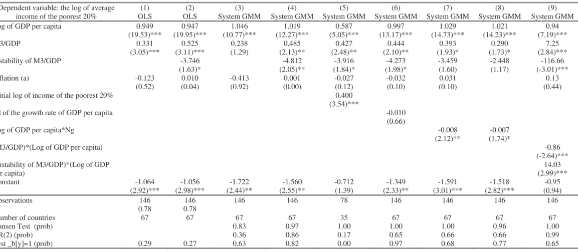
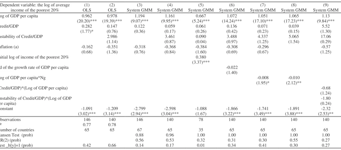
The results of the basic regression are presented in Tables I and II relative to the financial development indicators M3/GDP and Credit/GDP respectively. The first two columns show the results of OLS estimates, the subsequent columns showing the results of System GMM estimates.
In Table I, results show that the elasticity of income of the poor with respect to mean income is not significantly different from one in almost all estimates (Tables I and II), as found by Dollar and Kraay (2002). They also show that our variables of interest are significantly correlated with the mean income of the poor. The hypothesis of a positive direct effect of financial development on the standard of living of the poor is not rejected. Furthermore, financial instability significantly reduces the income of the poor.17 Financial development is more beneficial to the poor than to the average person, while the negative effect of financial instability is felt more by the poor than by the average person. Comparing column 1 to column 2 and column 3 to column 4 in Table I, it can be seen that, once we take into account the effect of financial instability on poverty, the coefficient of financial development improves in magnitude and significance. This suggests that a positive correlation exists between the instability of the financial development and its level and that, on average, financial development is more profitable to the poor in countries with a stable financial system. In addition, the positive effect of financial development on the income of the poor tends to be stronger when the country’s level of income is low while the negative effect of financial instability seems to weaken with the level of development (Column 9 of Table I). However, in Table II, the credit indicators (level and instability) are never significant, except for the private credit ratio in column 1.18 This suggests that in developing countries, the main channel of the impact of financial development on the poor is McKinnon’s “conduit effect” rather than improved access for the poor to bank credits along with the financial development
17 As the indicator of financial instability is an estimated variable, its standard error needs to be corrected. However, bootstrap estimates show that the bias is negligible.
18 The samples of Table I and II are not exactly similar, but when we run the estimations of Table I with the little smaller sample of Table II, the results are not changed.
process.19 This result is not consistent with that of Beck et al. (2004) who use the same
measure of poverty but find a significant and positive impact of private credit on the income growth of the poorest quintile of the population over twenty years. The results of this paper are probably different because our sample is composed of developing countries only while Beck et al. mixed developed and developing countries in a smaller sample (52 countries). Moreover the cross-sectional estimation of poor income growth rate is based on a longer time horizon (1960-1999) and a use of external instrumental variables.20 We remind that in Dollar and Kraay’s econometric estimation (the methodology of which is nearer of ours) financial development, measured by the ratio of commercial bank assets divide by commercial plus central bank assets, has no impact on poor income.
When McKinnon has presented the “conduit effect”, he considered money balances (currencies and demand deposits) as well as savings and time deposits, suggesting that the opportunity of accumulating money balances with a non negative real interest rate (in the absence of inflation) has a favourable impact on the investment of poor people. However, the conduit effect is reinforced when poor people have access to saving or time deposits with a positive real interest rate. Thus we have estimated the same model using the ratio of saving deposits (M3-M1) to GDP as financial indicator. The results are similar to the previous ones, with a positive coefficient of (M3-M1)/GDP which is slightly higher and a negative coefficient of its instability which is smaller.21 These results, compared with those relative to credit indicators, support the McKinnon conduit effect.
In column 5 of Tables I and II, the initial level (lagged value) of the poor’s income is introduced in order to test a convergence effect, assuming that the growth of the poor’s per capita income is all the more rapid as its initial level is low. The result concerning the effect of financial development and financial instability on poverty does not change dramatically. Financial development measured by M3/GDP still has a favourable impact on the income of the poorest, while financial instability leads to an opposite effect. In addition, the initial level is positively and significantly correlated with the current level of the dependent variable. There is evidence of a convergence effect since the coefficient of convergence (equal to the
19 This conclusion is reinforced by the fact that the interaction terms between the financial indicators and the level of per capita income are now non significant (Column 9 of Table II).
20 Legal origin of counties, absolute value of the latitude of the capital city and the religious composition of population are the instrumental variables.
initial level coefficient minus one) is negative and significant.22 However, a drawback of this
specification is a significant reduction in the sample, leading us to drop the lagged variable in the following regressions.
As regards the others explanatory variables, the inflation rate has the right sign (negative) in some columns of Tables I and II, but its coefficient lacks significance at conventional levels23. The instability of economic growth appears to be negatively correlated with the mean income of the poor when it is measured by the average income multiplied by the number of negative growth years (columns 7 and 8 of Tables I and II). In table I, the introduction of this variable reduces the marginal impact and the significance of M3/GDP instability, suggesting that the instability of economic growth is probably one of the channels of the negative effect of financial instability on the income of the poor.24
$1/day poverty rate
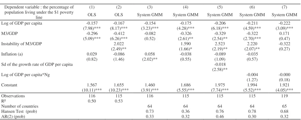
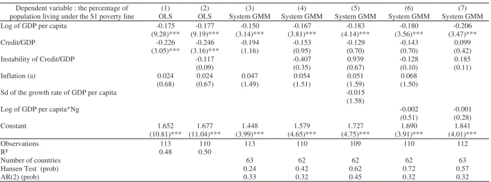
In spite of the smaller number of available observations, we run the same regressions with the second measure of monetary poverty, the share of the population below one dollar a day, used by Honohan (2004). Here we are unable to test a dynamic specification due to data limitation. The results are presented in Tables III and IV. They are similar to the previous results regarding the M3/GDP indicator.25 On the one hand, financial development is negatively associated to the headcount index while financial instability increases it (Table III). On the other hand, the significance level of the ratio of private credit to GDP improves (columns 1 and 2 of Table IV) in the OLS estimates compared to the same columns of Table II. However, its instability remains insignificant. Furthermore, neither the level nor the instability of the private credit ratio is significant in the System GMM estimates (Table IV). We may suppose that the significant impact of credit on the number of poor (most recent year available) found by Honohan (2004) in a 70 developing countries sample may be due to some problems of heterogeneity of countries in a cross-sectional estimation and of the endogeneity of explanatory variables in the absence of instrumentation.
22 For example, the coefficient of convergence in column 5 of Table I is -0.6 with a t statistic equal to -5.30. 23 It is possible that the effect of inflation is partially captured by the ratio of money to GDP which is a decreasing function of inflation.
24 To test the same hypothesis, Dollar and Kraay used an interaction term of average incomes with a dummy variable which takes the value of one when average growth is negative over the last five years; this variable was not significant when used, probably because it does not capture business cycles exactly.
25 The signs of the coefficients must be logically inverted compared to tables II and III, except for the dependant variable initial level.
An interesting result appears in the column 5 of Table III: the standard deviation of GDP per capita growth rate is significant in contrast to the other indicators of growth instability (column 6 or 7). Moreover, the coefficient is counter-intuitive. The negative coefficient of financial instability on headcount poverty may be explained by the fact that pro-poor policies are implemented in particular in countries vulnerable to exogenous shocks and with high levels of growth volatility. This result, surprisingly the inverse of that found for the average income of the poorest 20% of the population, may suggest that pro-poor policies are indeed focused on the poorest of the poor. We note that the sample average income of the poorest 20% of population is 2.2 dollars a day (see appendix 1) while the headcount index of poverty refers to an income per capita of less than one dollar a day.
Other robustness tests
Now we introduce a set of additional control variables, next to the level and instability of financial development measured by M3/GDP, in both estimations of poverty (see regressions in Tables VI and VII compared to regressions in column 4 of Tables I and III). Table VI refers to the log of average income of the first quintile as a dependent variable, while Table VII refers to the headcount index. In both tables, and as expected, the financial variables keep the right signs and remain significant in most regressions, with a significance level which is more often than not improved. To see if financial development may be regressive in the early stage of economic and financial development (in accordance with the prediction of the Greenwood and Jovanovic model, 1990), we introduce the square of M3/GDP in column 1 of Tables VI and VII, but without significant results. The same is true for several other variables, such as the inequality of land distribution or the civil liberties index. On the other hand, the instability of agricultural value added growth considered as an indirect measure of climatic shocks appears to be detrimental to the income of the poorest 20% (column 2 of Table VI) as is a high level of government consumption (columns 4 and 9 of Table VI) or trade openness (column 9 of Table VI, and column 7 of Table VII). Also, a high road density as a measure of infrastructures is positively associated with the average income of the poorest (column 8 of
Table VI),26 while a higher primary school enrolment rate appears to be negatively correlated
with the headcount index (column 9 of Table VII).
To check the potential influence of outliers we examine the residuals from the GMM estimator of our basic regression (column 4 of Tables I and III). We removed all countries with residuals more than two standard deviations away from zero and re-ran the regressions. This does not alter the results. We also used the standard deviation of the growth rate of M3/GDP as a measure of financial instability. This additional measure also suggests that financial instability is negatively and significantly (at 0.05 level) associated with the log of income of the poorest 20%, while it is positively correlated (at 0.10 level) to the headcount index.27
Economic relevance
The impacts of the level and the instability of financial development measured by M3/GDP are not only statistically significant, but also economically relevant. Concerning the specific or direct effect of financial development on the poor, a 20-percentage-point rise in M3/GDP (about one standard deviation of this ratio) would increase the average income of the poorest 20% by 9.7%, while a one standard deviation increase in the instability of M3/PIB (0.02) would lead to a 9.6% decrease in the average income of the poor (column 4 of Table I). If we now consider the headcount index, using the results in table III, we accordingly note that a 20-percentage-point increase in M3/GDP would result in a 6.5-20-percentage-point drop in the poverty rate, while a one standard deviation increase in financial instability would increase the rate of poverty by 3.18 percentage points.
In order to evaluate the total impact of financial development on poverty reduction (direct impact and indirect impact through economic growth), we should first estimate the impact of financial development and instability on economic growth. We use a standard growth model, where the growth rate of real GDP per capita is regressed on the level and the instability of financial development measured by M3/GDP, and on other usual control variables. The result obtained using System GMM estimator is presented in Table V. As expected, the level of
26 The variable road density does not have sufficient lags to allow System GMM estimation, therefore an OLS estimate is used.
financial development and its instability are respectively positively and negatively correlated to per capita GDP growth at an 0.05 significance level. We also find evidence that a high level of human capital and a reduction in black market premium, as well as low level of political instability are beneficial to economic growth.
Combining the regressions in Tables I or III and Table V, we can evaluate the total impact of financial development on the reduction of poverty, which is the sum of the direct and indirect impacts through the effect of mean income growth. A 20-percentage-point rise in M3/GDP would increase growth by 5% (Table V) and hence the average income of the poor by the same magnitude. So, the total effect of a 20-percentage-point rise in financial development would be a 14.7% rise in the income of the poorest. The total impact of a one standard deviation rise in financial instability (0.02) would be a 12.7 % drop in the average income of the poorest since the mean income would be reduced by 3.1 %. For the headcount index model (using the results in Tables III and V), the total effect of a 20-percentage-point increase in M3/GDP would be a 7.2028-percentage-point drop in the headcount index, while the total effect of a one standard deviation increase in financial instability would be 3.72-percentage-point rise in the headcount index.29
Both features of these results are to be underlined. First, it appears that financial development reduces poverty as it increases economic growth, still more by a direct effect. As it was shown previously this direct effect is probably due to a McKinnon “conduit effect”. Second, instability of financial development dramatically dampens its beneficial effect on the poor.
Conclusion
Three main results may be drawn from our analysis: (a) financial development is pro-poor; (b) financial instability hurts specifically the poor and risks to cancel the benefit of financial development; (c) in both cases a main channel of influence is probably the McKinnon “conduit effect”. Indeed, the liquidity constraint applies mainly to the investments of poor people in physical and human capital and therefore progress in financial intermediation is beneficial to the poor as it offers genuine opportunities for their savings. At
28 20*-0.326 (direct effect) + 20*0.25*-0.175 (effect through economic growth)
the same time, however, bank crises are particularly detrimental to the poor as the availability of their deposits is no longer ensured.
These conclusions may contribute to explaining the disagreements among those concerned with poverty reduction and the claim by some that growth does not help the poor. “The real debate to be engaged is on the policy package and the consequences of different elements of it for distribution and poverty” (Kanbur, 2001). The policy implications here are straightforward. As the beneficial impact of financial development on poverty reduction is dampened or even cancelled by financial instability, the policy package must take the risk of financial instability into account. Since the literature has well documented that excessive supply of money inducing inflation, large financial and trade openness in primary economies (particularly vulnerable to external shocks) and poor implementation of rule of law and international accounting standards are factors of financial crises, a policy of financial deepening should be accompanied by a stable macroeconomic framework, a progressive openness vis-à-vis the exterior and a regulation of the banking sector.
It is certainly useful to encourage the creation and the development of micro-finance especially committed to loans to the poor as credit growth does not benefit them directly. However, it is also important to control the global development of financial intermediaries as financial crises are specifically detrimental to the poor.
References
Aghion P. and P. Bolton (1997) “A Trickle-Down Theory of Growth and Development with Debt Overhang” Review of Economic Studies, vol. 64, p. 151-172
Ajewole J.O. (1989) “Some Evidence on the Demand for Money in Nigeria: A Test of the McKinnon Model of the Demand for Money in Developing Countries” Savings and
Development, vol. 13, p;183-197.
Andersen T.B. and F. Tarp (2003) “Financial Liberalization, Financial Development and Economic growth in LDCs” Journal of International Development, vol.15, n°2, p.189-209.
Arellano M. and S. Bond (1991 “Some Tests of Specification for Panel Data: Monte Carlo Evidence and an Application to Employment Equations” Review of Economic Studies, vol. 58, p. 277-297.
Arellano, M. and O. Bover (1995) “Another Look at the Instrumental-Variable Estimation of Error-Components Models”, Journal of Econometrics, vol. 68, n°1, p. 29-52.
Banerjee A. and A Newman (1993) “Occupational Choice and the Process of Development”
Journal of Political Economy, vol.101, p. 274-298.
Beck T., Demirgüç-Kunt A. and R. Levine (2004) “Finance, Inequality and Poverty: Cross-Country Evidence”, World Bank Policy Research Working Paper n° 3338.
Blundell R. and S. Bond (1998) “Initial Conditions and Moment Restrictions in Dynamic Panel Data Models” Journal of Econometrics, vol. 87, n°1, p.115-143
Bond S., Hoeffler A. and J.Temple (2001) “GMM Estimation of Empirical Growth Models” mimeo
Bruno M., Ravallion M. and L.Squire (1998) “Equity and Growth in Developing Countries: Old and New Perspectives on the Policy Issues” in V.Tanzi and K.Chu Income Distribution
and High-quality Growth, Cambridge, MA: MIT press.
Chen S. and M. Ravallion (2001), “How Did the World’s Poorest Fare in the 1990’s?” Review
of Income and wealth, vol.47, n°3, p.283-300.
Christiaensen L, Demery L. and S. Paternostra (2003) “Macro and Micro Perspectives of Growth and Poverty in Africa” The World Bank Economic Review, vol.17, n°3, p.317-347. Christopoulos D.K. and E.G. Tsionas (2004) “Financial Development and Economic Growth: Evidence from Panel Unit Root and Cointegration Tests”, Journal of Development
Deaton A. (2001) “Counting the World’s Poor: Problems and Possible Solutions”, World
Bank Research Observer, vol.16, n° 2, p.125-147.
De Melo J. and J. Tybout (1986) “The Effects of Financial Liberalization on Savings and Investment in Uruguay” Economic development and Cultural Change, vol. 34, n° 3, April, p. 561-588.
Demetriades P. and K. Hussein (1996) “Does financial development cause economic growth? Time-series evidence from 16 countries”, Journal of Development Economics, vol. 51, n° 2, p.387-411
Dollar D. and A. Kraay (2002) “Growth is Good for the Poor” Journal of Economic Growth, vol.7, n° 3, September, p.195-225.
Easterly W. (1993) “How Much Do Distortions Affect Growth” Journal of Monetary
Economics, vol.32, n° 4, p.187-212.
Easterly W. and S. Fischer (2001) “Inflation and the poor”, Journal of Money, Credit and
Banking, vol.33, n° 2, p.160-178.
Edwards S. (1988) “Financial Deregulation and segmented Capital Market: The Case of Korea” World Development, vol.16, p. 185-194.
Fry M. J. (1978) “Money and Capital or Financial Deepening in Economic Development”
Journal of Money, Credit and Banking” vol.10, November, p. 464-475.
Fry M. J. (1988) Money, Interest and Banking in Economic Development, Baltimore: Johns Hopkins University Press.
Gertler M. and A. Rose (1994) “Finance, Public Policy and Growth” in G. Caprio, I. Atiyas and J. Hanson (eds), Financial Reform: Theory and Experience, New-York, Cambridge University Press, p.13-14.
Greenwood J. and B. Jovanovic (1990) “Financial Development, Growth and the Distribution of Income” Journal of Political Economy, vol.98, n°5, October, p.1076-1108.
Guillaumont P., Guillaumont Jeanneney S. and J-F Brun (1999) “How Instability Lowers African Growth” Journal of African Economies, vol.8, n°1, p.87-107.
Gurley J.G. and E.S. Shaw (1960) Money in a Theory of Finance, Brookings Institution, Washington D.C.
Honohan P. (2004) “Financial Development, Growth and Poverty: How Close Are the Links?” World Bank Policy Research Working Paper 3203, February.
Jalilian and Kirkpatrick (2002) “Financial Development and Poverty Reduction in Developing Countries” International Journal of Finance and Economics, vol.7, n°2, p.97-108
Janvry (de) A. and E. Sadoulet (2000) “Growth, Poverty, and Inequality in Latin America: A Causal Analysis, 1970-1994” Review of Income and Wealth, vol. 46, n°3, September, p.267-287.
Kanbur R. (2001) “Economic Policy, Distribution and Poverty: The Nature of the Disagreements” World Development, vol.29,n°8, p.1083-1094.
Kar M. and E.J. Pentecost (2001) “A System Test of McKinnon’s Complementary Hypothesis With an Application to Turkey” mimeo, february.
Kaufmann D., Kraay A. and P. Zoido-Lobatón (2002) “Governance Matters II: Updated Indicators for 2000/01”, mimeo, The World Bank.
Keynes J.M. (1937) “The ex ante Theory of the Rate of Interest” The Economic Journal, December, and The General Theory and After, Part II Defence and Development, Macmillan for the Royal Society, p. 215- 223.
Khan A.H. and L. Hasan (1998) “Financial Liberalization, Savings, and Economic Development in Pakistan” Economic Development and cultural change, Vol.46, n°3, April, p. 581-598.
Khan M.S. and A.S. Senhadji (2003) “Financial Development and Economic Growth”
Journal of African Economies, vol.12, suppl.2, p.89-110.
King G. and R. Levine (1993) “Finance and Growth: Schumpeter Might Be Right?” The
Quarterly Journal of Economics, vol. 108, n°3, p.1076-1107
Laumas P.S. (1990) “Monetization, Financial Liberalization and Development” Economic
Development and cultural change, vol 38, January,p. 377-390.
Levine R. (1997) “Financial Development and economic Growth: Views and Agenda”
Journal of Economic Literature, vol. 35, n°3, June, p.688-726.
Levine R., Loayza N. and T. Beck (2000) “Financial Intermediation and Growth: Causality and Causes” Journal of Monetary Economics, vol. 46, n° 1, august, p.31-77.
Loayza N. and R. Ranciere (2002) “Financial Development, Financial Instability, and Growth” CESifo Working Paper n°684.
Lundberg M. and L. Squire (2003) “The Simultaneous Evolutions of Growth and Inequality”
The Economic Journal, vol.113, Issue 487, p. 326-344.
McKinnon R.I. (1973) Money and Capital in Economic Development, Washington, The Brooking Institution.
Morriset J. (1993) “Does Financial Liberalisation Really Improve Private Investment in Developing Countries?” Journal of Development Economics, vol. 40 p.133-150.
Mosley P. (1999) “Micro-macro Linkages in Financial Markets: The Impact of Financial Liberalisation on Access to Rural Credit in Four African Countries” Journal of International
Pagano M. (1993) “Financial Markets and Growth: an Overview” European Economic
Review, vol.37, n°2-3, p.613-622.
Rajan R. and L. Zingales (2003) “The Great Reversals: the Politics of Financial Development in the 20th Century” Journal of Financial Economics, vol.69, p.5–50
Ram R. (1999) “Financial development and economic growth: additional evidence”, Journal
of Development Studies, vol. 35, n°4, p.164–174.
Ramey G. and V.A Ramey (1995) “Cross-country Evidence on the Link Between Volatility and growth” The American Economic Review, vol. 85, n° 5, December, p.1138-1151.
Ravallion M. (2001) “Growth, Inequality and Poverty: Looking Beyond Averages” World
Development, vol. 29, n°11, p.1803-1815
Roubini N. and X. Sala-i-Martin (1992) “Financial Repression and Economic Growth”
Journal of Development Economics, vol.39, n°1, January, p.5-30.
Thornton J. and S.R. Poudyal (1990) “Money and Capital in Economic Development: A Test of the McKinnon Hypothesis for Nepal” Journal of Money, Credit and Banking, vol. 22, august 1990, p. 395-399.
APPENDIX I: Descriptive statistics
Sample of 75 developing countries for which the income of
the poorest 20% is available (1966-2000) Sample of 65 developing countries for which the headcount index is available (1980-2000) Variable Observations Mean deviation Minimum Maximum Standard Observations Mean Standard deviation Minimum Maximum
Mean income of the poorest 20% 187 670 502 42 2882
GDP per capita (constant 1985 USD at PPP) 187 2461 1871 329 11738
Headcount index 121 0.258 0.214 0.001 0.823
GDP per capita (constant 1993 USD at PPP) 120 2881 2043 440 9920
M3/GDP 187 0.365 0.214 0.073 1.419 121 0.355 0.190 0.115 1.294
Instability of M3/GDP 187 0.023 0.018 0.004 0.126 120 0.027 0.027 0.004 0.183
Credit/GDP 166 0.210 0.164 0.012 0.993 116 0.203 0.151 0.014 0.745
Instability of Credit/GDP 153 0.016 0.012 0.004 0.076 113 0.017 0.012 0.000 0.059
Inflation rate 155 0.207 0.258 -0.040 1.727 116 0.398 1.337 0.006 12.642
sd of agricultural value added (%of GDP)
growth* 182 8.182 7.342 0.454 50.616 119 8.428 7.414 0.000 50.616
sd of GDP per capita growth* 187 3.502 2.258 0.425 12.535 120 3.301 2.150 0.288 11.567
Gini index of land distribution 144 66.52 16.59 31.21 93.31 91 66.71 16.98 31.77 93.31
Primary school enrolment rate (Education) 170 0.927 0.231 0.245 1.376 120 0.915 0.251 0.245 1.341
Civil liberties index 162 2.872 1.305 0 6 121 2.864 1.294 0 6
Road density 73 0.240 0.346 0.007 1.581 85 0.269 0.398 0.007 1.660
Trade openness (%) 184 57.67 32.23 8.17 181.82 120 58.22 28.93 9.50 137.91
Government consumption/GDP 184 0.130 0.051 0.044 0.318 120 0.131 0.049 0.046 0.295
APPENDIX II: Variables and Sources
Variable Definition Source of data
Log of income of the poorest 20% Log of average incomes in bottom quintile, constant 1985 USD at PPP Dollar and Kraay (2002) Log of GDP per capita (1985 PPP) Log of average per capita income, 1985 USD at PPP Dollar and Kraay (2002)
Headcount index The percentage of the population living below the $1/day international poverty line http://www.worldbank.org/research/povmonitor World Bank Global Poverty Index Database Log of GDP per capita PPP Log of GDP per capita based on purchasing power parity (PPP) World Development Indicators 2003
M3/GDP Liquid liabilities as a percentage of GDP World Development Indicators 2003
Instability of M3/GDP regressed on its lagged level and a trend over the Standard deviation of the residuals of M3/GDP
period 1966-2000 World Development Indicators 2003
Credit/GDP Private credit by deposit money banks to GDP Financial Structure Database 2001 The World Bank
Instability of Credit/GDP Credit/GDP regressed on its lagged level and a Standard deviation of the residuals of trend over the period 1966-2000
Financial Structure Database 2001 The World Bank
Inflation rate Growth of consumer price index World Development Indicators 2003
Agricultural value added Agricultural value added as a share of GDP World Development Indicators 2003
GDP per capita growth Growth of real GDP per capita World Development Indicators 2003
Gini index of land distribution Land distribution inequality (Data are average from 1950 to 1990) Lundberg and Squire (2003)
Education Primary school enrolment rate World Development Indicators 2003
Civil liberties index
Civil liberties are measured on a one-to-seven scale, with one representing the highest degree of freedom and seven the lowest. To facilitate interpretation of this variable, we use 7 minus
the index civil liberties in the regressions
Freedom House Database 1999
Road density The ratio of total road network (km) to the total area of the country (square km) World Development Indicators 2003
Government consumption/GDP Government expenditure as share of GDP World Development Indicators 2003
Political instability Number of riots, attacks, strikes and coup d'état CERDI database (2000)
Black market premium The percentage difference between the black market rate and the official exchange rate Global Development Network Database (1999)
Trade openness Sum of real exports and imports as share of GDP Penn World Table 6.1
Table I: Financial development (M3/GDP), financial instability and poverty (The log of average income of the poorest 20%)
Absolute value of robust t statistics in brackets
* significant at 10%; ** significant at 5%; *** significant at 1% AR(2) : Arellano and Bond test of second order autocorrelation
Test _b[y] =1: tests the Ho assumption such that the coefficient of the log of GDP per capita is not different from one Ng= Number of negative growth during five years (the year of poverty measurement and the four preceding years) Sd : standard deviation
(a) Log (1+ inflation rate)
(1) (2) (3) (4) (5) (6) (7) (8) (9)
Dependent variable: the log of average
income of the poorest 20% OLS OLS System GMM System GMM System GMM System GMM System GMM System GMM System GMM
Log of GDP per capita 0.949 0.947 1.046 1.019 0.587 0.997 1.029 1.021 0.94
(19.53)*** (19.95)*** (10.77)*** (12.27)*** (5.05)*** (13.17)*** (14.73)*** (14.23)*** (7.19)*** M3/GDP 0.331 0.525 0.238 0.485 0.427 0.444 0.393 0.290 7.25 (3.05)*** (3.11)*** (1.29) (2.13)** (2.48)** (2.10)** (1.93)* (1.73)* (2.84)*** Instability of M3/GDP -3.746 -4.812 -3.916 -4.273 -3.459 -2.448 -116.66 (1.63)* (2.05)** (1.84)* (1.98)* (1.60) (1.17) (-3.01)*** Inflation (a) -0.123 0.010 -0.413 0.001 -0.027 -0.032 0.031 0.13 (0.52) (0.04) (0.92) (0.00) (0.12) (0.10) (0.10) (0.44)
Initial log of income of the poorest 20% 0.400
(3.54)***
Sd of the growth rate of GDP per capita -0.010
(0.66)
Log of GDP per capita*Ng -0.008 -0.007
(2.12)** (1.74)*
(M3/GDP)*(Log of GDP per capita) -0.86
(-2.64)*** (Instability of M3/GDP)*(Log of GDP 14.03 per capita) (2.99)*** Constant -1.064 -1.056 -1.722 -1.560 -0.712 -1.349 -1.591 -1.518 -0.95 (2.92)*** (2.98)*** (2.44)** (2.55)** (1.39) (2.33)** (3.01)*** (2.82)*** (0.94) Observations 146 146 146 146 78 146 146 146 146 R² 0.78 0.78 Number of countries 67 67 67 67 35 67 67 67 67
Hansen Test (prob) 0.83 0.97 1.00 1.00 1.00 0.96 1.00
AR(2) (prob) 0.36 0.86 0.17 0.65 0.66 0.66 0.99
Table II: Financial development (Credit/GDP), financial instability and poverty (The log of average income of the poorest 20%)
Absolute value of robust t statistics in brackets
* significant at 10%; ** significant at 5%; *** significant at 1% AR(2) : Arellano and Bond test of second order autocorrelation
Test _b[y] =1: tests the Ho assumption such that the coefficient of the log of GDP per capita is not different from one Ng= Number of negative growth during five years (the year of poverty measurement and the four preceding years) Sd : standard deviation
(a) Log (1+ inflation rate)
All explanatory variables are assumed to be predetermined
(1) (2) (3) (4) (5) (6) (7) (8) (9)
Dependent variable: the log of average
income of the poorest 20% OLS OLS System GMM System GMM System GMM System GMM System GMM System GMM System GMM
Log of GDP per capita 0.962 0.978 1.194 1.161 0.667 1.072 1.051 1.065 1.13
(20.20)*** (19.39)*** (9.07)*** (9.95)*** (5.24)*** (14.24)*** (17.10)*** (17.23)*** (9.84)*** Credit/GDP 0.282 0.147 0.122 0.059 0.061 0.136 0.071 0.039 5.52 (1.77)* (0.76) (0.36) (0.17) (0.26) (0.42) (0.23) (0.15) (1.30) Instability of Credit/GDP 2.986 3.461 0.090 3.488 4.337 5.065 17.06 (1.14) (0.87) (0.04) (0.97) (1.25) (1.54) (0.29) Inflation (a) -0.162 -0.351 -0.318 -0.368 -0.384 -0.308 -0.296 -0.57 (0.68) (1.36) (0.76) (0.84) (1.60) (0.69) (0.67) (1.25)
Initial log of income of the poorest 20% 0.380
(3.37)***
Sd of the growth rate of GDP per capita -0.022
(1.40)
Log of GDP per capita*Ng -0.008 -0.010
(1.95)* (2.12)**
(Credit/GDP)*(Log of GDP per capita) -0.68
(1.24) (Instability of Credit/GDP)*(Log of GDP -1.80 per capita) (0.24) Constant -1.091 -1.209 -2.799 -2.598 -1.088 -1.866 -1.741 -1.891 -2.32 (3.02)*** (3.14)*** (2.94)*** (3.04)*** (1.67) (3.22)*** (3.49)*** (3.88)*** (2.53)** Observations 146 140 146 140 78 140 140 140 140 R² 0.77 0.78 Number of countries 65 65 67 65 35 65 65 65 65
Hansen Test (prob) 0.88 0.96 1.00 1.00 1.00 1.00 1.00
AR(2) (prob) 0.56 0.53 0.32 0.31 0.30 0.55 0.27
Table III: Financial development (M3/GDP), financial instability and poverty (headcount index)
Absolute value of robust t statistics in brackets
* significant at 10%; ** significant at 5%; *** significant at 1% AR(2) : Arellano and Bond test of second order autocorrelation
Test _b[y] =1: tests the Ho assumption such that the coefficient of the log of GDP per capita is not different from one Ng= Number of negative growth during five years (the year of poverty measurement and the four preceding years) Sd : standard deviation
(a) Log (1+ inflation rate)
All explanatory variables are assumed to be predetermined
(1) (2) (3) (4) (5) (6) (7)
Dependent variable : the percentage of population living under the $1 poverty
line OLS OLS System GMM System GMM System GMM System GMM System GMM
Log of GDP per capita -0.157 -0.167 -0.154 -0.175 -0.206 -0.211 -0.222
(7.98)*** (8.17)*** (3.23)*** (4.28)*** (6.18)*** (4.59)*** (3.09)*** M3/GDP -0.296 -0.412 -0.082 -0.326 -0.329 -0.322 0.171 (5.09)*** (6.26)*** (0.52) (2.61)** (2.54)** (2.70)*** (0.47) Instability of M3/GDP 2.022 1.590 2.523 2.220 -0.322 (2.49)** (1.66)* (2.19)** (2.07)** (0.27) Inflation (a) 0.029 -0.086 0.058 -0.038 -0.089 -0.035 (0.82) (1.46) (2.02)** (0.55) (1.09) (0.57)
Sd of the growth rate of GDP per capita -0.018
(2.58)**
Log of GDP per capita*Ng -0.004 -0.000
(1.27) (0.18) Constant 1.567 1.655 1.460 1.686 1.975 1.994 1.921 (10.11)*** (10.23)*** (3.91)*** (5.55)*** (7.74)*** (5.52)*** (4.05)*** Observations 116 115 116 115 115 115 119 R² 0.50 0.53 Number of countries 64 64 64 64 65
Hansen Test (prob) 0.73 0.36 0.76 0.78 0.68