HAL Id: halshs-01402997
https://halshs.archives-ouvertes.fr/halshs-01402997
Preprint submitted on 25 Nov 2016HAL is a multi-disciplinary open access archive for the deposit and dissemination of sci-entific research documents, whether they are pub-lished or not. The documents may come from teaching and research institutions in France or abroad, or from public or private research centers.
L’archive ouverte pluridisciplinaire HAL, est destinée au dépôt et à la diffusion de documents scientifiques de niveau recherche, publiés ou non, émanant des établissements d’enseignement et de recherche français ou étrangers, des laboratoires publics ou privés.
Do Inequality and Institutions Matter?
Aïssata Coulibaly
To cite this version:
Aïssata Coulibaly. Revisiting the Relationship between Financial Development and Child Labor in Developing Countries: Do Inequality and Institutions Matter?. 2016. �halshs-01402997�
SÉRIE ÉTUDES ET DOCUMENTS
Revisiting the Relationship between Financial Development
and Child Labor in Developing Countries: Do Inequality and
Institutions Matter?
Aïssata Coulibaly
Études et Documents n° 19
November 2016To cite this document:
Coulibaly A. (2016) “Revisiting the Relationship between Financial Development and Child Labor in Developing Countries: Do Inequality and Institutions Matter?”, Études et Documents, n°19 , CERDI. http://cerdi.org/production/show/id/1831/type_production_id/1
CERDI
65 BD. F. MITTERRAND
63000 CLERMONT FERRAND – FRANCE TEL.+33473177400
FAX +33473177428
2
The author
Aïssata Coulibaly
PhD Student in Economics
CERDI – Clermont Université, Université d’Auvergne, UMR CNRS 6587, 65 Bd F. Mitterrand, 63009 Clermont-Ferrand, France.
E-mail: [email protected]
This work was supported by the LABEX IDGM+ (ANR-10-LABX-14-01) within the program “Investissements d’Avenir” operated by the French National Research Agency (ANR).
Études et Documents are available online at: http://www.cerdi.org/ed
Director of Publication: Vianney Dequiedt Editor: Catherine Araujo Bonjean
Publisher: Mariannick Cornec ISSN: 2114 - 7957
Disclaimer:
Études et Documents is a working papers series. Working Papers are not refereed, they constitute research in progress. Responsibility for the contents and opinions expressed in the working papers rests solely with the authors. Comments and suggestions are welcome and should be addressed to the authors.
3
Abstract
This paper analyzes the relationship between financial development and child labor for a panel of developing countries over the period 1960 to 2004. We find that financial development measured by the ratio of private credit to GDP tends to increase child labor and this result is driven by countries with high level of inequality, above to the mean of the Gini coefficient. This could reflect that with access to credit, households tend to invest in their own farm or family business, raising the opportunity cost of schooling and inducing more working children. These findings are robust to the use of different estimation techniques like instrumental variables strategy and generalized method of moments. But this positive effect is likely to be non nonlinear, especially financial development and education spending are effective in reducing child labor only in countries with better control of corruption. This suggests that better institutions by improving the quality of education services and its return tend to alter the positive impact of financial development which occurs via the high opportunity cost of education.
Keywords
Child labor, Financial development, Institutions, Inequality, SWIID.
JEL Codes
4
1. Introduction
Despite many efforts from governments and the international community, child labor is still prevalent in many developing countries. According to the last estimates of the International Labor Organization (ILO), in 2013, about 11% of the world’s child population between the ages of 5 and 17 years old were concerned by child labor in 2012, accounting for 168 million of children. Regarding its negative consequences on children human capital development and their prospects for adulthood, this topic is at the core of development studies. So, a wide range of articles have investigated the determinants of child labor both theoretically and empirically and it comes out that poverty is likely the main driving factor. Nevertheless, this finding is challenged by recent micro-studies. For instance landholding, a strong predictor of income level in developing countries, has been found to be associated with more child labor1 with children working on farms operated by their families as in Ghana and Pakistan (Bhalotra & Heady 2003) or in Burkina-Faso (Dumas 2006). For Dumas (2013), this “wealth paradox” could be explained by labor and credit market imperfections, suggesting the importance of other factors beyond growth and absolute poverty.
This article revisits the link between credit markets imperfections and child labor for a panel of developing countries from 1960 to 2004. Major empirical studies on this topic at macroeconomic level are those of (Dehejia & Gatti 2005; Ebeke 2012). They find that child labor is associated negatively to financial development measured by private credit ratio. In this formulation, access to credit prevent households to use child labor in order to smooth their consumption in case of shocks. The main limit of these studies is that they do not take into account time dimension in the data. For instance, the study by Ebeke (2012) focuses only on the year 2000 due to data availability for migration. While, Dehejia and Gatti (2005), in their identification strategy, use as instruments for financial development, the rate of mortality among colonial settlers and the origin of legal systems which do not vary across time. Moreover their negative finding is questioned by some microeconomic studies (e.g, (Wydick 1999; Menon 2010; Hazarika & Sarangi 2008) ). These studies emphasized that a better access to credit can increase child labor, especially if parents invest in productive activities like expanding the family business
1
This is the “wealth paradox” meaning that children from rich families are engaged in work in their family business or farm.
5
or farm. This can raise the returns from child labor especially if labor markets are imperfect due to shortages in hiring or to moral hazard. In this case, parents are more confident in the workforce of their own children as the opportunity cost of education has increased.
In addition, a recent literature has highlighted a relationship between financial development and inequality, which has been neglected by previous studies looking at the impact of access to financial services on child labor. Indeed, we argue that child labor is more prevalent in presence of inequalities as demonstrated by (Tanaka 2003; D’Alessandro & Fioroni 2016; Ranjan 2001)2. In this case, financial development which increases (decreases) inequality can also lead to more (less) child labor indirectly.
The literature on the relationship between financial development and inequality could be divided in two strands: linear vs. non-linear approaches. On the one hand, the advocates of the linear hypothesis argue that financial development can increase or reduce inequalities depending on who benefit from better access to financial services. If financial development benefits the rich because they can afford for collateral and are more able to repay a loan, it is the inequality widening hypothesis where the poor continue to be excluded (Rajan & Zingales 2003). On the contrary, it is the inequality narrowing hypothesis with better access to credit or insurance for the poor (Beck and al. (2007); (Mookerjee and Kalipioni 2010)). In the other and, some authors highlight a non-linear relationship between inequality and financial development. Greenwood and Jovanovic (1990) refer this as an inverted U relationship between the two variables. This suggests that below a critical point of financial development, the poor are hurt and this exacerbates inequality as demonstrated by Kim and Lin (2011). But, Tan and Law (2012) find an U-shape relationship between inequality and financial development for a panel of 35 developing countries, suggesting that even if at earlier stages of development, poor can benefit from better developed credit markets. Law and al. (2014) also emphasizes that this non-linear relationship is correlated with the level of institutional quality. They find that financial development decreases inequality only beyond a certain level of institutional quality.
Consequently, this paper aims to study empirically the impact of financial development on child labor while controlling for the level of inequality. Our contribution is fourfold: (1) we exploit the time dimension of the data for child labor which allow us to have more variability compared to previous macroeconomic studies. (2) We try to conciliate diverging results between
6
studies whose find a negative impact of financial development at macroeconomic level to those who find a positive effect at microeconomic level, our intuition is that the different impact of financial development on child labor could be linked to the persistence of inequality. (3) We also propose an identification strategy to deal with the endogeneity of financial development. We build upon the existing literature to find an exogenous source of variation. We argue that credit information sharing is expected to have an impact on the development of the financial sector as it allows to have information about borrowers’ discipline and limits information asymmetry with the lender. Especially, like Ebeke (2012), we use as instrument for financial development, the existence of public credit bureau and private credit registries. They maintain a database on the standing of borrowers in the financial system and facilitate the exchange of information amongst banks and financial institutions without influencing directly child labor. (4) We investigate whether the effect of financial development on child labor is nonlinear by looking at conditional effects linked to the level of inequality and the quality of institutions.
We find a positive correlation between financial development, measured by the ratio of private credit to GDP, and child labor especially when inequalities are high, above the mean for our measure of inequality, below the mean we find that financial development tend to reduce child labor. Our results are robust to the use of other estimation techniques like instrumental variables strategy and generalized methods of moments. Many explanations are possible for the positive effect of financial development. Based on our literature review, on the one hand, they can emphasize that credit is used in productive activities which raise the demand for child labor by boosting local economy. On the other hand, it could reflect that households tend to invest in their own farm or business. This raises the opportunity cost of schooling and induce more working children. Especially in sectors that necessitate a great supervision and where risk of moral hazards from hired labor is important, In this case, parents would prefer to rely on the workforce of their own children, even though credit constraints are no more binding. These findings are similar to those of Menon (2010), and Hazarika and Sarangi (2008).
Given this positive effect of financial development, we also test the idea that improving educational quality through better governance could help reduce child labor. Our intuition is that parents in their choice of sending their children to work or not, would confront the high opportunity cost of education to the returns from education. In fact, parents’ decision depends on essentially three things: the cost (including the opportunity-cost) of education, the expected return
7
to education, and the extent to which they are able to finance educational investments (Cigno et al. 2002). Especially, households would rationally prefer child labor if the high opportunity cost of education is associated to a lower marginal benefit from schooling. Consequently, we argue that policies which tend to improve the quality of education raising its return can reduce child labor, this could be done through better bureaucracy quality and fewer corruption. To test this hypothesis, we introduce an interaction term between private credit ratio and indicators of the quality of institutions. We also test directly the impact of the provision of education services and their quality by introducing as additional controls; education spending to GDP, and the survival rate from grade five of primary education which measures the share of children enrolled in the first grade of primary school who eventually reach grade five.
Our results suggest that financial development and education spending will be effective in reducing child labor only in countries with better control of corruption which improves the provision of public services and raises its marginal benefit. Moreover, a higher survival rate which is associated to a more efficient education system tends to reduce child labor. This adds more evidence to our intuition that a better quality of education is likely to limit the positive impact of a higher opportunity cost of education on child labor.
The remainder of the paper is organized as follows, after revisiting the last findings on the relationship between financial development, inequality and child labor, we present our analytical framework in section 2. Section 3 is devoted to our empirical strategy while in section 4, we discuss our results with some robustness check then we conclude in Section 5.
2. Literature review
2.1.
Financial development and child labor
According to the theoretical model developed by Ranjan (2001), child labor occurs because of credits constraints and inequality so a policy which limits them through access to financial services or redistribution may reduce it. Many lessons can be drawn from empirical studies aimed at studying the impact of financial development on child labor. Firstly, the negative impact of financial development on child labor is observed generally when credits constrained household rely on child labor to smooth their income in case of shocks. For example, inflation can lead to
8
more child labor used to compensate the reduction of the purchasing power of the poorest household, as they are the more hurt by this situation. In fact, price instability can hurt the poor and the middle class more than the rich. Firstly, because the latter have better access to financial instruments that allow them to hedge their exposure to inflation (Easterly & Fischer 2001). Secondly, the poor pay a disproportionate share of the inflation tax as they hold more cash relative to other financial assets (Erosa & Ventura 2002). This has been verified in micro-studies, independently of the nature of the shock whether it is idiosyncratic, specific to the household (Guarcello et al. 2010) or common (Alvi & Dendir 2011) like floods or drought. At macro-level, using data on private credit ratio to GDP; Dehejia and Gatti (2005) or Ebeke (2012) also emphasize that the main transmission channel through which financial development exerts an effect on child labor at cross country level is income volatility.
On the other hand, within the framework of micro-studies, some authors have demonstrated that access to credit can increase child labor especially if it is used to invest in productive activities like family farm or non-farm enterprises which increases the opportunity cost of schooling and induce more working children. Especially, Wydick (1999) highlights that parents after investing in their family business or firm can prefer to hire their children, because investment in capital raises the opportunity cost of schooling and increases labor productivity at household level. Moreover, in sectors that necessitate a great supervision and where risk of moral hazards from hired labor is important, parents would prefer to rely on the workforce of their own children, even though credit constraints are no more binding. These findings are similar to those of Menon (2010), and Hazarika and Sarangi (2008). So, the effect of financial development on child labor is not predetermined and at household level, it is driven by different factors linked to the context, the use of credits and household characteristics.
2.2.
Inequality and child labor
The relationship between inequality and child labor has been less investigated both theoretically and empirically with a focus on poverty and growth. First, at macro-level, empirical studies suggested that child labor is associated negatively with income growth but these results have been challenged by micro-studies with mixed results. In some cases income growth may not result in the decrease of child labor, due to the persistence of inequality despite growth ( e.g.
9
Sarkar and Sarkar (2012)). In fact, unequal distribution of income due to gaps in productivity or skills between households ( e.g. Basu and Van (1998) and (1999), Rogers and Swinnerton (1999) and (2001), Dessy and Vencatachellum (2003) ) have been demonstrated to explain child labor phenomenon. For Emerson and Knabb (2006), we must go beyond income inequality which could be explained by unequal access to opportunities. As opportunity, he refers to school quality, access to higher paid jobs, access to information about the returns to education and actual discrimination, so treating these causes could help reduce child labor
At theoretical level, Basu and Van (1998) develop a model where child labor depends on whether adult income is below or above some subsistence level. If the economy is sufficiently productive, wages are high enough to ensure that all households are above the subsistence level and send their children to school, then there is no child labor (good equilibrium). Nevertheless if wages are low, children are sent to work (bad equilibrium). Swinnerton and Rogers (1999) extend this model to introduce the proportion “α” of firms’ benefits which are distributed to households. They conclude that if all workers in the economy receive dividends, the “bad equilibrium” where children have to work does not exist. Hence, they propose a policy that redistributes dividends across workers as a way of eliminating the “bad equilibrium”. Basu and Van (1999) reply to this comment by allowing “α” to fluctuate between 0 and 1 (α ϵ [0,1] ); α = 0 leads to Basu and Van (1998) conclusion with only a bad equilibrium where all children work. If α = 1, the model corresponds to Swinnerton and Rogers (1999) with no child labor (good equilibrium). But if α is not equal to zero but inferior to 1, we have an hybrid equilibrium with some children going to school and other working, this is closer to the current situation in developing countries. In order to respond to the precedent-study of Basu and Van (1999), Rogers and Swinnerton (2001) develop a theoretical model to take into account the role productivity plays in determining the effects of a reduction of income inequality on child labor. They find that decreasing inequalities through a redistributive tax can increase child labor. Especially in poor countries with low productivity, redistribution may not be sufficient to bring the poorest households out of poverty and the tax burden supported by households at the margin of subsistence3 could be so important that they have to send their children to work. But Ranjan (2001) develops a dynamic theoretical model where he emphasizes that with such a transfer, the increase in the probability of sending
3
Households for which an important taxation pushes them below the subsistence level of income so that they are obliged to send their children to work.
10
the child to work for a rich person is lesser than the decrease in the probability of sending the child to work for the poor, so we can expect a positive association between child labor and inequality. Moreover, he emphasizes that in the precedent studies, inequality is measured by the proportion of households who receive dividends which are equally distributed among them. In its model, inequality refers to the distribution of total parental income and is modelled in the sense of a second order stochastic dominance (Lorenz dominance for distributions with same mean). He finds that for a same level of income, distributions with higher level of inequality would result in more child labor at the equilibrium. In the same vein, Tanaka (2003) develops a theoretical model in which unequal distribution of income could also lead to child labor. He considers that for a given level of income, if the median income is below a certain threshold level, public schooling is no more supported by the majority of households4 who do not want to support more taxation and / or lose a source of income with their children going to school, reducing both the supply and the demand for education. As implication, redistribution policies that increase the median income above this threshold will result in more school attendance and less child labor
Likewise, D’Alessandro & Fioroni (2016) develop a theoretical model where they distinguish between unskilled parents who tend to have a high number of children and send them to work and skilled parents who have a low fertility rate with a high investment in education. The fertility differential between high and low skilled increases the proportion of unskilled workers in the labor market which in turns reduces unskilled wages. So, the fact that children can offers only unskilled labor reinforces such process creating a vicious cycle between child labor and inequality.
The positive link between inequality and child labor is also confirmed by empirical studies. At country level, Nawaz et al. (2011) also demonstrate that for Pakistan, inequality has a positive and significant impact on child labor in the long term while the negative association between school attendance and inequality is confirmed by Checchi (2003) for a panel of 108 countries over the period 1960–1995. Our study is complementary to this paper, because as underlined by Ravallion and Wodon (2000) with data from Bangladesh, schooling and child labor are not necessarily one-for-one substitutes.
4
He demonstrates that for a given income per capita Y, “if the economy has income distribution with low median income, the economy ends up with an enormous amount of child labor. However, if the income distribution of the economy has high median income, the amount of child labor falls significantly” (Tanaka, 2003 page 97).
11
2.3.
Financial Development and Inequality
A recent literature has emphasized the distributional impact of financial development on income. Financial development could reduce poverty and inequality by allowing the poor more than the rich to finance their project or smooth their income (Beck, Demirgüç-Kunt, et al. 2007). But a better access to credit or financial services is not automatically a pro-poor issue. Other studies have demonstrated that the poor can be excluded from the benefits of financial system because they generally lack collateral, credit histories and connection. Thus, this increases inequalities given that the rich are more likely to take advantage from financial development. Greenwood and Jovanovic (1990) highlight that this situation is verified only at early stages of development. For them, the relation is non-linear and take the form of an inverted – U relationship. It is after a certain level of growth that the poor constitute a capital which allow them to participate to the financial system. But, Tan and Law (2012) emphasize the contrary with a U-shape relationship, for them, it is after a certain level of development that financial development increases inequality, below that level, it is reduced, with more profit for to the poor. Furthermore, in developing countries with weak institutional quality, lack of check and balances, income inequality could also be translated on unequal access to finance where elites can prevent the poor from benefiting to financial access through direct control or regulatory capture of the financial system (e.g. Rajan and Zingales (2003); Claessens and Perotti (2007)). It is the case when, for example, connecting firms are favored in access to credit in order to maintain the privileges and the political power of the ruling class. The latter is against diffusion of education which promotes political participation and weakens control structures (Bourguignon & Verdier 2000). These authors also emphasize that the poor rely more on informal networks for credit, so financial development would only benefit the rich and raise inequality.
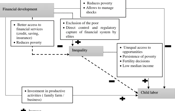
Subsequently, given the relationship between inequality and financial development, it seems relevant to check if differences on the effect of financial development on child labor are not linked with distributional issues. In figure 1 below, we present an overview of the different relationship between child labor, financial development and inequality based on our literature review, continuous lines are for direct relations and discontinuous lines for indirect connections. First, financial development has a direct negative impact on child labor by allowing poor people to have access to credit and invest in their children education. They are also able to manage shocks and do not use child labor as a smoothing mechanism. But financial development can also
12
increase child labor if credit is used to invest in productive activities like family farm or non-farm enterprises which increase the opportunity cost of schooling and induce more working children. Moreover we have an indirect link through inequality, under the assumption that child labor is more prevalent when inequalities are high, financial development could increase child labor if it
raises inequality and vice versa.
Figure 1: Links between financial development, inequality and child labor
Source: author’s compilation
3. Empirical Model
Previous studies looking at the impact of financial development on child labor do not pay attention to its redistributive effects on income which have been emphasized by recent studies. The object of this article is to study how the links between inequality and financial development may explain cross country panel variation of child labor.
Financial development
Inequality
Child labor
Investment in productive activities ( family farm / business)
Exclusion of the poor
Direct control and regulatory capture of financial system by elites Better access to financial services (credit, saving, insurance) Reduces poverty Reduces poverty Allows to manage shocks Unequal access to opportunities Persistence of poverty Fertility decisions
Low median income
Increase Decrease
13
Based on the literature on child labor at macroeconomic level ( e.g. Dehejia and Gatti (2005), Kis-Katos (2007); Ebeke (2012)), we specify the following equations :
Model 1: Clit = α + β X’it+ δFDit + µi +vt + εit (1)
Model 2: Clit = α + β X’it+ δFDit + γIit + µi +vt + εit (2)
In equation (1) , Clit , FDit, µi, vt, and εit represent respectively the prevalence of child
labor, private credit ratio, country fixed effects, time effect of period t and the error term in country i at year t. The vector X’ contains the traditional determinants of child labor in macroeconomic studies. Thus, we include GDP per capita and its square, percentage of rural population, share of agriculture value added in GDP, trade openness measured by the logarithm of the ratio of exports plus imports to GDP and a variable equal to 1 since a country has adopted the ILO convention 138 establishing minimum working ages. In equation (2), we introduce Inequality (Iit), in order to assess the effect of private credit ratio while controlling for inequality.
We expect the coefficients for rural population, share of agriculture in GDP, and inequality to be positive following the results of previous works ( e.g. Edmonds and Pavcnik (2006), Davies and Voy (2009), Dehejia and Gatti (2005) and Ebeke (2012)). We suppose that trade openness may reduce child labor prevalence like Kis-Katos (2007).
We also allow for the log of income per capita to enter the specification nonlinearly because the effects of income on child labor likely differ across poor and rich countries. For each country, the relation will depend on whether; it is the income or the substitution effect which tends to dominate. If with growth, the increase of wages raises the opportunity cost to send children to school; this is the substitution effect with more child labor. Income effect tends to decrease child labor because growth raises parents ‘revenue.
3.1.
Identification strategy
We first estimate our model using fixed effects estimator. But given potential sources of biases with endogeneity, we also use an instrumental variables specification. Indeed, three sources of endogeneity are generally pointed out in the literature. Endogeneity may be caused by omitted variables bias. This problem occurs when there is a third variable, which could simultaneously affect child labor, financial development or inequality. Fixed-effects allow us to control for time-invariant unobservable country characteristics. But, there remains time-varying
14
omitted variables. Endogeneity could also be due to measurement errors on our variables of interest which are frequent with data on developing countries.
In order to address endogeneity problem, the strategy adopted in this paper is to build on the existing literature on the determinants of financial development to find an exogenous source of variation in financial access. Following Djankov et al, (2007); Beck et al, (2007), and Ebeke (2012) we use the existence of credit bureaus and public credit registries as source of exogenous variation in financial access in developing countries. A private credit bureau is defined as a private commercial firm or non-profit organization which maintains a database on the standing of borrowers in the financial system and has as primary purpose to facilitate the exchange of information amongst banks and financial institutions (Djankov et al, 2007). The variable takes value one if a credit bureau operate in the country and zero otherwise. Likewise a public registry is defined as a database owned by public authorities (central bank or banking supervisory authority) that collect information on the standing of borrowers and share it with financial institutions (Djankov et al, 2007). The variable equal one if the public registry operates in a country and zero otherwise. Unlike the above mentioned authors which directly make use of dummy variables, we use the number of years of operation which seems to be more relevant and relatively exogenous. For example, the establishment of a credit bureau involves dealing with several issues including regulatory framework issues, lack of data or unreliable one, information technology issues, skills and human resources issues (Baer et al. 2009). Therefore if the establishment of a credit bureau is likely to be predictable, the time when it is set up as well as the number of years of operation are less likely to be predictable. However, to substantiate this reasoning, we test the exogeneity of our instrument while resorting to the Hansen’s overidentification test.
There is an extensive literature highlighting the positive correlation between credit information sharing and the access to financial services (Ayyagari et al. 2008; Baer et al. 2009; Beck, Demirguc-Kunt, et al. 2007). By sharing the information about borrower’s behaviour, credit bureaus and public registries increase access to bank services, support responsible lending, reduce credit losses and strengthen banking supervision (Baer et al. 2009). Since these positive effects on financial development are strongly correlated with poverty reduction, it appears obvious that the impact of credit bureaus and public registry on child labor operate only through the existence of bank infrastructures. We argue that better information on borrower’s behavior
15
drives the establishment of banks and financial institutions near poor households, improving their access to financial services and thereby leading to the reduction of child labor.
Based on the above discussion, the equation (1) is estimated using credit bureau and public registry as instruments for our measure of financial development (Private credit by deposit money banks and other financial institutions to GDP). Because, the 2SLS estimates can be biased if the chosen instruments are weak, we test their strength while resorting to the Kleibergen-Paap F statistic. Moreover, to further ensure that our estimates are not biased, we use the Limited Information Maximum Likelihood (LIML) which is more robust to weak instruments than the simple two stage least square.
Moreover, in our empirical specification, endogeneity may occur due to reverse causality between inequality and child labor. This is because child labor has irreversible consequences on human capital; it can cause poverty which is inherited from one generation to another with current child laborers being children of previous child workers, perpetuating inequalities (D’Alessandro & Fioroni 2016). In Equation (2) in order to deal with remaining endogeneity from inequality, we use the lag of our variable of inequality due to its potential endogeneity because of reverse causality following (Combes et al. 2014; Aggarwal et al. 2011). This is not the best solution but we adopt this methodology as it is difficult to find pertinent instruments for inequality.
In addition, as robustness check, we also use the generalized method of moments which is more efficient in case of measurement errors, over-identified models, non-spherical error terms, weak instruments and in the presence of highly persistent time series as data on inequality. In this specification financial development and inequality are considered as exogenous.
16
3.2.
Data description
In order to estimate our model, we construct a panel of developing countries over the period 1960 to 2004 given that comparable data for child labor5 at country level had been measured during this period and available in world development indicators archives of the World Bank.
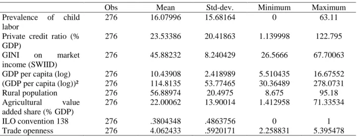
Table 1 : Descriptive Statistics
Obs Mean Std-dev. Minimum Maximum
Prevalence of child labor
276 16.07996 15.68164 0 63.11
Private credit ratio (% GDP)
276 23.53386 20.41863 1.139998 122.795
GINI on market income (SWIID)
276 45.88232 8.240429 26.5666 67.70063
GDP per capita (log) 276 10.43908 2.418989 5.510435 16.67552 (GDP per capita (log))² 276 114.8135 53.77465 30.36489 278.0731
Rural population 276 56.88974 20.4975 8.675 95.18 Agricultural value added share (% GDP) 276 22.00062 13.90014 1.412958 71.33534 ILO convention 138 276 .3804348 .4863756 0 1 Trade openness 276 4.062433 .5920171 2.258831 5.395478
Child labor is measured by the percentage of the population in the 10–14 year-old age bracket that is actively engaged in work. This include children, who, during the reference period performed “some work” for wage or salary, in cash or in kind at least 1 hour (Ashagrie, 1993). The structure of the data does not allow us to infer the intensity of child labor, so we cannot distinguish between light work (which some might argue is beneficial for adolescents) and fulltime labor, which might seriously conflict with human capital accumulation. Moreover, like most official statistics on child labor, these data are likely to suffer from underreporting, because work by children is illegal or restricted by law in most countries, and children often are employed in agriculture or the informal sector. These problems notwithstanding, the ILO data have the advantage of being carefully adjusted on the basis of internationally accepted definitions, thereby allowing cross-country comparisons over time (Ashagrie, 1993). To the extent that
5 Caution is required when exploiting the time aspect of the data. As in most countries, and especially in developing
economies, economic censuses are rare, the ILO relies heavily on projections (both intra- and extrapolations) for its estimates of economic activity rates. Thus, the reductions in child labor force participation rates will appear considerably smoother in the data than in the reality. In the paper, changes in child labor over ten-year periods are used that are relatively less affected by the issue.
17
underreporting is a time-invariant country characteristic or an overall time trend across countries, our fixed-effects estimator will not be subject to this bias. Data have been compiled by the International Labor Organization and are available on the World Development Indicators archives of the World Bank.
Nevertheless, it serves as the best available proxy for the prevalence of child labor in a cross-country panel setting and is widely used in empirical work (Ebeke 2012; Dehejia & Gatti 2005; Neumayer & de Soysa 2005; Kis-Katos 2007; Cigno et al. 2002).
Our preferred measure for inequality is the Gini coefficient of market income provided by the Standardized World Income Inequality Database created by (Solt 2014). He uses various techniques to estimate the ratios between different types of Gini coefficients relying heavily on information about the ratio for the same country in proximal times to increase the number of comparable observations. It combines data from the United Nations University’s World Income Inequality Database, the OECD Income Distribution Database, the Socio-Economic Database for Latin America and the Caribbean generated by CEDLAS and the World Bank, Eurostat, the World Bank’s PovcalNet, the UN Economic Commission for Latin America and the Caribbean, the World Top Incomes Database, the University of Texas Inequality Project, national statistical offices around the world, and academic studies. The data collected by the Luxembourg Income Study is employed as the standard.
As a measure for financial development, we use private credit by deposit money banks and other financial institutions to GDP. This indicator is a global measure assessing the size, depth and development of a country’s banking sector. It is limited as it does not capture the broad access to bank finance by individuals and firms, the quality and the efficiency of providing banking services. But, it is largely used as an indicator of financial development on macroeconomic studies and previous works on child labor, moreover recent data on financial access and the actual usage of banking services are not available before the 2000s. Series are drawn from the Financial Development and Structure Dataset, compiled by Beck, Demirgüc-Kunt and Levine, available on the World Bank website.
Data on child labor, the proportion of rural population, the share of agriculture value added in GDP, GDP per capita and the ratio of exports and imports to GDP are drawn from the
18
World Development Indicators of the World Bank, except for ratification of ILO convention 1386 establishing minimum working ages. The latter variable is a dummy taking the value 1 since a country has ratified the ILO convention and 0 otherwise. Basic summary statistics are presented in table 1 while partial correlations are available in appendix 1. In appendix 2 and 3, we present respectively by level of development and by region, evolution of child labor, inequality and financial development. Periods corresponds to the different decades between 1960 and 2000. We can notice that in all regions child labor is decreasing and it is the contrary for financial development. Regarding inequality, it is highly persistent in East Asia and Pacific, Latin America and Caribbean and in Middle East and North Africa regions; however it fluctuates more in South Asia and Sub-Saharan Africa (SSA). The highest figures are for SSA with an increase from 1960 to 1970 and a steadiness after. In South Asia, we can notice a decrease between 1960 and 1980, a rise of inequalities during the 90’s afterwards figures become stable.
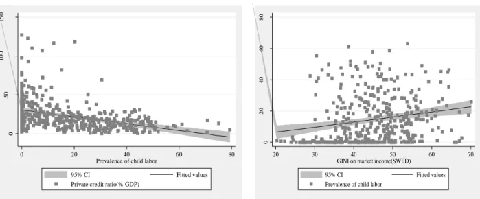
Figure 2 : Private credit and child labor Figure 3 : Inequality and child labor
Based on figure 1 and 2, we can notice that child labor is associated positively to inequality but negatively to financial development measured by private credit ratio to GDP. These graphs are simple correlations, so as to infer for causality, results of our empirical specification are presented in the next section.
6
Dates of ratification of the ILO Convention 138 can be found at the following address: http://www.ilo.org/dyn/normlex/en/f?p=NORMLEXPUB:11300:0::NO:11300:P11300_INSTRUMENT_ID:312283:NO. 0 50 1 0 0 1 5 0 0 20 40 60 80
Prevalence of child labor
95% CI Fitted values
Private credit ratio(% GDP)
0 20 40 60 80 20 30 40 50 60 70
GINI on market income(SWIID)
95% CI Fitted values Prevalence of child labor
19
4. Results
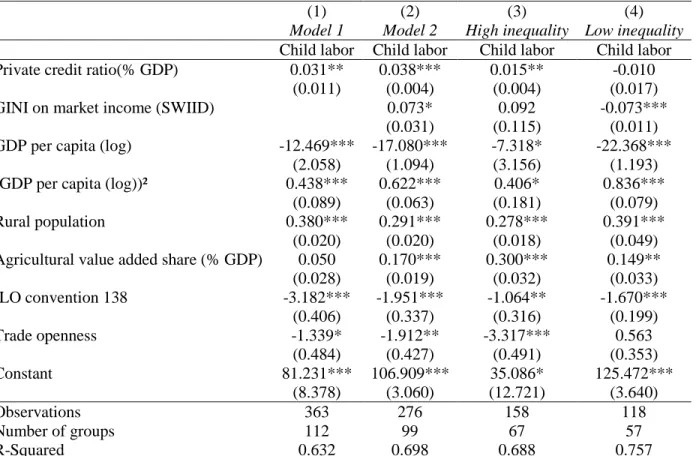
Table 2 : Results with fixed-effects
(1) (2) (3) (4)
Model 1 Model 2 High inequality Low inequality Child labor Child labor Child labor Child labor Private credit ratio(% GDP) 0.031** 0.038*** 0.015** -0.010
(0.011) (0.004) (0.004) (0.017)
GINI on market income (SWIID) 0.073* 0.092 -0.073***
(0.031) (0.115) (0.011) GDP per capita (log) -12.469*** -17.080*** -7.318* -22.368***
(2.058) (1.094) (3.156) (1.193)
(GDP per capita (log))² 0.438*** 0.622*** 0.406* 0.836***
(0.089) (0.063) (0.181) (0.079)
Rural population 0.380*** 0.291*** 0.278*** 0.391***
(0.020) (0.020) (0.018) (0.049) Agricultural value added share (% GDP) 0.050 0.170*** 0.300*** 0.149**
(0.028) (0.019) (0.032) (0.033) ILO convention 138 -3.182*** -1.951*** -1.064** -1.670*** (0.406) (0.337) (0.316) (0.199) Trade openness -1.339* -1.912** -3.317*** 0.563 (0.484) (0.427) (0.491) (0.353) Constant 81.231*** 106.909*** 35.086* 125.472*** (8.378) (3.060) (12.721) (3.640) Observations 363 276 158 118 Number of groups 112 99 67 57 R-Squared 0.632 0.698 0.688 0.757
Robust standard errors in brackets where *, **, and *** indicate statistical significance at the 10, 5 and 1 percent levels. In the last two columns, we split our sample according to the mean of the level of inequality measured by the Gini on market income, high inequality refers to countries with level of inequalities above the mean of the Gini index and low inequality for countries with value below the mean.
Table 2 above provides the results of the fixed effect model. Columns (1) and (2) report estimates respectively for model 1 and model 2. In all specifications, child labor is positively associated to financial development. Income level appears to be a great determinant of child labor and we find evidence of a U shape relationship like Acaroglu and Dagdemir (2010).
We investigate whether our result is linked to inequality by splitting the sample according to the mean of the Gini on market income as we do not find evidence of a conditional effect by introducing an interactive term between inequality and private credit7. In column (3), we report results for countries with high income inequality (above the mean of our sample) and in column (4), for countries with low inequality (below the mean). We find that it is only for high inequality countries that the effect is significant and positive even if we have a negative sign in countries where income inequalities are lower; it is not significant.
20
Table 3 : Results with instrumental variables
(1) (2) (3) (4)
Model 1 Model 2 High inequality Low inequality Child labor Child labor Child labor Child labor Private credit ratio(%
GDP) 0.339** 0.232* 0.268** -0.100** (0.075) (0.074) (0.078) (0.034) L.GINI on market income(SWIID) 0.096** (0.017)
(GDP per capita (log))² 0.576** 0.874*** 0.511 0.854***
(0.139) (0.069) (0.277) (0.109)
GDP per capita (log) -21.240*** -28.868*** -18.205* -21.763***
(4.183) (3.431) (7.879) (1.994)
Rural population 0.143*** 0.296*** 0.061* 0.341***
(0.016) (0.037) (0.025) (0.059)
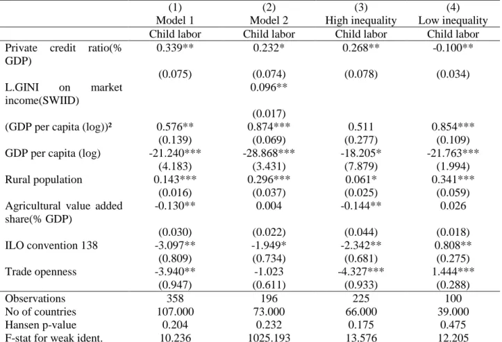
Agricultural value added share(% GDP) -0.130** 0.004 -0.144** 0.026 (0.030) (0.022) (0.044) (0.018) ILO convention 138 -3.097** -1.949* -2.342** 0.808** (0.809) (0.734) (0.681) (0.275) Trade openness -3.940** -1.023 -4.327*** 1.444*** (0.947) (0.611) (0.933) (0.288) Observations 358 196 225 100 No of countries 107.000 73.000 66.000 39.000 Hansen p-value 0.204 0.232 0.175 0.475
F-stat for weak ident. 10.236 1025.193 13.576 12.205
Robust standard errors in brackets where *, **, and *** indicate statistical significance at the 10, 5 and 1 percent levels. In the last two columns, we split our sample according to the mean of the level of inequality measured by the Gini on market income, high inequality refers to countries with level of inequalities above the mean of the Gini index and low inequality for countries with value below the mean of 44.
At this stage, due to the plausible endogeneity of financial development and inequality, our coefficients could be biased. So we report in table 3, results for the estimations with our instruments using the Limited Information Maximum Likelihood (LIML) estimator.
In order to be able to interpret our tests, we were obliged to partial out some variables like time fixed effects. By the Frisch-Waugh-Lovell (FWL) theorem in LIML, estimation of the coefficients for the remaining regressors are the same as those that would be obtained if the variables were not partialled out (Schaffer 2015). The relevance of the instruments is assessed through the Hansen test of overidentifying restrictions. Based on the Hansen p-values, we cannot reject the null hypothesis that the instruments are uncorrelated with the errors terms and that the excluded instruments are correctly excluded from the estimated equation. In addition, we report the Wald F statistic based on the Kleibergen-Paap (2006) rk statistic which is superior to the standard Cragg-Donald (1993) statistic in the presence of heteroskedasticity and autocorrelation.
21
The reported statistics are above the Stock and Yogo (2005) critical values and above the value of 10 as suggested by the “rule of thumb” of Staiger and Stock (1997). In order to deal with remaining endogeneity, we use the lag of the Gini coefficient following (Combes et al. 2014; Aggarwal et al. 2011).
We now turn to the discussion of results derived from the estimation factoring for endogeneity. We keep the same order for the columns as in table 2. Once again, the effect of financial development on child labor is positive. When we split the sample according to the mean of the Gini index like previously, we find that the impact still positive for countries with higher inequalities but for countries with lower levels, the coefficient is now negative and significant. In other words, financial development is efficient in reducing child labor for low level of inequalities otherwise we have the reverse effect with financial deepening leading to more child labor. We also notice that endogeneity tend to underestimate the effects of financial development on child labor given the magnitude of the coefficients comparing table 2 and table 3. Based on Table 3 and column (2), a one standard deviation increase in private credit (21.6) is associated to a 37 %8 increase in child labor relative to the mean of the sample (13.57).
In Table 4 below, we present the results when we introduce regional dummies and split our sample according to the level of income. In the first four columns, we add interactions between region dummies and the measure of financial development9. The reasoning is to test for a specific regional effect of private credit. We notice that the marginal effect of being a country of Sub-Saharan Africa and East Asia –Pacific is positive which is in line with our previous findings while for Latin America and the Caribbean, it is not significant. In fact, Sub-Saharan Africa and East Asia –Pacific are the countries with the highest prevalence of child labor. Surprisingly, the marginal impact of private credit conditional of being a country of Middle East and North Africa is negative. For explanation, we can refer to appendix 3, it is only in this region that inequality is decreasing during all the period and it also has the fastest growth of its financial system according to our measure of financial development. So in this region, financial development has evolved while inequalities have declined and this could explain the decreasing level of child labor. In other words, the impact of improving financial access for the poor is very effective in Middle East and North Africa compared to the other regions.
8
The following calculation has been made: (0.232 * 21.6/13.57) = 0.37.
22
Table 4: Regional and income specificities
(1) (2) (3) (4) (5) (6)
SSA LAC EAP MENA Low
income
Lower middle income Child labor Child labor Child labor Child labor Child labor Child labor Private credit ratio(% GDP) 0.336** 0.208** 0.055* 0.535*** 0.391** -0.086* (0.098) (0.072) (0.025) (0.090) (0.130) (0.039) (GDP per capita (log))² 0.538** 0.457** 0.317** 0.691* 0.463* -0.051 (0.117) (0.156) (0.112) (0.265) (0.212) (0.086) GDP per capita (log) -21.023*** -15.910** -10.548** -27.396** -21.082*** 1.589 (3.044) (4.755) (2.842) (6.787) (3.245) (2.742) Rural population 0.108** 0.165*** 0.164*** 0.140** 0.005 0.020 (0.025) (0.011) (0.019) (0.046) (0.028) (0.043) Agricultural value added share(% GDP) -0.144*** -0.100** -0.073** -0.177** -0.065*** 0.003 (0.027) (0.034) (0.016) (0.059) (0.014) (0.035) ILO convention 138 -3.727*** -2.820*** -1.381* -3.866** -3.952*** -0.173 (0.571) (0.575) (0.528) (0.935) (0.533) (0.324) Trade openness -4.143** -2.927** -2.337** -5.567** -2.856 -2.997** (1.411) (0.792) (0.692) (1.565) (1.583) (0.965) Private credit-ssa 0.323** (0.097) Private credit-lac 0.154 (0.121) Private credit-eap 0.045* (0.019) Private credit-mena -0.235** (0.077) Observations 358 358 358 358 160 127 No of countries 107.000 107.000 107.000 107.000 48.000 38.000 Hansen p-value 0.381 0.303 0.379 0.203 0.168 0.222
F-stat for weak ident.
31.059 32.491 24.117 2.709 33.135 11.028
Robust standard errors in brackets where *, **, and *** indicate statistical significance at the 10, 5 and 1 percent levels. In the last two columns, we split our sample according to the mean of the level of inequality measured by the Gini on market income, high inequality refers to countries with level of inequalities above the mean of the Gini index and low inequality for countries with value below the mean of 44.
23
4.1.
Robustness check
Table 5: GMM estimation and use of another credit variable
(1) (2) (3) (4) (5) (6) GMM GMM IV IV IV IV High inequality Low inequality
Model 1 Model 2 High inequality
Low inequality Child labor Child labor Child labor Child labor Child labor Child labor Private credit ratio(%
GDP) 0.0714** -0.1076* (0.0350) (0.0633) GINI on market income(SWIID) 0.2717** 0.0440 (0.1146) (0.1088) Domestic credit(% of GDP) 0.240*** 0.163** 0.175*** -0.053** (0.027) (0.047) (0.027) (0.019) L.GINI on market income(SWIID) 0.092* (0.029)
(GDP per capita (log))² 0.313** 0.780*** 0.323** 0.606*** (0.070) (0.067) (0.082) (0.093) GDP per capita (log) -14.4014** -14.4014** -12.697*** -24.677*** -10.477** -16.522***
(6.2914) (6.2914) (2.002) (2.612) (2.533) (2.146) Rural population 0.6020** 0.6020** 0.125*** 0.242*** 0.055 0.301*** (0.2748) (0.2748) (0.019) (0.023) (0.032) (0.055) Agricultural value added share(% GDP) -0.1154 -0.1154 -0.135*** 0.012 -0.080** -0.027 (0.1310) (0.1310) (0.016) (0.017) (0.022) (0.017) ILO convention 138 0.1427 0.1427 -2.737** -2.089** -2.048** -0.348 (0.1057) (0.1057) (0.642) (0.635) (0.592) (0.185) Trade openness -1.2237 -1.2237 -3.022*** -1.553* -2.508*** 0.370 (1.2969) (1.2969) (0.555) (0.491) (0.524) (0.288) Observations 158 118 442 214 298 116 No of countries 67 57 123.000 78.000 83.000 45.000 Hansen p-value 0.495 0.358 0.202 0.2359 0.4811 0.278 AR2 0.151 0.607 Number of instruments 38.000 29.000
F-stat for weak ident. 393.214 493.074 386.702 54.332
Robust standard errors in brackets where *, **, and *** indicate statistical significance at the 10, 5 and 1 percent levels, respectively. Endogenous variables are Private credit ratio and Gini on market income (inequality) for GMM estimation.
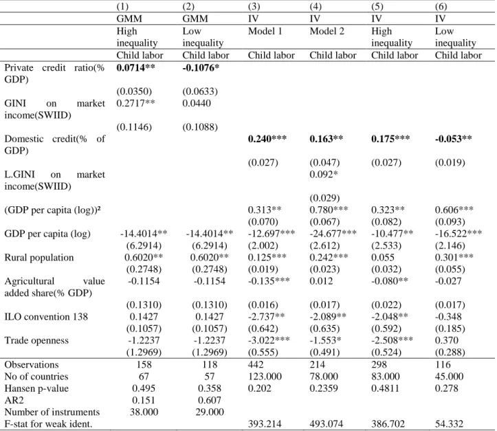
In table 5 above, we test the robustness of our results by using a GMM estimation which is more robust in case of measurement errors, over-identified models, non-spherical error terms and weak instruments. As previously, we split our sample according to the mean of the Gini coefficient. Columns (1) and (2) report results respectively for the countries above and below the mean. Once more, we find that the positive effect of financial development on child labor is driven only by countries with high income inequality. In Countries where the Gini index is below
24
the mean for the sample, the effect is negative and significant. In the last four columns, we use an alternative measure of financial development namely domestic credit to the private sector which is also a measure of financial deepening. The difference is that this indicator includes credit to public enterprises. Once again, our results are quite similar to those obtained with private credit to GDP.
In order to verify that our results are not sensitive to the use of averages over ten years, we also run our regressions using the averages over five years. Once again our previous results are confirmed, child labor is related positively to financial development and this result is driven by countries with high inequalities (see Appendix 7 for more details).
4.2.
Introducing institutional quality
We also look at if our results are not conditional to institutional quality. Based on our literature review, the positive effect of financial development on child labor could be linked to the high opportunity cost of education. In this line, we want to test the idea that in countries with good institutions and governance, there is a better quality of education reducing the impact of the high opportunity cost of education in parents’ choice of child labor in the case they use credit to invest in family firm or business. In fact, parents’ decision whether to send a child to work or/and to school depends essentially on three things: the cost (including the opportunity-cost) of education, the expected return to education, and the extent to which parents are able to finance educational investments (Cigno et al. 2002). Especially, households would rationally prefer child labor if the high opportunity cost of education is associated to a lower marginal benefit from schooling. Consequently, we argue that policies which tend to improve the quality of education raising its return can reduce child labor, this could be done through better bureaucracy quality and fewer corruption for example. In order to test this conditional effect, we introduce an interactive term between private credit ratio and institutional variables taken from International Country Risk Guide (ICRG) which are more pertinent for the provision of public services namely corruption, bureaucracy quality, democratic accountability, and law and order10. For endogenous interactive terms, we multiply the instruments for private credit ratio (existence of public credit
25
registry and private credit bureau) by the exogenous institutions variables (Bun et al. 2014; Wooldridge 2002).
Table 6 : Controlling for institutional quality
(1) (2) (3) (4) (5) (6) Child labor Child labor Child labor Child labor Child labor Child labor Private credit ratio(% GDP) 0.171*** 0.176*** 0.194** 0.454*** 0.177*** 0.173*
(0.027) (0.034) (0.070) (0.141) (0.019) (0.090) L.GINI on market
income(SWIID)
0.048*** 0.045** 0.046** 0.045 0.048*** 0.014 (0.014) (0.019) (0.017) (0.026) (0.011) (0.020) (GDP per capita (log))² 0.589*** 0.487*** 0.524*** 0.570*** 0.634*** -0.210* (0.080) (0.120) (0.129) (0.144) (0.072) (0.101) GDP per capita (log) -16.954*** -15.980*** -16.756*** -22.844*** -17.732*** 5.745* (2.449) (3.751) (4.541) (6.530) (2.588) (3.055) Rural population 0.126*** 0.168*** 0.126*** 0.118** 0.129*** 0.227***
(0.019) (0.022) (0.019) (0.046) (0.015) (0.026) Agricultural value added
share(% GDP) -0.010* -0.032 0.001 -0.022 -0.010 -0.002 (0.005) (0.019) (0.012) (0.037) (0.008) (0.003) ILO convention 138 -0.806*** -1.025*** -1.114*** -1.606** -0.760*** -0.336** (0.163) (0.187) (0.300) (0.600) (0.146) (0.134) Trade openness -0.534* -0.437 -0.506 -0.939 -0.643*** -0.158 (0.258) (0.337) (0.408) (0.670) (0.164) (0.317) Corruption 0.411 0.686** (0.281) (0.320) Private credit ratio*Corruption -0.024*** -0.034*** (0.007) (0.010)
Law and Order -0.716** (0.296) Private credit ratio*Law and
Order 0.005 (0.010) Democratic Accountability 0.101 (0.202) Private credit ratio*Democratic Accountability -0.005 (0.006) Bureaucracy Quality 0.218 0.156 (0.595) (0.264) Private credit ratio*Bureaucracy Quality -0.035** -0.000 (0.013) (0.005) Corruption(Heritage) 0.125* (0.058) Private credit ratio*Corruption(Heritage) -0.004** (0.002) Observations 1129 1129 1129 1129 1129 860 No of countries 82.000 82.000 82.000 82.000 82.000 99.000 Hansen p-value 0.446 0.485 0.439 0.474 0.631 0.4123 F-stat for weak ident. 11.265 29.940 11.864 11.817 8.029 8.789 Robust standard errors in parentheses, * p < 0.1, ** p < 0.05, *** p < 0.01
26
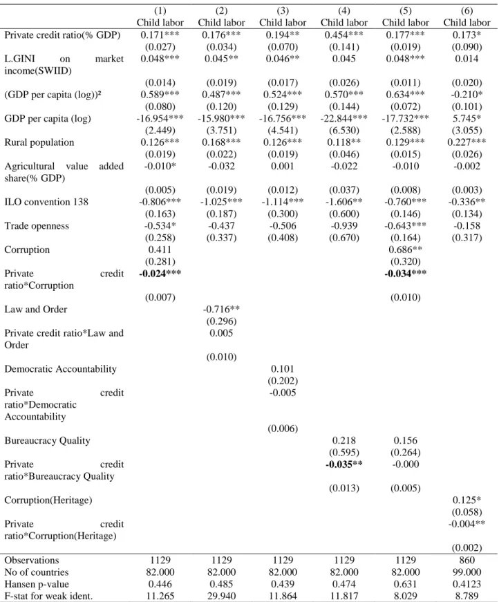
Results are presented in Table 611, we introduce separately the interactive term with each variable of institutional quality from column (1) to column (4), then in column (5) we introduce simultaneously the interactive terms which were significant separately. We find that private credit ratio is effective in reducing child labor only in countries with better control of corruption and bureaucratic quality. When we introduce jointly the interactive terms for this two measures of institutions, it is only the interaction with corruption which remains significant. This was predictable, given the high correlation between these variables and the fact that corruption affects directly bureaucratic quality. We also use an alternative measure of corruption from the Heritage foundation which has rescaled the Corruption Perception Index (CPI) of Transparency International12. The result presented in column (6) is similar with the negative impact of private credit observed for initial low level of corruption. These findings are rationale as corruption has been demonstrated to have a negative impact on social and political development of countries undermining the efficiency of public services. We can take for example the seminal case of Kenya, where a Public Expenditure Tracking Survey (PETS) emphasized that in the period 1991-1995, schools received only 13 percent of funds dedicated to cover non-wage expenditures. The bulk of the school grant was captured by local officials (and politicians), within the scope of leakages (Reinikka & Svensson 2004). Moreover, schools in better-off communities managed to receive larger share of funds, enhancing inequalities. In Kenya, it is only 20 percent of schools which received their funds (Glassman et al. 2008). But Since 2003, cash is directly transferred from the central government to the school’s bank account, which helps eliminating leakage further underlying the importance of financial development.
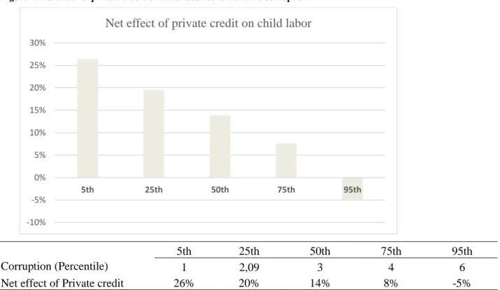
In Figure 4 below, we calculate the net effect of financial development on child labor for different percentile levels from column (5) in Table 6. We can observe that this effect become negative only after the 75th percentile for corruption which corresponds to the best level of good governance13. We derive that a one standard deviation increase in private credit ratio to GDP (24.12) is associated with a 5%14 decrease in child labor relative to the mean (13.10) for a
11
We do not use five or ten years average as to taken into account all the available data and the variability of institutional quality.
12 The Index converts the raw CPI data to a scale of 0 to 100 by multiplying the CPI score by 10. For example, if a
country’s raw CPI data score is 5.5, its overall freedom from corruption score is 55.
13
The indicator of corruption varies between 1(high level of corruption) to 6 (minimum degree of corruption).
27
developing country with a corruption index that corresponds to 95th percentile of the distribution of the variable (6).
Figure 4: Net effect of private credit on child labor conditional to corruption
5th 25th 50th 75th 95th
Corruption (Percentile) 1 2,09 3 4 6
Net effect of Private credit 26% 20% 14% 8% -5%
4.3.
Controlling for the provision and the efficiency of education
services
In this section, we want to test directly if the provision of education services and their efficiency could help reduce directly child labor in developing countries. Following (Neumayer & de Soysa 2005); we add as additional controls, the ratio of public expenditures in education to GDP which is more relevant to assess if the provision of education services is a priority for the government. But it doesn’t give information about the quality or the efficiency of the education system which can really impact the return from education. So we introduce the survival rate to grade five or the share of primary schools entrants that reach this grade, we choose this indicator as it has more observations than other measures like the pupil to teacher ratio for our period of analysis (1960-2004). All these data are drawn from the World development Indicators of the World Bank. Ideally, we would also like to have indicators which directly measure the marginal benefit from
-10% -5% 0% 5% 10% 15% 20% 25% 30% 5th 25th 50th 75th 95th
28
education like the graduate unemployment rate. We do have data on unemployment with secondary or primary education, unfortunately they are not suited for international comparisons as age group, geographic coverage, and collection methods could differ by country or change over time within a country. Besides these limitations to comparability raised for measuring unemployment, the different ways of classifying the education level may also cause inconsistency across countries. Still, information on educational attainment is the best available indicator of skill levels of the labor force to date (WDI, 2016)15.
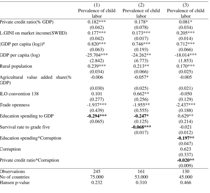
Table 7: additional controls for education services and efficiency
(1) (2) (3) Prevalence of child labor Prevalence of child labor Prevalence of child labor
Private credit ratio(% GDP) 0.182*** 0.178* 0.081*
(0.042) (0.078) (0.034)
L.GINI on market income(SWIID) 0.177*** 0.173*** 0.205***
(0.042) (0.017) (0.014)
(GDP per capita (log))² 0.820*** 0.746*** 0.712***
(0.063) (0.193) (0.066)
GDP per capita (log) -25.704*** -24.262** -18.014***
(2.842) (6.773) (1.853)
Rural population 0.239*** 0.213** 0.170***
(0.034) (0.066) (0.025)
Agricultural value added share(% GDP) -0.006 -0.057* -0.005 (0.030) (0.025) (0.021) ILO convention 138 0.101 0.662** -0.050 (0.277) (0.256) (0.129) Trade openness -1.937*** -1.955** -2.437*** (0.439) (0.555) (0.188) Education spending to GDP -0.294*** -0.247* 0.629** (0.065) (0.125) (0.214)
Survival rate to grade five -0.068*** -0.021
(0.017) (0.012)
Education spending*Corruption -0.197**
(0.047)
Corruption 0.623
(0.337)
Private credit ratio*Corruption -0.020**
(0.009) Observations 245 161 130 No of countries 75.000 53.000 45.000 Hansen p-value 0.232 0.310 0.466 15
This is based on the suggestions of the Word Development Indicators (2016) of the World Bank for the use of unemployment data.
29
F-stat for weak ident. 23.496 10.082 2.026
Anderson-Rubin F-stat 36.062 66.704 43.705
Robust standard errors in parentheses, * p < 0.1, ** p < 0.05, *** p < 0.01.
Our results are presented in Table 7 above. In column (1) and (2) we introduce respectively the level of education spending and the survival rate to grade five in primary education. We observe that the coefficient for public expenditure is negative and significant at 1% level in the first column. As soon as, we introduce the share of primary school entrants that reach grade five, the coefficient of education spending is reduced and less significant (10%), it is now the survival rate which has a negative effect on child labor. This may be due to the fact that the survival rate better captures the provision of education services and acts as a transmission channel for the impact of education expenditures.
In column (3), we test whether public education spending is more effective in reducing child labor in case of a better control of corruption like for the ratio of private credit. For instance, Mauro (1998) highlights that Corruption is likely to reduce government spending on education at the expense of other sectors like fuel and energy. This is similar to the findings of Delavallade (2006) for a panel of developing countries. An explanation is that corrupt governments find it easier to collect bribes in these sectors. Moreover, Rajkumar and Swaroop (2008) demonstrate that public spending in education is more effective in increasing education attainment in countries with good governance, in other words, with less corruption. So, we introduce an interactive term between education spending and corruption, we also add an interaction between private credit and corruption in column (3). Once again with all these interactive terms, financial development helps reduce child labor in presence of better control of corruption, this is also the case for education spending. This finding is closed to the previous results cited concerning the efficiency of public expenditures, the difference is that rather than focusing on education attainment, our variable of interest is child labor.