Argon diffusion gradients in micas and implications for the thermal history of the Sandia pluton

Argon Diffusion Gradients in Micas and Implications

for the Thermal History of the Sandia Pluton

by

Ellen A. Dotson

B.S., Earth, Atmospheric and Planetary Sciences

Massachusetts Institute of Technology, 1993

Submitted to the Department of Earth, Atmospheric, and Planetary

Sciences in Partial Fulfillment of the Requirements for the Degree of

Master of Science

at the

Massachusetts Institute of Technology

August 1994

Copyright ©1994 Massachusetts Institute of Technology

Signature of Author

Certified by

- _ --- -_ -_

--Department of Earth, Atmospheric, and Planetary Sciences August, 1994

(

Thesis Supervisor

Accepted

by-.-/

SEP -BRAM

Thomas H. Jordan

Department Head

~~---I---Argon Diffusion Gradients in Micas and Implications

for the

Thermal History of the Sandia Pluton

Ellen A. Dotson

Submitted to the Department of Earth, Atmospheric, and Planetary Sciences on August 23, 1994 in partial fulfillment of the requirements for the

Degree of Master of Science in

Earth, Atmospheric, and Planetary Sciences

Abstract

Micas from slowly cooled terranes can contain significant age gradients produced by thermally-activated diffusion of argon. Previously published work (Dodson, 1986) has shown that the distribution of apparent ages in such samples can yield important thermal history information, but the method used was predicated on the assumption that T-1 increased' linearly with time. Using a finite difference approximation of the diffusion equation to simulate argon gradients for an assortment of slow-cooling T-t paths, I show that Dodson's (1986) equation predicts closure temperature profiles and integrated cooling rates over the closure interval with reasonable accuracy regardless of the functional form of the T-t curve. Because closure intervals can vary greatly as a function of composition and size, a collection of diverse micas with age

gradients from a slowly cooled terrane can define a cooling path with great detail. The usefulness of this approach is illustrated with a suite of micas from the Sandia pluton, a - 1.45 Ga anorogenic granite in central New Mexico. 4 0_Ar/3 9_{Ar laser microprobe analyses indicated apparent age gradients that} exhibit ranges up to 450 Ma in age in an individual crystal. The integrated cooling rates obtained from these micas, define a cooling history which suggests a transient thermal pulse related to emplacement of the pluton,

followed by a remarkably stable, protracted (> 500 Ma) slow cooling (<< 1 K/Ma).

Acknowledgments

I would like to thank Kip Hodges for his insight, guidance, humor, and considerable patience as an editor, without which this thesis would never have

seen the light of day.

My friend Nicholas Roosevelt has my deep gratitude for his steadfast faith and patience throughout this year. He is the best of companions.

My deepest gratitude goes to my parents, Margaret and Adrian Dotson, whose steady love and support has been, and always will be, the most valuable of gifts.

Table of Contents

2. Modelling Volume Diffusion of Argon in Biotite 16

2.1 Introduction 16

2.2 Equations of Diffusion 17

2.3 Requirements of a Geologically Useful Solution to the Diffusion Equation 19 2.4 Forward Modelling with Finite Difference Methods 21

2.5 Results and Discussion 23

3. Thermal History of the Sandia Pluton 27

3.1 Introduction 27

3.2 Regional Geology 28

3.3 Statement of Purpose 31

3.4 Experimental Techniques 31

3.5 Individul Results 34

3.6 Discussion and Suggestions for Further Study 36

4.Conclusions 42 References 43 Table Captions 45 Tables 46 Figure Captions 57 Figures 59

Chapter 1

Introduction

In order to understand cooling histories of geologic materials,

geochronologists rely on several assumptions regarding the diffusion of

radiogenic daughter isotopes out of mineral systems. Thermally-activated

diffusion is thought to be a primary mechanism for the loss of daughter

isotopes. To relate apparent age to the cooling history of a sample,

geochronologists rely on a mathematical equations (Dodson, 1973; Dodson,

1986) derived from a solution to the diffusion equation. The validity of these equations depends on a number of assumptions being correct: the mineral is

assumed to be initially in equilibrium with its environment; the diffusion

parameters for various mineral systems must be known; and this solution is

exactly true only when T-1 increases linearly with time. In order to test the

reliability of Dodson's equations for samples which experience cooling

histories that are not linear with T-1, a numerical finite difference

approximation of the diffusion equation was utilized to model argon gradients

for a variety of cooling histories. These results were then compared to the

predictions made by Dodson's solution.

1.1

Diffusion

Diffusion is the mechanism by which molecules are transported

through some medium by the random molecular motions. Imagine a system

with a finite amount of diffusing component X, which initially has a

high-concentration region (region A) with a high-concentration of XA, and a

diffusing component in the system, each motion step is entirely random. An

individual X has an equal probability of moving either towards or away from

region A during any single step. At any one instant, a constant percentage of

the total number of X is moving away from A and toward B. An equal

percentage is moving towards A and away from B. Now imagine a plane which

separates A and B. A constant percentage of XA, crosses the boundary into

region B, while an equal percentage of XB, crosses the boundary into region A.

But, because there is a higher absolute number of X in region A, there will be a

net transport of X from A into B until, over time, both sides have the same

concentration of X. The system is then said to be in equilibrium with respect to

X (cg. Crank, 1975; Shewmon,1989)

In geochronological systems, the diffusing component of interest is the

daughter product of some radioactive parent isotope with a known half-life.

Initially upon crystallization, a mineral will be at isotopic equilibrium with its

surrounding environment with respect to the daughter product. The ambient

concentration of the daughter product is incorporated into the crystal

structure. In the case of thermally-activated diffusion, as the mineral cools

and the daughter product is being produced by radioactive decay, the daughter

product will take random steps with a lower frequency and the crystal lattice

will become more "rigid". This process makes it more difficult for the daughter

product to move from place to place within the crystal. If the concentration of

the daughter product is higher within the mineral than in its surrounding

environment, equilibrium requires the daughter product to diffuse out of the

mineral. As a mineral cools, the daughter product diffuses less rapidly out of

the mineral system. When the production rate is greater than the loss due to

diffusion, the mineral system retains some portion of the daughter product,

diffusivity of a system can be qualitatively thought of as a measure of the ease

with which a particular diffusing component can move through a particular

medium, given a certain set of conditions, such as temperature, pressure,

chemical composition of the mineral and quantity of vacancies within the

medium.

1.2

_Ar/

_Ar

_{Thermochronology}

Traditional 4 0Ar/3 9Ar thermochronologic studies utilize the varying

thermal diffusivities of argon in different minerals to constrain the

temperature-time history of a sample. The fundamental assumption of this

approach is that the primary argon-loss mechanism is thermally activated

diffusion of the sort described above. For thermally activated diffusion, D, the

diffusivity, follows an Arrhenius relationship,

D =D _oexp[- ] (1)

where E is the activation energy, R is the universal gas constant, T is

temperature and Do is the diffusivity at infinite temperature. It can be

observed from this relationship that D is strongly dependent upon the

temperature of the system. Above some critical temperature range the

mineral loses virtually all of the radiogenic argon as. it is being produced;

below this critical temperature range, essentially, all of the radiogenic argon

produced in a mineral is retained. The rate at which a sample cools through

this transitional temperature range has a profound effect upon argon

retention, and subsequently, on the extent of time-temperature information

For example, if a specimen undergoes rapid cooling, as it would in a

volcanic or hypabyssal setting, the sample rapidly traverses the transitional

temperature ranges of the K-rich minerals. The apparent

Ar/

Ar ages of

assorted K-rich minerals from a single sample will be virtually identical to one

another and to the crystallization age of the mineral.

In contrast, when a sample undergoes moderate cooling, different

K-rich minerals from the same specimen will exhibit significantly disparate

apparent

Ar/

Ar ages due to the differing diffusivities of argon in

different mineral systems.

Dodson (1973), presented an equation derived from a solution to the

diffusion equation;

Tc =R/[E In(A

T

which gives the integrated closure temperature as a function of E, Do, A (a

constant depending on diffusion geometry of the mineral and the radioactive

decay rate), a (the characteristic diffusion radius of a particular mineral), and

T (the time constant). T, the time constant is defined as,

= - R T2/(E dT/dt)

(3)

Equation (2) is exactly true only when T-1 increases linearly with time. The

integrated apparent

Ar/

_{Ar age records the time at which a particular}

mineral passes through the closure temperature predicted by this equation. By

applying this method to a variety of K-rich minerals from a geographic

region, one can constrain the temperature-time history of a tectonic region.

When a mineral experiences slow cooling through its transitional

temperature range, a measurable concentration gradient of the diffusing

component will be developed within the mineral grain. This occurs because as

the sample cools, the mean distance the diffusing substance will travel during

a unit time decreases (Shewmon, 1989). A daughter product originating in the

center of the grain must travel a greater distance to reach the free surface at

the grain boundary, and thus has a smaller probability of escaping the system.

The mean distance traveled in a unit time decreases as the system cools, while

the production rate remains constant. The center of the mineral begins to

retain radiogenic argon, while daughter product in the outer portion of the

grain remains in equilibrium with the environment. Over time, a concentric

gradient, with higher concentrations in the center and lower concentrations

near the edge, will be developed as the system passes through the transitional

temperature range. This gradient should be measurable when the time taken

to traverse the critical temperature range is longer than the experimental

uncertainty associated with the 4 0Ar/3 9Ar dating technique.

Dodson (1986) presented the following equation which predicts the

spatial distribution of closure temperatures for samples which have

undergone slow cooling.

E/RTc = G(x)+

1T

D

/a2)

(4)

G(x) is a geometric term which depends upon the diffusion geometry of the

mineral and the position x within the mineral, and a is the grain radius. Once

again, this equation is exactly true only when T- lincreases linearly with time.

This equation provides a way to constrain a portion of the temperature-time

path by analyzing the radiogenic argon gradients within a single mineral

In recent work by Hames and Hodges (1993) and Hodges et al. (1994),

significant age gradients were measured in individual muscovite and biotite

and biotite grains. In the study by Hodges et al. (1994), individual muscovite

and biotite grains from the Crazy Basin monzogranite from central Arizona

were analyzed. Spot fusion mapping of the {001} cleavage plane using a

focused 10W-Ar laser revealed broadly concentric age gradients from 1650 ma

to 1270 Ma in the muscovite sample, and from 1420 Ma to 1150 Ma in the biotite

sample. Assuming that these gradients were developed by thermally activated

diffusion, they utilized equation (4), to obtain an integrated cooling rate of

-0.30 K/m.y. through the transitional temperature range for the muscovite,

and a cooling rate of -0.33 K/m.y. for the biotite. They argued that the

agreement between these results provides persuasive evidence for very slow

cooling of the Crazy Basin monzogranite.

There is no geological reason to justify an a priori assumption that all

regions which undergo slow cooling follow a cooling path in which T- 1

increases linearly with time. The question arises, what would be the

morphology of diffusion gradients in minerals which undergo slow cooling

along other cooling paths? Do these gradients differ significantly from

gradients formed by linear T-1 cooling? Given these gradients, if one applies

Dodson's 1986 method, how well does his integrated cooling rate approximate

the different cooling rates through the transitional temperature range? The

second chapter of this thesis attempts to answer these questions, by forward

modeling diffusion gradients for a variety of cooling curves that are not

linear with T-1 using finite difference techniques, and the then comparing

As will be shown in chapter 2, equation (4) does a good job of predicting

the closure temperatures and cooling rates based on gradients developed by

slow cooling paths not necessarily linear with T-1. It is possible to define a

portion of a cooling curve that is not linear with T-1, by using equation (4),

with gradients developed in a number of minerals of different sizes and

compositions. The size and composition of a mineral has a profound effect on

the transitional temperature range, and thus records different portions of the

cooling history. The third chapter presents argon microprobe data from a

suite of micas from the Sandia pluton in New Mexico. The cooling rates

predicted by equation (4) for these micas collectively form a coherent cooling

curve that is not linear with T-1. These results suggest that it is possible to

define detailed cooling histories in slowly cooled terranes by analysis of argon

Chapter 2

Modeling Volume Diffusion of Argon in Biotite

2.1

Introduction

A number of recent studies (Hames and Hodges, 1993; Hodges et al, 1994)

have mapped out argon gradients on individual mica grains. These gradients

were interpreted to be diffusion gradients formed by thermally-activated

diffusion. The gradients were broadly concentric, with older ages at the

center, and younger ages at the rim. This age profile, if developed by

thermally activated diffusion, indicates that the effective diffusion radius of

mica is the size of the grain. The age gradients were used to calculate cooling

rates by applying Dodson's (1986) equation relating closure temperature and

cooling rate to age and position.

Dodson's (1986) equation is exactly true only when T- 1 _increases

linearly with time, and therefore we must ask ourselves how well does

equation (4) predict cooling rates when T-1 is not linear with time. This study

focuses on the application of finite difference analytical methods to predict

the morphology of argon gradients in biotite developed by thermally activated

diffusion. This approach easily allows one to predict argon gradients for a

variety of cooling rates and initial argon gradients. The morphology of argon

gradients in biotite is forward modeled for a variety of temperature-time

paths. The predicted concentration gradients are then converted to age

gradients and closure temperature profiles. The modeled gradients are

compared with Dodson's predicted gradients to gain insight into the robustness

2.2

The Diffusion

Equations

In 1855 Aldof Fick set forth the fundamental equations describing the

process of diffusion. He recognized that the process of material diffusing

through a medium was parallel to the diffusion of thermal energy through a

system, and adapted Fourier's Law of Heat Conduction to the diffusion of

material. Fick's first law states the flux of material through an area is

proportional to the concentration gradient. Specifically,

dc

J

= -D

,

(5)

dx

where J is the rate of transfer of material through a unit area, C is the

concentration of the diffusion material and D is the diffusion coefficient for

the system. The negative sign indicates that flux occurs in the direction

opposite that of increasing concentration. It is important to note that D is

independent of the concentration gradient (Shewmon, 1989).

The derivation of Fick's second law follows easily from Fick's first law

(Crank,1975). Suppose we have a rectangular parallelepiped whose center is at

point (x,y,z) and the length of the edges are 2dx, 2dy, and 2dz.

2dz

I

f

I A

B

2 d y

---2dx

Suppose we have some substance diffusing either into or out of our system. The

the change in concentration (i.e. amount per unit volume) per unit time,

multiplied by the volume of the object of interest, explicitly,

dC

8dxdydz

,

(6)

dt

where t is time. The rate at which the diffusing substance enters or leaves the

system can also be expressed as the sum of flux through each surface

bounding the system. For plane A, which is normal to the x axis passing

through point x - dx, the rate of material entering the system through this

plane is equal to

4dydz J

-

dx ,

(7)

where Jx is the flux through a plane normal through the x axis passing

through center point (x,y,z). Similarly the rate of material leaving the system

through plane B, which is normal to the x axis passing through point x + dx, is

equal to

4dydz Jx +

dx .

(8)

Thus, the rate of increase of the diffusing substance in the system due to flux

across these two planes is

- 8dxdydz x. (9)

dx

Similarly, the rate of increase due to flux across boundaries normal to the y

axis and z axis is equal to

-8dxdydz and-8dxdydz-z respectively. (10)

If we assume that the production of the diffusing substance within the system

is equal to zero then,

dC

J dJ

J

-=+ X 1 +

= 0.

dt

dx

dy

dz

If diffusion is isotropic, i.e. occurs equally in all directions, and is constant, then,

dC

(dCd

_{C d}

-

D

This equation is known as Fick's second Law. The diffusion of argon in biotite

is commonly thought to be cylindrical in geometry (Giletti, 1974; Harrison et

al, 1985). This equation can be transformed into cylindrical coordinates by

substituting,

x = rcos 0 and y = rsin 0.

Giving,

aC ₌ 1 8 ( r D c \ _rD- , ₊ D _{-- d} C - -c)}

+ rD- , (13)

t

r or

dr

A

r

A0

dz

dzJ

with cylindrical coordinates r,

0,

2.3 Requirements of Geologically

Useful

Solutions

to the

Diffusion

Equation

A geologically useful solution to the diffusion equation will include a

radiogenic production term for the diffusing substance of interest, and will

also take into account the time variance of D, the diffusivity coefficient.

Dodson's 1973 solution to the diffusion equation fulfills these requirements,

The loss of argon in biotite is thought to be due to thermally activated

diffusion. When the temperature of the system changes with time, D varies

with time. In order to solve the diffusion equation in this situation, a new time

scale is introduced.

D is taken to be some f(t); the new time scale, t, is defined such that,

dr = f(t) dt.

(14)

Fick's second law becomes,

dC

d

_C

_d

_C

_d

+ +

(15)

S dx2 dy2 Z2

Mathematical solutions for such diffusion equations are exactly true only for

the temperature-time path defined by f(t).

In Dodson's (1973) paper, he presented a solution which defined the

time scale t (equation 3), as the time constant for which D decreases by a

factor of e-1, when T- 1 increases linearly with time. The solution for mean

closure temperature (equation 2), requires the assumption that the mineral

starts out with the diffusing substance in equilibrium with the environment;

specifically, the diffusion of the daughter product is extremely rapid compared

to the production rate. This assumption makes equation (2) inappropriate in

situations where a mineral may experience partial loss of some daughter

product due to reheating. Dodson (1986) modified his solution to predict the

spatial distribution of closure temperatures (Tc) for a sample which has

undergone slow cooling (equation 4). Once again, this solution is

inappropriate for predicting gradients developed when there is partial loss

due to reheating and the equation is exactly true only when T-1 increases

2.4 Forward Modeling

with Finite Difference

Methods

histories, it is either necessary to find mathematical solutions for a variety of dT =

f(t)

approximation of the diffusion equation. The latter approach has the

advantage of flexibility, in that only one finite difference approximation can

be used for a variety of thermal histories.

If we assume that diffusion is radially symmetric and that diffusion

parallel to the c-axis negligible then the terms involving

dO

zero, leaving,

dC

1

[

(D

- -- -= rD ). (16)

If we introduce the following non-dimensional parameters,

R = r/a and T = Dt/a

,

(17)

where r is the distance from the center from the grain, and a is the radius of

the grain, equation (10) becomes,

C 1

(

dC

R = + - - (18)

dr

RdR

dR

dR

RdR

The finite-difference approximation for equation (18) is,

C

d

dC'

{(2i

1)Ci,j -4iC,

+(2i -1)C

-T R d RA 2i(3R)

where Ci,j is the concentration of the diffusing component of interest at point

(i8R, j&6), when the radius a has been divided into equal intervals of length SR,

For this study, equation (19) was modified to include a radiogenic

production term Aj, to form,

Cj

2

-

+(2i

1)Ci-i,

.

Aj is the amount of daughter product produced during the j-th time step,

normalized by the initial amount of the parent isotope, No. Aj was calculated

using,

A

(

j

where A, for potassium, is 5.543 x 10-10 a- 1_{. D, the diffusivity coefficient, was}

calculated for each time step assuming D followed an Arrhenius relationship

(equation 1), with Do = .077 cm2-sec- 1, E=47.0 kcal-mol-1 , as reported in

Harrison et al, 1985. The temperature is calculated as some function of time. For

all models presented in this study the edge of the grain was taken to be a free

surface with zero concentration of argon. This could easily be modified by

setting the concentration at a+6R equal to some amount other than zero during

each time step.

The finite difference modeling approach permits consideration of

specific variables in ways not possible with analytical solutions. The initial

concentration matrix, Cinitial, can be set equal to any desired concentration

gradient. This allows gradients to be predicted for minerals initially not in

equilibrium with their environment. This method also allows one to use a

variety of T=f(t) paths, allowing modeling of the effect of heating as well as

argon gradients developed in minerals which experience reheating due to a

short lived thermal pulse.

The finite difference numerical approximation for the diffusion of

argon in biotite (equation 20) was used for a variety of T-t paths shown in

Figures 1 and 2 (parameters in Table 1).

For all models presented in this study, the Cinitial was set equal to zero

in order to approximate the assumption in Dodson's (1986) mathematical

treatment that the grain is initially in equilibrium with the environment with

respect to argon. The initial temperature, for all models, was chosen to be 800 K

so that the diffusion of argon is initially very rapid relative to the production

rate for a grain with a diffusion radius of 1 cm.

2.5 Results and Discussion

To compare the numerical method to Dodson's (1986) treatment, the

parameters for Model A were chosen to agree with his assumptions of initial

equilibrium and linear cooling with T-1. The modeled concentration gradient

was converted to an age gradient using,

1 (D

t=- In 1 --. (22)

A closure temperature profile was then calculated by converting age to

absolute temperature based on the known cooling history used in Model A.

Figure 3 compares the modeled closure temperature profile for Model A, with

the closure profile predicted by Dodson's equation, using the same parameters.

closure profile is shown with a solid line. The agreement between closure

temperatures for these two methods are within 1% of the absolute temperature.

It useful to compare the forward modeled argon gradients for T-t Models

A-E. Due to the nature of the cooling trajectories, the traverse through the

transitional temperature range from 730K to 550K, occurred at significantly

different times. If we assume the argon accumulates more or less uniformly

throughout the grain after "closure", it seems reasonable to subtract the

amount of "additional" radiogenic argon trapped by the system after "closure",

in order to compare the morphology of the argon gradients at the time of

closure. These gradients were then normalized to facilitate comparison (Figure

4). The qualitative effect of cooling rate upon argon gradient morphology

becomes apparent. Model D which experienced the most rapid descent through

the transitional temperature range, has a plateau of relatively constant

concentration toward the center of the grain, with a definite shoulder at the

transition to lower concentrations towards the rim. This shoulder is

successively less pronounced with each model traversing the transitional

temperature range during a longer time span. Model E experiences the slowest

traverse, and its predicted argon gradient is smooth and round. The argon

gradient morphology approaches a straight line with a slope of -1, as the

cooling rate approaches zero. It may be possible to use this systematic

variation to estimate cooling rates for actual samples that exhibit broadly

concentric age gradients. Argon gradients observed in micas by spot fusion

analysis, could be normalized in the manner above, and then compared to a

plot of modeled gradients to provide a rough estimate of the cooling rate. This

method requires the assumption that the grain is in equilibrium with it's

this approach is that it provides a second way of estimating cooling rate,

entirely independent of Dodson's equation.

To gain insight into the ability of Dodson's method to predict closure

temperatures for micas in thermal environments in which T-1 is not linear

with time, equations (3) and (4) were applied to gradients produced by Models

A through E in order to predict a closure temperature profile as one would

with experimental data. In figures 5 through 8, the closure profile predicted

by Dodson's method is shown with the *'s, the actual closure profile is shown

with the thin solid line. From these plots it is clear that Dodson's equation does

a good job estimating closure temperatures for these models, even though they

arose through T-t histories that are not linear in T-1

Another way of looking at the robustness of Dodson's method is to

compare the integrated cooling rate to the actual cooling path. The integrated

cooling rate is calculated by taking the ages at two points on a "grain", and

then calculating their respective closure temperatures using equation (20).

The integrated cooling rate is the slope of the line between these two

temperature-time points. Figures 9 through 12 shows the results for models

B,C,D,and E. The integrated cooling rate is plotted with the thick line, along

with the T-t path used to calculate each model. From these figures, it is clear

that the integrated cooling rates, found by using Dodson's method, can provide

a linear estimation over the transitional temperature range for cooling paths

which are not linear with T 1.

The diffusion radius of a mineral has a profound effect on its

transitional temperature range. Smaller grains will have cooler closure

temperature ranges than larger grains. Therefore, it is possible to estimate

rates for grains of different sizes. Model F has a diffusion radius a- of 1 cm,

therefore higher than those for Model G (figure 13). When one calculates the

integrated cooling rates from the predicted age gradients for F and G, different

portions of the T-t path used to calculate F and G, is approximated (figure 14).

Therefore, it is possible to approximate cooling histories that are not linear

with T-1, simply by combining the integrated cooling rates for a variety of

Chapter 3

Thermal History of the Sandia Pluton

3.1

Introduction

In this chapter, I present the results from a 4 0Ar/3 9Ar

thermochronologic study of the Sandia Pluton in north-central New Mexico.

The Sandia pluton is a 1.45 Ga megacrystic monzogranite (Brookins and

Majumdar, 1989), that belongs to a widespread 1.5-.13 Ga suite of anorogenic

magmatic intrusions emplaced during the Middle Proterozoic (Anderson, 1989).

This study examines the 4 0Ar/3 9Ar systematics of mica crystals in order to

discern the thermal history of a mid-crustal ca. 1.4 Ga pluton in the southwest

Proterozoic orogenic belt.

Using laser 4 0Ar/3 9Ar microprobe techniques, Hodges et al. (1994)

studied 4 0Ar/3 9Ar systematics of muscovite and biotite from the Crazy Basin

monzogranite of central Arizona, a -1.7 Ga pluton emplaced at shallow crustal

levels. Previous geochronologic data from the Crazy Basin monzogranite

indicated that, subsequent to cooling to ambient temperatures, the

monzogranite experienced either very slow cooling (<1K/Ma) for at least 300

Ma, or alternatively was subjected to a reheating event at 1400 - 1450

(Karlstrom and Williams, 1994). The work of Hodges et al. revealed age

gradients ranging from 1650-1270 Ma in muscovite, and 1420-1150 Ma in

biotite.

Such gradients are thought to be developed through thermally activated

diffusion and can be a result either of slow cooling, or episodic loss due to

Crazy Basin data for lack of evidence of an appropriately aged heat source. If

the age gradients in the Crazy Basin micas are due to slow cooling, as suggested

by Hodges et al. (1994), one might expect such a stable and long-lived thermal

structure to be regionally pervasive.

Laser 4 0Ar/3 9 Ar microprobe mapping of micas from the Sandia pluton

supports this hypothesis. Muscovite and biotite crystals from the monzogranite

exhibit argon gradients suggestive of protracted slow cooling (<<1K/Ma) after

an initial thermal pulse related to intrusion and crystallization of the pluton.

These gradients are incompatible with formation due to episodic loss and

implicative of slow cooling and elevated geotherms through 800 Ma.

The evidence for slow cooling in the Sandia pluton and the Crazy Basin

monzogranite strongly suggests that the mid-crustal thermal structure of

southwestern United States Proterozoic orogen was remarkably stable over

much of Middle Proterozoic time, with only transient thermal spikes related to

intrusive activity such as that responsible for the Sandia Pluton.

3.2 Regional

Geology

The Hudsonian craton, assembled at 1.80-1.85 Ga during the

Trans-Hudson and Penokean orogenies, formed the east-northeast-trending foreland

against which 1.8-1.6 Ga continental growth occurred (Van Schmus et al.,

1993). This growth created a 1800 km wide, 4800 km long orogenic belt

stretching from California to Labrador. In the southwestern United States, this

growth has been proposed to have occurred by assembly of distinct

tectonostratigraphic terranes during several pulses of convergent tectonism

at 1.74, 1.70 and 1.65-1.60 Ga (Bowring & Karlstrom, 1990). Bowring and

relatively thin lithospheric fragments into isostatically stable, "normal"

thickness blocks of continental lithosphere.

In Arizona, these blocks have been divided into the Yavapai province

and the Mazatzal province. The Yavapai province, assembled during the

Yavapai orogeny at ca. 1.7 Ga, consists of five distinct tectonic blocks bounded

by north- to northeast-trending shear zones (Bowring & Karlstrom, 1990). The

Crazy Basin monzogranite, mentioned previously, intruded a package of

1740-1720 Ma volcanic and sedimentary rocks in the Big Bug tectonic block, of the

Yavapai province (Karlstrom & Bowring, 1993).

The northeast-trending transition zone from the Yavapai to the

Mazatzal province is defined by two important features in Arizona. First, there

is a transition from pre -1.7 Ga basement rocks in the Yavapai province to no

known outcrops of such basement rocks in the Mazatzal province. Second, the

pervasive 1.70 deformation seen throughout the Yavapai province is virtually

absent from the Mazatzal province, where the oldest recorded deformation is

ca. 1.66 Ga. (Karlstrom & Bowring, 1993). These features are not exceptionally

distinct nor diagnostic in New Mexico (Van Schmus et al., 1993). In New

Mexico, the transition region between the northern limit of 1.65 Ga

deformation and the southern limit of rocks older than 1.7 Ga is up to 350 km

wide. The Sandia pluton lies within this transition zone. Tectonic blocks within

the Mazatzal province are bounded by steeply dipping, northeast-trending

shear zones, similar to those found in the Yavapai province.

Metamorphic Proterozoic rocks of northern and central New Mexico

contain coexisting kyanite, andalusite, and sillimanite. This triple-point

assemblage occurs in 14 separate mountain ranges over an area of 75,000 km2

(Grambling et al, 1989). The absolute timing of the metamorphic event

responsible for these triple-point assemblages is not constrained well. The

triple-point assemblages are often found within 500 m of the overlying

Proterozoic-Paleozoic unconformity. Grambling et al, (1989) suggest that this

indicates little tilting of these rocks between the time of peak metamorphism

and 350 Ma, the age of the oldest Paleozoic rocks at the unconformity.

The Sandia pluton is continuously exposed in the core of the Sandia

Mountains of central New Mexico, directly east of Albuquerque (see Figure A).

It is composed of a series of northwest-dipping sheets 5-7 km in thickness

(Kirby & Karlstrom, 1993). The pluton is bounded on the southeast by a 1-2 km

wide, northwest dipping, ductile shear zone, which was developed during

syn-magmatic deformation (Kirby & Karlstrom, 1993). North of the shear zone, the

deformed granite passes into undeformed main phase Sandia granite without a

sharp structural discontinuity. To the south lies a poorly understood felsic

gneiss unit, the Cibola gneiss. The Cibola gneiss and the ductile shear zone

have traditionally been mapped as one unit, but the Cibola gneiss yields older

apparent Rb-Sr ages than the Sandia granite (Brookins and Majumdar, 1989).

Further to the south, the Cibola gneiss is separated from the Tijeras

Greenstone, a 1.765-1.72 Ga basalt dominated volcano-sedimentary sequence,

by the sub-vertical Tijeras fault. The absence of a contact aureole in the

Tijeras greenstone has been cited as evidence that the greenstone was not in

its present location relative to the Sandia granite at the time of pluton

emplacement.

The northern boundary of the pluton is an intrusive contact against a

metamorphosed sequence of clastic sediments, with mafic tuffs, flows, and sills

(Berkley & Callendar, 1979). This sequence, the Juan Tabo Series, has an

apparent Rb-Sr age of 1.61 Ga (Brookins & Majumdar, 1982a). The thermal

pulse associated with emplacement of the pluton was sufficient to develop a

contact aureole in the Juan Tabo Series with zones of chlorite phyllite,

andalusite schist, and sillimanite schist (Berkley and Callendar, 1979).

Thermobarometric techniques indicate conditions for this contact

metamorphism of 775

-

925 K, and 200-300 MPa (Berkley & Callendar, 1979),

indicating that the Sandia pluton was emplaced at shallow crustal levels (<10

km).

The Sandia pluton ranges from a quartz monzogranite to granodiorite in

composition. The main phase of the pluton contains megacrysts of microcline

in a matrix of quartz, oligoclase, and biotite with accessory sphene, magnetite,

apatite, hornblende, muscovite, pyrite and tourmaline (Brookins and

Majumdar, 1989).

3.3

Statement of

Purpose

This study was undertaken to illuminate the thermal history of a ca. 1.4

Ga, southwestern, Proterozoic pluton. In an attempt to find evidence for either

protracted slow cooling or periodic reheating, a laser

Ar/

Ar microprobe

was used to search for argon gradients in mica crystals (cf. Hodges et al., 1994).

3.4

Experimental

Techniques

In order to maximize the information available in each sample with

regard to apparent age gradients, I was careful to select crystals with at least

some intact crystal faces. Some crystals were picked by hand from a coarsely

crushed rock; others were pulled from fresh rock faces with tweezers. The

samples were washed with distilled water, acetone, and ethanol to remove any

oil or dust prior to irradiation. The samples were then packaged in an Al

container, and then shielded with Cd foil.

The package was then irradiated at the McMaster University reactor. The irradiation parameter ranged from 0.014 to 0.013 + 0.001(20). Flux monitor

MMhb-1(520.4 Ma; Samson, 1987) was included in the package with the

samples. Gas was extracted using a Coherent Innova 210 Ar-ion laser focused to

it's minimum diameter. The extracted gas was purified using Al-Zr and Fe-Zr-V

getters for five minutes. Isotopic analysis was then conducted with a MAP

215-50 mass spectrometer using an electron multiplier.

The laser was used at 30 to 45 amps, with a duration of contact with the

sample ranging from 0.5 to 0.1 sec. The power and duration necessary to create

a fusion pit was adjusted with the varying ability of the laser to couple with a

sample. Fusion pits in biotite were typically 75 - 125 ,tm in diameter. The fusion

pits for muscovite were typically 45 to 90 pm in diameter with a "dehydration

zone" of up to 300pm in diameter. The "dehydration zone" consists of a

discolored halo where the mineral seems to have delaminated. Each individual

grain was analyzed multiple times, with melt pits being formed on the {001}

cleavage plane. System blanks were measured at regular intervals and were

typically two orders of magnitude smaller than the sample signal.

Apparent ages were calculated using the measurements corrected for

system blanks, neutron induced interferences, and mass fractionation. The

initial 4 0Ar/3 6Ar was assumed to be 295.5; decay constants used were those

recommended by Steiger and Jiger (Steiger, 1977). Throughout this chapter,

uncertainties are reported at the 2a confidence level. Age uncertainties are

calculated by propagating errors associated with measurement, corrections

Integrated cooling rates and closure temperatures were calculated using

the method of Dodson (1986). Diffusion parameters for biotite were taken as E=47.0+2.0 kcal mol-1, and Do = 0.077 +.21/-.06 cm2sec-1; the diffusion geometry

was assumed to by cylindrical (Giletti, 1978; Harrison et al., 1985). Diffusion

parameters for muscovite were calculated by a weighted linear regression of

Robbins' (1973) experimental data, assuming a cylindrical diffusion geometry.

The activation energy was found to be 42.01 + 2.82 kcal mol-1, with Do = 4.023 x

10- 4 + .0019/-8.5104 e-5 cm2sec-l1. Uncertainties in integrated cooling rates

and closure temperatures were obtained by Monte Carlo methods.

Samples were collected from throughout the Sandia pluton. Sample

localities are shown on Figure A. 4 0Ar/3 9Ar mapping results are discussed

according to location within the pluton from north to south. Fusion pits are

numbered according to the sequence of analysis. Numbers are not sequential

because some fusion points had either to much gas or too little gas to be

reliably analyzed by the mass spectrometer. Maps of ages and associated fusion

pit numbers are presented for each sample. Apparent ages and errors are

given along with the apparent age calculated assuming no error in the

J-value. This value was used in calculating the integrated cooling rates and

closure temperatures for pairs of fusion points, because it is assumed that the

J-value is identical for different points on the same grain. The sources of

uncertainty for closure temperatures and integrated cooling rates are the

uncertainty in the diffusion parameters and the uncertainty in the position

and diffusion radius. Points near the rim have higher errors in the closure

temperatures because the geometric term in Dodson's equation changes

rapidly near the rim, and therefore the uncertainty in position has a greater

integrated cooling rate would be along a smooth age gradient, i.e. without

obvious "troughs" of anomalously young ages.

3.5

Individual

Results

SM55mu

SM55 is a muscovite crystal from the main phase Sandia granite from the northern contact with the Juan Tabo metamorphic sequence. The main

phase granite becomes enriched with muscovite near this intrusive contact.

This particular sample is from an outcrop 5 m from the intrusive contact.

SM55mu is 2.95 mm long and 2.25 mm wide. Apparent 4 0Ar/3 9Ar ages,

obtained by laser mapping, range from 1377 + 34 to 1296 + 34 Ma The spatial

distribution of these ages are shown in Figure B. From this Figure, it is clear

that the age gradients do not form perfectly concentric gradients around the

center of the grain. It is possible that this grain is actually an aggregate of

grains, with the lower left lobe, consisting of points 11-15, acting as a separate

diffusion environment. Note, that the oldest age in the center of this region

(1377 Ma, point 13) is the same age as in the center of the upper right

lobe(1377 Ma, point 16). When this crystal is treated as two crystals, the cooling

rates obtained by applying Dodson's (1986) treatment yields average integrated

cooling rates of -1.6 K/Ma for the upper right zone, and -2.1 K/Ma for the

lower left zone.

SM32mu

SM32mu is a muscovite crystal from a pegmatitic dike within the main

phase of the Sandia granite, (see Figure A for sample locality). SM32mu is ~2.9

ranging from 1394 +34 to 1331+34 Ma

.

The spatial distribution of these ages is

shown in Figure C. The oldest age, point 13, is slightly off center. Since this age

was not found at a pristine crystal edge, this may be due to breakage of the

crystal during preparation.

The ages do form loosely concentric gradients

about point 13. The average integrated cooling rate is -0.9 K/Ma through the

closure interval.

SM33bt

SM33bt is a biotite crystal from the main phase of the Sandia granite.

This sample is from the same outcrop as SM32mu. SM33bt is 1.7 mm in length

and 1.26 mm wide. Apparent

Ar/

Ar ages range from 1257+50 to 790+23 Ma

(Figure D).

The oldest ages are off center relative to the edges of the grain,

however, the edge they are closest to does not appear to be a primary crystal

face, therefore, this sample could have been broken during preparation. The

ages form broadly concentric gradients away from the zone of older ages.

These ages yield an average integrated cooling rate of -0.075 K/Ma.

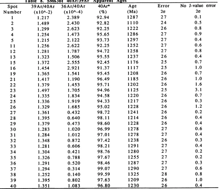
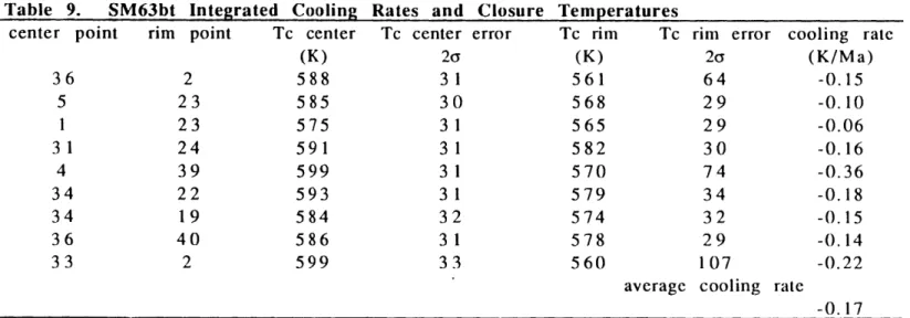
SM63bt

SM63bt is a biotite sample from a sample of main phase Sandia granite

from Embudito canyon (Figure A). SM63bt is 2.4 mm long and 1.8 mm wide.

Apparent

Ar/

Ar ages range from 1325 + 28 to 1110 + 24 Ma (Figure E). This

crystal has a "ridge" of older ages in with ages decreasing as one moves away

from this central ridge. Perhaps this is an artifact of breakage during

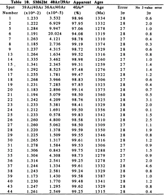
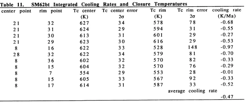
SM62bt

SM62bt is a biotite crystal from a sample of main phase Sandia granite

from Embudo canyon (see Figure A). SM62bt is 2.6 mm long and 2.1 mm wide.

The laser mapping revealed apparent 4 0_Ar/3 9_{Ar ages ranging from 1387 + 29}

Ma to 1230 + 26 Ma (Figure F). The average integrated cooling rate is -0.49

K/Ma.

3.6 Discussion and Suggestions

for Further Study

The age gradients found in these samples by 4 0_Ar/3 9_{Ar microprobe}

mapping, are not generally smooth, perfectly concentric in nature, or

centered relative to the edges of the crystal. If we assume these gradients are

generated by thermally activated diffusion, they have irregularities that

require some explanation. Detailed age mapping by Hames and Hodges (1993)

and Hodges et al. (1994) revealed troughs of younger ages in other slowly

cooled samples. These were interpreted to be fast diffusion paths with in the

crystal lattice. In one case, these fast diffusion paths formed a 1200 angle,

highly suggestive that, at least in this case, the fast diffusion paths were

subgrain boundaries related to cleavages. In this study, high-precision

mapping was sacrificed in the interest of analyzing as many different samples

as possible. It seems possible that some of the irregularities in the age

gradients may be due to fast diffusion paths, but I feel that drawing detailed

topographic maps of age gradients would require over-interpretation of the

available data for these samples, and therefore inappropriate.

The variety in the youngest apparent ages is strongly suggestive that

the age gradients are not due to episodic loss of argon by reheating. When a

free surface (edge of the grain) loses virtually all of the diffusing substance

present. Thus, a mineral which experienced this sort' of loss of radiogenic

argon, the youngest apparent age near the rim should provide a maximum

estimate of the timing of the reheating event. For argon gradients in the

Sandia samples to be formed by reheating, there would need to be thermal

pulses at -1331 Ma, -1296 Ma, -1230 Ma, -1110 Ma, and -790 Ma, if we assume

these samples are relatively intact. Due to absence of evidence for five

appropriately aged heat sources, the episodic loss hypothesis is extremely

unlikely.

The episodic loss hypothesis is also unlikely due to the disparity of

youngest apparent age for SM32mu (1331 Ma) and SM33bt (790 Ma). In order

for these gradients to be developed by reheating, it would require two thermal

pulses. The second pulse would need to be sufficient to reset SM33bt to 790 Ma,

yet cool enough and brief enough, to have no effect on the argon in SM32mu,

collected a mere 3m from SM33bt.

When the closure temperatures and cooling rates are plotted versus

apparent ages for all calculations for all samples, a remarkably coherent

curve is obtained (Figure most excellent). As reported in section 2.5, argon gradients developed by cooling histories that are not linear in T-1, can still

provide an integrated cooling rate that is tangential to the cooling curve at the

transitional temperature range. Different minerals record different portions

of the cooling curve due to the variability in closure temperature. The closure

temperature range is highly dependent on the size of the grain and diffusion

parameters. A variety of grain sizes and minerals can collectively define a

cooling curve by approximating different portions of the curve. Therefore

cooling path, than SM33bt, a smaller biotite grain. The coherence of the

cooling curve in Figure most excellent suggests that the five samples from the

Sandia pluton are collectively approximating the cooling history of the Sandia

pluton. If we assume that Figure most excellent represents a portion of the

cooling history of the Sandia pluton, the Sandia pluton experienced a thermal

pulse most likely associated with its intrusion and crystallization. After this

transient thermal spike, the plutonic samples record an episode of stable,

protracted slow cooling.

It is possible that age gradients could be formed due to chemical zoning

within a crystal. If there is an initial potassium gradient, there will a

production gradient for radiogenic argon. If the sample cools very rapidly, a

radiogenic argon gradient will be preserved due to the initial potassium

gradient, yet there will be no apparent age gradient, because the radiogenic

argon will be supported by a proportional potassium gradient. If there is an

initial gradient with a higher concentration of potassium in the center of the

grain, there will be higher radiogenic production in towards the center of the

grain. If we assume for the purposes of this thought experiment that no argon is lost from the system, the argon gradient will drive diffusion of argon until

there is a uniform distribution of argon. An apparent age gradient will exist

with older ages towards the rim, where argon produced in the

high-production (potassium-rich) areas has flowed into lower-high-production

(potassium-poor) areas. There will be younger apparent ages towards the

center of the grain where argon produced in this region has diffused towards

lower concentration region. In a situation where there is an initial potassium

gradient that is elevated at the edges, the radiogenically produced argon will

apparent ages in the center of the grain, progressively younger edges towards

the rim.

Research by Harrison et al, (1985) indicates some compositional control

on the diffusivity of argon in biotite. The diffusivity of argon increases with

increasing Fe/Fe+Mg content. I would predict that biotite grain with lower

Fe/Fe+Mg in the center of a grain and Fe/Fe+Mg towards the rim, will tend to

have older ages in the Fe-poor zones, and younger ages in the Fe-rich edges,

than a grain with an intermediate, homogeneous composition, all other things

being equal. In the reverse situation, a grain with Fe-rich core I would expect

the argon gradient to have a flatter morphology. The ages near the rims would

most likely be older than in an intermediate, homogeneous grain. The low

diffusivity of the rims would limit the escape of argon from the center of the

grain, creating an argon gradient with little topography. Thus, when

applying Dodson's method for calculating integrated cooling rates, a biotite

with a Fe-rich center may give anomalously rapid cooling rates, and a biotite

crystal with Fe-rich rims would tend to give anomalously slow cooling rates,

These predictions for the effect of composition could easily be checked by

running a number of finite difference models for the diffusion equation,

where the diffusivity would vary with position, or the amount of radiogenic

argon produced during each time step would vary with position.

In order to eliminate the possibility that gradients have been effected

by chemical variations within mineral grains, it will be necessary to do

microprobe analysis on samples from the Sandia pluton.

Another issue that should be considered is the effect of the increasing

concentration of vacancies in the potassium site. While a mineral is in

potassium site every time a potassium atom decays to radiogenic argon, which

in turn diffuses out of the system. The concentration ratio of

radiogenic/diffusion produced potassium-vacancies to originally filled

potassium-sites can be calculated by using,

D

1-

No

Where D is the amount of daughter isotope produced after crystallization and

prior to the time recorded by the apparent age. By definition, this quantity of

daughter product must be lost to the environment to obtain an apparent age

different from the crystallization age. For every daughter product lost to the

environment, a vacancy is produced in a potassium site. The value D/No is most

likely not the absolute concentration of vacancies at the time of closure.

During crystallization there are probably some vacancies formed in the

crystal structure as point defects. The concentration of these initial vacancies

are described in simpler physical systems in terms of an equilibrium

concentration of vacancies that minimizes the entropy of the system at a

particular temperature. For a complex process such as the formation of biotite

from a magma melt, calculation of the equilibrium concentration of vacancies

in the potassium site is non-trivial. The term D/No gives the additional

vacancies created over time beyond this initial concentration of vacancies.

The situation is complicated by the fact that vacancies can diffuse through a

substance and be lost at the surface of a system, when the concentration

within the grain is higher than the equilibrium concentration for a given

temperature. I know of no estimates for the diffusivity of potassium-site

vacancies in micas, but if we assume that the diffusivity of

potassium-vacancies is slower than the diffusion of argon, over time a significant

number of potassium-vacancies could be produced in the crystal lattice. For

example, if we assume that sample SM33bt crystallized at 1450 Ma, by the time

the center of the grain exhibits closed behavior at 1223 Ma, 10% of the

potassium atoms have decayed to argon and then diffused out of the mineral.

By the time the rim exhibits closed behavior, 30% of the original potassium

atoms have undergone radioactive decay, and the produced argon has escaped

the system. We might then expect the center of the grain to have at least 10%

of the potassium sites vacant, and the rim of the crystal to have at least 30% of

these site vacant. The atomistic process by which argon diffuses out of a mica

crystal lattice is not well understood. Given a cylindrical diffusion geometry,

this may be accomplished by a vacancy mechanism, in which an argon atom

would move through the crystal lattice by jumping into an adjacent

unoccupied site. Intuitively, if argon diffuses by jumping from potassium-site

to potassium-site, the greater the concentration of potassium-site-vacancies,

the easier it would be for argon to diffuse through the system. If there is a

strong correlation between potassium-site vacancies and the diffusivity of

argon in micas, the difference between 10% and 30% vacant potassium may

have a significant effect on diffusivity within the grain, and therefore on

closure temperatures. For SM33bt, the points at 1223 Ma and 790 Ma yield an

integrated cooling rate of -- 0.06 K/Ma, with closure temperatures of 584 K and

559 K respectively. This calculation assumes that the diffusivity of argon is

constant throughout the grain, varying uniformly only with the temperature

of the system. Let's assume the diffusion constants used to estimate the

integrated cooling rate are correct for the center of the grain, and we assume

the higher vacancy concentration near the rim increases the diffusivity, the

estimate of a closure temperature for the point at the rim may be too high.

Therefore, the cooling rate, in this situation, may appear slower than it

Chapter 4

Conclusions

The principal conclusions of this study are:

(1) Dodson's (1986) equations can predict, with reasonable accuracy, closure

temperature profiles for slowly cooled samples which experience cooling

paths that are not linear with T- 1

(2) Integrated cooling rates, found by using Dodson's (1986) equations, provide

a linear approximation of the cooling curve at the transitional temperature

range. The linear approximation is good even when the cooling history is not

linear with T- 1

(3) Different portions of a cooling curve can be approximated by analyzing a

suite of minerals with different transitional temperature ranges. A collection

of integrated cooling rates can define a portion of a cooling history.

(4) The thermal history of the Sandia pluton of New Mexico experienced a

transient thermal pulse related to emplacement and crystallization, followed

by protracted slow cooling. The cooling history obtained for the Sandia pluton,

when considered with the results from the Crazy Basin monzogranite (Hodges

et al., 1994), provide strong evidence for regional slow cooling at shallow