Bending vibration of rotating drill strings

(1)

Bending Vibration of Rotating

Drill Strings

by

I~.ong-Juin Shyu

rJ. S., Nati()n a I (~heng-I(IIng lJnivf'rsit y,

'ra

inall, '1'ai\vaII

( 1980)

1\1. S., National 'l'ai\van lJnivcrsity, 'raipei, 'raiv,ian

(1982)

Sllbnlitted in Partial FIIlfilJlrlent of tile R.eqllirelnents for tll~

Degree of

Doctor of Pllilosophy in Ocean Erlgin(~ering

at the

Massachusetts Institute of Technology

August 1989

©l\1assachusetts Institute of Technology,

1989

Signature of Author _

D(~partment of Ocpan 11:n~iTlcerillg

AllgllSt. 7, JDHD

C;crtificd by . V_V-...""_F...'-V_.V_""""_-_-_· _

/ _})rofcssor _.1. _KiTTl _Vandiver

Thesis Supervisor : I MASSACHUSEnS INSTillJTE OfTfC!-J'.· ;¥ A ccepted by ---.L.._--'IIIl..c==~---=:::.sllL.___ _~-===___ ~--+'----_--,-- -=<::::::J

Professor A. Douglas Carmichael Chairman, Departmental Graduate Comrnittee ,.~

0 V

17 1989

(2)

Bending Vibration of Rotating Drill Strings

by

Rong-Juin Shyu Submitted to the

Department of Ocean Engineering

un August 4, 1989 in partial fulfillment of the requirements for the Degree of Doctor of Philosophy

Abstl"act

Several domirlant mechanisms which cause the bending vibration of rotating drill strings have been identified, they a.re :

• Linear coupling between d}"namic axial force and bending vibration • Parametrically excited bending vibration due to dynamic axial force • Whirling of the drill string with and without borehole contact

Mathematical models for explaining and predicting these bending behaviors have been found and discussed. Experiments carried out in the laboratory confirmed tIle existence of the linear and parametric coupling between axial force and bending vi-bration. Data from a field test conducted in 1984 by Shell Oil Company also showed the existence of the both types of coupling. Forward and backward whirling of the drill string are also evident in this data set.

Because of the effect of rotation, the frequencies needed to excite the linearly coupled bending vibrations, and the parametrically excited bending vibration, are varying linearly with respect to the rotational speed. This phenomenon is explained and demonstrated by the laLoratory experiments. The effect of rotation plays a crucial role in understanding the bending vibration of a rotating drill string.

Thesis Supervisor: Professor J. Kim Vandiver Title: Professor of Ocean Engineering

(3)

Acknowledgments

I would, first of all, like to thank my academic and thesis advisor, Prof. J. Kim Vandiver, for his helpful insights that lead me to this thesis topic, for his patience and guidance that made this thesis possible, and for his great personality that made my stay in MIT very fruitful and enjoyable. I would like to thank my thesis committee: Prof. Stephen Crandall, Prof. Dale Karr, and Dr. George Triantafyllou, for their critical suggestions that help in writing this thesis.

My special thanks go to my family, especially my parents, for their continuing encouragement and support over the years. I would also like to thank my colleagues over the years, C. Y. Liou, T. Y. Chung, N. Joglekar, H. Y. Lee, C. Y. Hsin, Chifang Chen, H. Miyachi, for their numerous discussions and friendship. I would also like to thank Ms. Shiela McNary for her many typing jobs.

This work is primarily sponsored by Agip, Amoco, Annadrill, Britoil-BritiGh Petroleum, Elf Aquitaine, Exploration Logging, Exxon, Shell, Statoil, Teleco, and Total. A spe-cial thanks goes to Shell Development Co. for the permission to publish data which were acquired during a field test in 1984.

Finally, my thanks goes to two special friendsr my master's thesis advisor, Prof.

C. S. Lee of National Taiwan University, and Ms. Chou Su, for their friendship and encouragement which have positively changed many aspects of my life.

(4)

30 18 18 19 24

49

50 53

(5)

4.4 Bending Vibration of the BHA With Parametric Excitation Without Wall Contact . . . 54

4.5 Equation of Motion . . . 54

4.6 String under Dynamic Axial Tension . . . 58 4.7 Equation of Motion in a. Rotating Coordinate System 60 4.8 Parametric Excitation of Bending Vibration a With Borehole

Con-straint a • • • • • • • • • • • • • • • • • • • • • • • • • • • • • • • • • • • 61

5 Rubbing of the Drill Collars 5.1 Kinematics of Whirling . .

5.2 Partial Rubs .

5.3 Forward Synchronous Rub . .

5.4 Backward Whirl with Wall Contact. 6 Laboratory Experiments

6.1 Dimensional Analysis. . 6.2 .Model Selection . . . . . 6.3 Setup of the Experiment .

6.4 Data Acquisition . . . . 6.5 Experimental Procedures

6.6 Discussion of the Results . .

67 69 70 71

74

19 79 82 82 85 85 87 7 Field Tests 103 7.1 B a c k g r o u n d . . . 103 7.2 Data Processing 104

7.3 Case Studies of the Bending Vibration and Whirling Motion. 105

7.3.1 Bending Moment Measurements 106

7.3.2 Dl~lling Case Studies. . . 110 7.3.3 Case 1: No Whirl An~ Simple Rotation of a Curved Drill Collar. III 7.3.4 Case 2: Forward Synchronous Whirl w

=

n . . .

111 7.3.5 Case 3: Backward Whirl With Little Slip . . . 113 7.3.6 Case 4: Backward Whirl With Substa.l1tial Slip . . . 116 7.3.7 Case 5: Linear Coupling of Axial and Transverse Vibrations. . 121

7.3.8 Case 6: Parametric Excited Bending Vibration . . . 124

8 Conclusions and Suggestions 1~7

A Finite Difference ForlDulatloDs for Linear Bending Vibration 135 B Equations of Bending Vibration with Borehol~Constraint 141

(6)

C Green Function of 8 Rotating Beam with Linearly Varying Tension143

C.l Green's Function · . . . 144

(7)

List of Figures

1.1 A Typical Oil DriHing Rig .

..

12

1.2 Bottom Hole Assembly . 13

1.3 A Four-Bladed Stabilizer. 14

1.4 Stress Variation Along the Drill String 15

21 23 21 23 19 20 24 25 27 32 32 2.1 Definition of the Coordinate System .

2.2 Tangential Velocity of a Circumferential Point vs Whirling SpQed 2.3 Backward "'hirl with Slip, Rotation Speed -2.2 Hz, Whirlink Speed 9.9

Hz ~ · .

2.4 Backward Whirl, No Slip, Rotation Speed -2.2 Hz, Whirling Speed 8.8

Hz I • • •

2.5 Backward Whirl With Forward Slip, Rotation Speed -2.2 Hz, \'Vllirling Speed 2.2 Hz . . . 22 2.6 No Whirl, Pure Rotation, Rotation Speed -2.2 Hz, Whirling S;>eed 0 Hz 22 2.7 Forward Whirl With Slip, Rotation Speed -2.2 Hz, Whirling Speed -1.1

Hz " .

2.8 Synchronous Whirl With Slip, Ro~ationSpeed -2.2 Hz, \Vhirling Speed

-2.2 Hz , .

2.9 .Forward Whirl With Forward Slip, Rotation Speed -2.2 Hz, Whirli.lg

Speed -3.3 Hz .

2.10 Points on the Drill Collar .

2.11 Whirl Deflected Shape .

2.12 Motion Seen From the Fixed Coordinate System . 2.13 Motion Seen from the Rotating Coordinate System. 3.1 3.2 3.3 3.4 3.5 3.6

3.7

Several Configurations of the BHA BHA Near the Bit . . . . Coordinate System . . . .

Discretization of the Drill Collar . . . . . Viscosity of Drilling Muds . . . . First Two Bending Modes . . . . The Effect of WOB on Natural Frequency . . . .

34 36

37

38 40

42

7

(8)

3.8 The Effect of TOB on Natural Frequency . . " 3.9 Frequencies Observed in a Rotating Coordinat'e 3.10 Mass-Spring System on a Rotating Table

43 45 45 4.1 4.2 4.3 4.4 4.5 4.6 4.7 4.8 4.9 4.10 5.1 5.2 5.3 5.4 5.5 5.6 6.1 6.2 6.3 6.4 6.5 6.6 6.7 6.8 6.9 6.10 6.11 6.12 6.13 6.14 6.15 6.16 6.17 6.18

A Section of a Bent Collar . . . . Drill String Model for the Linear Coupled Example. The Effect of the Curvature on the Natural Frequencies Drill Collar Under Axial Excitation . .

Region of Parametric Instability . . . String under Axial dynamic Tension . . . .

Region of Parametric Instability With Rotation Rate 2.4 Hz .

Coordinate System .

Inputs for the Severity Calculation . . . . . Severity versus Frequency Plot

A \Vhirling Drill Collar .

The Displacement at Quarter Length and Half Length above the Bit .

A Vertically Mounted Rotor Model .

Force Diagram of Backward Rubbing ~ .

Time Domain Integration, With Initial Whirl Ratio -0.25, and 0.25 . . Time Domain Integration, With Initial Whirl Ratio 0.25, and Addi-tional Wall Reaction . . . .

Layout of the Experiment

The Location of the Stra in Gages . Signal Path of the Experiment . Force Spectra, Non-Rotating .

Bending y' Spectra, Non-Rotating, Parametric Resonance Cascade of Force Spectra, Rotating at 2.5 Hz . . . .

Cascade of x' Bending Spectra, Rotating Clockwise at 2.5 Hz . . . Bending x' versus Bending y', foz

=

1.2 Hz .

Bending x' and Bending y' Time History, foz = 1.2 Hz . Bending Magnitude and

Phase,

foz = 1.2 Hz .

Bending x' versus Bending y',

loz

=

6.0 Hz . Bending x' and Bending y' Time History, !o~

=

6.0 Hz . . Bending Magnitude and Phase, f.z

=

6.0 Hz . Bending x' versus Bending y',

laz

= 7.1 Hz . Bending x' and Bending y' Time History, fQ& = 7.1 Hz . Bending Magnitude and Phase,

faz

= 7.1 Hz . Bending x' versus Bending y', f(J~ = 12.6

Hz. . . .

Bending x' and Bending y' Time History, faz

=

12.6 Hz

8 50 52 52 55 59 59 61 62 66 66 68 73 74 75 77 78 83 84 86 89 90 95 96 96 97 97 98 98 99 99 100 100 101 101

(9)

7.1 7.2 7.3 7.4 7.5

6.19 Bending Magnitude and Phase, fQ% = 12.6 Hz ·

Top View of the Sensor Package. . . . .. . .. .. .. . .. .. . Whirling Drill Collar . . .. . .. . . .. . . .. . . Cross Section of Borehole and Whirling Drill Collar . . . .

Coordinate System, Bending Moment, and Phase Angle Definition Time History of the Bending Moments for Case 1: No Whirl, Pure

Rotation ..

7.6 Time History of Unwrapped Phase Angle for Case 1: No Whirl, Pure

"Rotation ..

7.7 Bending Moment Spectra for Case 1: No Whirl, Pure Rotation . 7.8 Time History of Bending Moments for Case 2: Forward Synchronous

Whirl c Of .

7.9 Time History of Phase Angle for Case 2: Forward Synchronous Whirl 7.10 Bending Moment Spectra for Case 2: Forward Synchronous Whirl . . 7.11 Time History of Bending Moments for Case 3: Backward Whirl with

Little Slip, s

==

.75 Of .

7.12 Time History of Phase Angle for Case 3: Backward Whirl with Little

Slip, s = .75 .

7.13 Bending Moment Spectra for Case 3: Backward Whirl with Little Slip,

5

=

.75 .

7.14 Orbital Plots of Bending Moments for Case 3: Backward Whirl with Little Slip, s = .75 . . . .. . . .. . . 7.15 Time History of Bending Moments for Case 4: Backward Whirl with

Substantial Slip, s = .58 .

7.16 Time History of Phase Angle for Case 4: Backward Whirl with Sub-stantial Slip,s = .58 . . . . 7.17 Bending Moment Spectra for Case 4: Backward Whirl with Substantial

Slip, s

=

.58 . . . . 7.18 Time Histories of Weight on Bit and Bending Moment for Case 5:

Linear Coupling Between Axial Force and Bending Vibration . . . . . 7.19 WOB and Bending Moment Spectra for Case 5: Linear Coupling

Be-tween Axial Force and Bending Vibration . . Of • • • • • • • • • • • • •

7.20 Coherence and Cross Spectrum Phase Between Axial Force and the x

Component of Bending Moment .

7.21 WOB Spectrum for Case 6 .

7.22 Bending x' and Bendingy' Spectrum for Case 6. . . . 7.23 Linear and Quadratic Coherence Between WOB and Bending x for

Case 6 .

A.I The Fictitious Point for the Finite Difference Scheme.

9 102 104 106 107 108 112 112 113 114 114 115 1]7 117 118 118 119 120 120 122 123 123 125 126 126 136

(10)

List

pf

Tables

2.1 Rotation Rate, Whirl Rate, and Slip Velocity . . . 28 3.1 Added Mass Coefficient of a Vibrating Rod in a Confined hole 39

3.2 BEND2PC Sample Input Data 41

5.1 Inputs for the Example . . . . 72

A.I The Finite Difference Matrix for a Two Spans Drill Collar . . .

10

(11)

Chapter

1 Introduction

The vibration of drillstrings includes longitudinal, torsional and bending vibration. This dissertation focuses on bending vibrations in the bottom hole assembly (BHA). The BHA is emphasized because many of the the most severe forms of bending vi-bration OCCUI' there, and because the most common location for drillstring failures

attributable to bending vibration is in the BHA. Bending vibration is often severe near the bit, because bit forces drive some forms of bending vibration. Whirling is also most common near the bit, because the large mean compressive loads on the drill collars near the bit produce significant curvature of the drill collars.

Bending vibration generated near the bit does not usually propagate to the surface as torsional and longitudinal vibration does. This is due to the vastly different wave propagation velocities. The propagation speed of axial waves in steel drill pipe is about 16,850 feet per second and of torsional waves is about 10,200 ft/sec. Even at a depth of several thousand feet the distance to the bottom of the hole is no more than a few wave lengths at frequencies less than 30 Hz. Thus these waves are commonly felt at the surface. In contrast bending waves at 30 Hz have a wave speed ofapproximately600 ft/sec, andtherefore must travel manywavelengths to reach the surface. Lower frequencies travel even more slowly. Furthermore, bending vibrations have larger damping, produced by the mud and wall contact and therefore, bending waves, generated at the bottom do not propagate to the surface unless the hole is very shallow.

(12)

_ _ _ _ _ _ _ _ _ _ _ _ Chapter 1 page 12

Engine House

~tud Pump Mud Pit

Drilling Line

Derrick

J<6IIII~-- Traveling Block

...- - Swivel •. . - - - - 4 + - - K elly

Rotatory Table

Mudmoving upward Drill Pipe

~1ud moving downward ---...

..

via driJ) stem

Drill Collar

+--- Bit

Figure 1.1: A Typical Oil Drilling Rig

In part, because bending vibration was not commonly observed at the surface, it was not wellunderstood orrecognized as being a problem. Theevidence of connection fatigue failures in drill collars, failure of downhole MWD tools and heavy surface abrasion of collars anti stabilizers has provided evidence to the contrary. In recent years, the availability of downhole vibration measurementshas provided the necessary insight to guide the development of bending vibration models for BHA's. The goal of this dissertation is to identify and describe the most important bending mechanisms in BHA '8, to develop analytical and numerical models of these phenomena and to verify them through the use of laboratory models and downhole measurements.

1.1 Basic Drilling Equipment

Let us start by int:-oducing the terminology for drilling frequently used in a drilling operation.

J'-

typical land-based drilling rig is shown in figure 1.1 There are several

(13)

_ _ _ _ _ _ _ _ _ _ _ _ Chapter 1 BI-IA Bit - - - -... page 13 Drill pipe About 30 Des

Figure 1.2: Bottom Hole Assembly

terms that are used frequently in the drilling industry and in this thesis. Following is a list of these terms.

Drill String: It consists of the kelly, drill pipe, drill collars, and a variety of special tools. Either collar or pipe can be added to extend the drilling depth.

Drill Collar: Drill collars are designed to operate in compression without buck-ling, so as to provide the weight and torque to the bit.

Drill Pipe: Drill pipe is used to transfer torque from the rotary table to the drill collar and to support the weight of the drill string. Drill pipe is designed to operate in tension, so the cross sectional area is smaller than that of the drill collars.

Bottom Hole Assembly (BHA) : It is a section of the drill string from bit to the top of the drill collar. Its length is typ!cally several hundred feet. Fig 1.2 shows the BHA.

Stabilizer: It is a device that holds the drill collar in the center of the borehole. The arrangement of the stabilize}'!; affects the direction of the borehole and the bending natural frequencies of the drill collars. Fig 1.3shows a standard four-bladed stabilizer.

(14)

Figure 1.3: A Four-Bladed Stabilizer

Weight On Bit (WOH): The compression force acting on the bit. Torque On Bit (TOB): The torque acting on the bit.

1.2 Problems in Drilling Dynamics

The dynamics of a drill string pose a unique problem in vibration analysis. In the upper part of the drill string, the state of the stress is tension, whereas, in the lower part of the drill string due to the weight on the bit, the state of the stress is compression. Figure 1.4 depicts typical stress variations along the drill string. A drill string is also subjected to various dynamic forces, including:

1. mud pressure fluctuations

2. weight on bit and torque on bit fluctuations 3. internal and external damping forces

4. centrifugal forces.

(15)

_ _- - - Chapter 1 page 15

Drill String

- . - - Compression

Bit

Rig

...--..a.--...- ... . . . - - - Soi I Surface

Tension

t

WOB (weight on bit)

Figure 1.4: Stress Varia.tion Along the Drill String

Because of these forces, a number of problems may arise. For example: the bit may bounce on the cutting surface resulting in bit damage; severe bending moments may develop in the BHA leading to the fatigue failures; forward whirl may cause wear against the bore hole, and backward whirl due to the friction of the wall may result in fatigue failure. These phenomena are all hazardous to drilling operations.

1.3 Outline of the Thesis

This thesis concentrates on the understanding of bending related vibrations of the BHA. They include whirl-related motion, bending vibration due to linear coupling with axial forces, and parametrically excited bending vibration. These studies will

(16)

_ _ _ _ _ _ _ _ _ _ _ _ _ Chapter 1 page 16 help us gain insights into the dynamic behavior of the BHAs.

In the second chapter, the motions of a typical drill collar are described in both fixed and rotating coordinate systems. These motions include forward whirling , backward whirling, and whirling with bending vibration. Detail is given to reveal how one uses measurements made in a rotating frame of reference to deduce the collar motions. The rotating frame of reference is important to drilling engineers, since most downhole transducers are mounted inside rotating drill collars.

In the third chapter, the equations of motion of bending vibration of the Bottom Hole Assembly are given, and a finite difference scheme is introduced to solve the eigenvalue problem. This model accounts for the effects of linear varying compres-sion, mud added mass and damping forces, and dynamic variations ill WOH. It also takes into account the effect of stabilizers. The natural frequencies are expressed with respect to a fixed coorciinate system. The bifurcation of the natural frequencies re-sulting from expressing natural fre:}uencies in terms of a rotating coordinate system is also explained.

In the fourth chapter, linearized coupled equations between axial and bending vibration are presented by assuming small curvature. This equation represents the lineareff2ct of axial force on the bending vibration. Also presented are the equations of motion showing the parametric axial force excitation of bending vibration. Examples are given to demonstrate linear and parametric axial excitation of bending vibration. In the fifth chapter, rubbing contact between the drill collars and the wall are explained. Forward and backward whirl with slip are presented. Whirling can poten-tially shorten the fatigue life of drill collars and can cause substantial surface abrasion. Chapter six shows a series of laboratory experiments that demonstrate the be-havior predicted by the mathematical model. The experiments included strain gage bendingmeasurementsof whirling and bending vibration. Linear and parametric cou-pling between axial force and bending viblation are demonstrated in both rotating and non-rotating cases.

(17)

Chapter seven shows the results of a field test. This test was conducted by Shell._. and NL in 1984. A total of 60 hours of downhole data were taken during that experi-ment. Six examples are presented to demonstrate the behavior mentioned in previous chapters, including, whirl, linear coupling, and parametrically excited bending vibra-tion.

Chapter eight concludes th~ results obtained 80 far. Several suggestions are made for future research.

(18)

Chapter

2 Measurem.ent System.s on a

Rotating Shaft

In rotor vibration measurements, the motion of the shaft is usually measured by proximity probes. This kind of measurement reveals only the motion of the center of gravity of the shaft. The measurements are taken with respect to a fixed coordinate system, att.ached to the earth. When the measurements are taken by a transducer attached to the rotating shaft, they are more difficult to interpret, because they are not taken with regard to a fixed coordinate system, and usually are not taken at the center of gravity. The following gives a simple description of the motion of a drill collar as seen from both frames of reference under various combinations of whirling and rotation, and shows how to interpret'the measurements from transducers attached to the collar.

2.1 Motion of a Drill Collar in Pure Whirling

Figure 2.1 is the definition of the coordinate system used to describe the motion of the drill collar, where :

Oxy = fixed reference frame centered in the borehole

Ox'y'

=

rotating reference frame with speed

n

and with its origin located on the axis of the borehole

Ax"y"

=

rotating reference frame with speed w and with origin 18

(19)

. Chapter 2 y - - - page 19 Drill Collar x Borehole

Figure 2.1: Definition of the Coordinate System located at the center of the drill collar

n

=

whirling speed ofthe collar with respect to Oxy (rad/sec)

w

=

rotation speed of the collar with respect to Oxy (rad/sec)

R1 = whirling radius or displacement of the drill collar center

R2 = radius of the collar (= 3.5 inches in examples)

R_s

=

radial location of the radial and tangential accelerometers

When the collar contacts the wall, R1 equals the clearance, which in these examples

is specified as .875 inches.

2.2 Motion Seen From Coordinate

Oxy

Figure 2.2 shows the linear relationship of t1 VB. whirl rate, 0 at a fixed rotation r&te, w, where tJ is the tangential contact velocity between the circumference of the

collar and the wall. The following figures represent the trajectory of a point P,

fixed

to the circumference of the collar, as seen from a

fixed

coordinate system, Oxy, under various slipping and whirling conditions. In all cases, the collar is in constant contact with the wall. Figures 2.3 to 2.9 correspond to the points a through g as shown on

(20)

_ _ _ _ _ _ _ _ _ _ _ _ Chapter 2 - - page 20 .!' V

•

'J I ••c~••'d Whlrt FOI ••,dWN,I i _•

..

~ Z

•

~ i

•

'.clr.••rd Whi,1

•

0 a

..

Witll 'Ii~ Z WNrl _I unli'el,

•

. v=RtO+ R₂(J) .1'11"

"""

...

,

11 b c d e f g

Figure 2.2: Tangential Velocity of a Circumferential Point VB Whirling Speed

Figure 2.2. Figure 2.8 represents the trajectory under synchronous whirl, in which whirl rate is equal to rotation rate. The minus sign of the rotation rate indicates the direction is clockwise. Figure 2.6 shows ttle trajectory of P with pure rotation, ie.

n

equals to zero. Figure 2.4 show the trajectory of point P under backward whirl with no slip. The backward whirl rate under this condition is

~~'

and the velocity at the contact point between the collar and the wall is always pointing toward the center of the hole. No tangential velocity component is present in this case. Figure , 2.5 shows the trajectory of P under backward whirl with slip. The backward whirl rate is smaller than that in Figure 2.4, and the tangential velocity of the contacting point is no longer zero. Figure 2.7 is the case of forward whirl with slip, but the whirl rate is lower than the rotation rate. Figure 2.3 represents the case when the backward whirl rate is larger than

~~'

and Figure 2.9 shows the case with forward whirl rate greater than the rotation rate. Both of these cases are not likely to happen in the real drilling situation. In all cases mentioned above, the ~enterof the collar, point At would appear to move in a circle about 0 with a radius

R

1 and at frequency

n .

(21)

_ _ _ _ _ _ _ _ _ _ _ _ _ Chapter 2 - - - page 21 4 5 2

o

INCHES ..2 2 4 -4 .5 ~--L-_ _- - £ - - -. . . . .- -...-_-...-.-J ~5 -4 ..2 INCHE

o

Figure 2.3: Backward Whirl with Slip, Rotation Speed -2.2 Hz, Whirling Speed 9.9 Hz 4 5 2

o

INCHES ..2

-s

I..-....J..._ _-.L_ _

--..L----..I---..---S -4 5---..-,---~---r----,r--, -4 -2 2 4 -INCHE

o

(22)

_ _ _ _ _ _ _ _ _ _ _ _ Chapter 2 - - - page 22 4 5 2

o

INCHES -5 ~-.&..._ __ _ L . ._ _--...L._ _--a._ _----t"""'-__ -5 -4 -4 -2 5 - - - ---.---.~.--. 2 4 INCHE

o

Figure 2.5: Backward Whirl With Forward Slip, Rotation Speed -2.2 Hz, Wllirling Speed 2.2 Hz 4 S 2

o

INCHES -2 2 5---.----.--.---,..---,r----y---, 4 -4 -2 -5 L..-...J.._ _--1._ _- . L ~ _ -...-.. -S -4 INCHE

o

(23)

4 5 2 o INCHES -5 L . . -..._ _- - - ' -_ _- . . . ._ _- - "_ _- - ' _ - ' -5 -4 -4 -2 5

..----...---r---.---r--_-__

2 4 INCHE

o

Figure 2.7: Forward Whirl With Slip, Rotation Speed -2.2 Hz, Whirling Speed -1.1 Hz 4 5 2

o

INCHES -2 2 5r-...,...---,---,..---r---.~_ 4 -2 -4 -5 '___--'-_ _..._ _..._ _---1._ _---..11...---1 -S -4 INCHE

o

Figure 2.8: Synchronous Whirl With Slip, Rotation Speed -2.2 Hz, Whirling Speed -2.2

Hz

(24)

4 5

2

~5 L--~_ _---a._--~---""'-'--'

~5 -4

o

INCHES

Figure 2.9: Forward Whirl With Forward Slip, Rotation Speed -2.2 Hz, Whirling Speed -3.3 Hz -4 lNCHE

o

2 4

2.3 Motion Seen From the Rotating Coordinate

System

Ox'y'

This coordinate system rotates at

n

about the center of the borehole, point O. In this coordinate system, the center of the collar, point A, would be at a distance R1

from 0 and would not move, as depicted in Figure 2.10. Any other fixed point, such as B or P, on the drill collar will appear to rotate at w -

n

in the rotating frame of reference about an apparent center displaced from 0 an amount equal to R1 • Figure

2.10 also shows the locus of two points B and P asseellfrom the Ory' rotating frame.

P is a point on the surface of the collar, and lies on an axis

r',

which rotates with the collar. This point appears to go in circles at a rate w - 0, with a radius R

_z•

Point B simulates the location of the accelerometers in the collar. They &!e not on the outer circumference of the collar, but are at a lesser distance from the center. That point, B, would appear to move as shown, also a circle with radius R

_a,

centered at R1 from

(25)

y" y'

XU

x'

Figure 2.10: Points on the Drill Collar collar.

2.4 Measurements Taken in a Rotating Reference

Frame Under Pure Whirl Condition

2.4.1 Bending Moments

B

x'

and

By'

Bending moments are determined by the curvature of the beam as computed with respect to the neutral axis. In this case, the neutral axis coincides with A, the center of the collar. The deflection of the collar center as seen in the rotating frame Ox'y' is designated

vo(z)

and is assumed to be given by :

(2.1)

vo(z) defines a radial distance from the borehole center(z axis) to the center of the

(26)

radial deflection of the collar center as a function of the distance, %, along the axis from

the bit, as shown in Figure 2.11. Here it has been assumed that the whirl deflected shape of the collar is half a sine wave between the bit ~d the first stabilizer. Figure 2.10 was drawn assuming one was at the midspan of the collar. At any other

z,

the distance to the center of the circle made by B and P would be given by R1sin(

¥) ,

and the radii of the circle R2 and Rs would not change. At the bit, fOlr example, the

points Band P as seen in the rotating frame Ox'y' would be circles centered at 0 and moving at an angular rate of w -

n.

The bending moment corresportding to

vo(z)

is given by the moment curvature relationship

(2.2)

In the examples drawn from the Shell-NL fields experinlents, the bending moment

B(z)

wasmeasured by twoperpendicularly mOlJnted strain gages in the Ax"y" system, which rotates with the collar. But note that

B(z)

is a two vector components in the Ax'y' syst~m,with unit vectors i' and j', because the strain gages measure the strain from the undeflected position, which is the center of the hole.

B(z)

=

B(z)[sin(w -

n)ti'

+

cos(w - O)tJ·']

=

B

z '

+

B

II,

(2.3)

In the example given, the distance, L, from the bit to the center of the stabilizer was 59~2 feet. The collar outside diameter was 7.0 inches, in an 8.375 inches hole. A midpoint deflection equal to a clearance of .875 inches would lead to a midpoint bending moment of3525 foot-pounds. In the Shell-NL tests, the strain gage location was typically nine feet above the bit. At the measurement location nine feet above the bit, the measured bending moment would be reduced to 1600 foot pounds. The bending moment measurement can be used directly to interpret the whirling motions of the collar. The magnitude of the bending moment is simply giv-en by

(27)

_ _ _ _ _ _ _ _ _ _ _ _ Chapter 2 - - - page 27 Stabilizer v(z) Bit z

1

L

Figure 2.11: Whirl Deflected Shape A phase angle can be estimated from Bz ' and BII , ;

BZI 1 sin(w - n)t

tP (t)

=

tan-1(-B ) = tan - ( n) = (w - n)t

~' cos w - t

(2.5)

tP(t)

is simply the phase angle which accumulates at the rotation speed of the collar as measured in the Ox'y' system. Therefore, from the bending moment measurements, the magnitude of the whirl can be estimated, and from the phase angle the difference between,whirl and rotation rate can be determined, but not unique values of wand O. In contrast, a magnetometer is insensitive to whirl and only sees the rotation of the collar with respect to the fixed reference frame. Its output is sensitive to the rotation rate w, but provides no information regarding the whirl rate

o.

Considerthe different whirling conditions described in Figure 2.2 The values ofw,

n,

and w -

n

are summarized in the following table for all cases a through g. Note for this particular table the relative contact velocity with the wall is also presented.

(2.6)

where R1

=

0.875 inches, R2=3.5 inches.

(28)

Table 2.1: Rotation Rate, Whirl Rate, and Slip Velocity

Case w/21f

n/21f

(w -

0)/211"

_I

_v

_I

a Backward whirl with slip -2.2 9.9 -12.1 .50

b Backward whirl, no slip -2.2 8.8 -11 0

c Backward whirl, forward slip -2.2 2.2 -4.4 3.02

d No whirl, pure rotation -2.2 0 -2.2 4.03

e Forward whirl with slip -2.2 -1.1 -1.1 4.53

f Synchronous whirl with slip -2.2 -2.2 0 5.04

g Forward whirl with forward slip -2.2 -3.3 1.1 5.54 where vis expressed in ftJsec. Note that in all cases ~=-2.2 Hz" where the minus sign indicates clockwise rotation looking down the hole(tuming to the right). This would be the frequency of the peak one would observe in a spectrum of a magnetometer output. H one were to compute a spectrum of the time history ofeither B_{z '} or B_II"

the peak would occur at the frequency

I

w -

n

I .

The total magnitude B does not vary with time. A polar plot of Band

¢(t)

would produce a circle with a radius B,

an angular velocity ofw - 0, and rotation angle

t/>(t)

equal to

(w -

O)t.

The phase rates w -

n

has a physical significance. It represents the frequency of bending stress cycles experienced by the collar. For example, synchronous whirl, case f in table 2.1, results in no bending fatigue. However, it has a relativel:r high tangential velocity and, therefore, would tend to abrasively wear out the culiar.. On ihe other hand, case b, backward whirl with no slip, has zero tangential veiocity and hence no wear. However, for this particular case the bending cycles would occur at approximately five times the rotation rate.

(29)

2.4.2 Acceleration Measurements with Radial and

Tangen-tially Mounted Accelerometers Fixed to

the Collar at

a Radius

R

_s

Accelerometers measure absolute acceleration regardless of reference frame. There-fore, a radially oriented accelerometer mounted at a radius R

s

from the collar center would respond to the radial acceleration, Raw2, with respect to the center of the collar,

as well as the component of the whirl acceleration of the collar center in the direction of the radially mounted accelerometer. This componentis given by R102 cos(w -

O)t.

A tangential accelerometer would not feel any centripetal acceleration du(, to the col-lar rotation, but would respond to the tangentially oriented component of the whirl acceleration of the collar center. Therefore, we may write

ar - R1

n

2cos(w -

n)t

+

Rsw2

at R1

n

2sinew -

O)t

(2.7a)

(2.7b) where ar is the radial acceleration, and ac is the tangential acceleration. If the

ac-celerometers are of the piezoelectric type, they can not measure constant acceleration components. Thus, the Rsw2 term of the radial acceleration would not be measured,

and the acceleration magnitude as measured would be

and the phase angle

1

~

=

(a~

+

a:)2

=

R102

(2.8)

<p(t)

=

tan-I

(tit)

=

(w -

O)t

(2.9)

a,

In

the case of synchronous whirl, w -

n

= 0 and both

a,(t)

and

a,(t)

would not vary with time. In that caset the output ofthe aecelerometers would be zero, due to the

low frequency limitations of piezoelectric accelerometers.

In

reality, the drill collar may exhibit dynamic behavior other than pure whirling motion as described thus far. For example, torsional vibration will lead to non-zero tangential acceleration.

In

(30)

_ _ _ _ _ _ _ _ _ _ _ _ Chapter 2 _ _page ₃₀ 4>(t)=(w-O)t and~ =0. Torsional vibration would introduce a tangential acceleration component _{R s}

¢.

Similarly, transient impacts with the wall would cause tangential and radial accelerations which are not as simple as cases of pure whirl. Bendin~data are in practice very difficult to interpret when non-whirling caused vibration occurs. An example is discussed in the next section.

2.5 Measurements Taken on a Rotating Frame With

Simultaneous Whirling and Bending Vibration

Rotation and mass eccentricity cause a shaft to whirl. The ampU:

·,ne

o~ .~' whirling depends on the eccentricity, and on the closeness of the Jotatlon SPC{ anlt

the bending natural frequencies of the shaft. The whirling amplitude grows larger as the rotation speed approaches one of the natural frequencies. But as the collar whirls, bending"vibrations can also be excited, for example, by lateral or axial dynamic forces. Depending on the reference frame, these motions may seem simple or very complex.

An observer in the fixed coordinate system describes synchronous whirl as a cir-cular motion of the shaft. But to an observer staying in the center of the coordinate system

OX'Y',

rotating at 0, whirl is just a constant deflection. Assume that in addi-tion to this constant deflecaddi-tion, the rota:ting observer also witnesses a simple circular motion of the center of the shaft about the constant deflection center. The equations describing the motion of the sha.ft center as seen by this person are:

x'{t) -

R

z 'coswnt

1I'{t) -

R,.

sinwnt

(2.10a) (2.10b)

where

Rz,

and

R"

are the amplitude of the bending vibration and Wn is the bending vibration frequency relative to the rotating coordinate system. The trajectory seen from a non-rotating reference frame is given by:

x(t) -

R

1

cos(wt)

+

R

z'

cos(wnt) cos(nt) -

R,.

sin(wnt)

sin(nt)

y(t) -

R1

sin(wt)

+

R~Jcos

(wnt)

sin(nt)

+

R"

sin(wnt)

cos(Ot)

(2.11a) (2.11b)

(31)

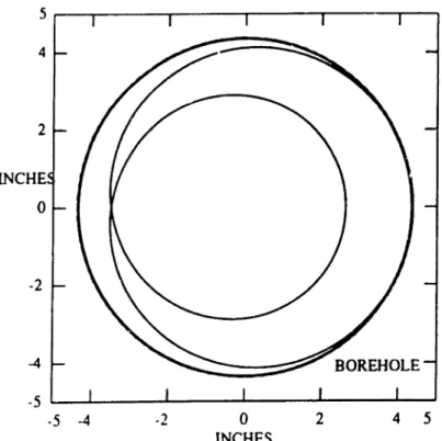
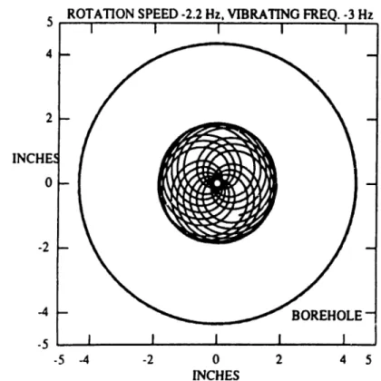
_ _ _ _ _ _ _ _ _ _ _ _ _ Chapter 2 page 31 Figures 2.12 and 2.13 give examples of the trajectories of the shaft center as seen from both rotating and non-rotating frame of references, assuming two dimensional bending motion as mentioned above. These figures are plotted with the following parameter values. The hole clearance is 88Sumed to be large enough that no wall contact occurs.

R

1

=

0.875 inches

Rz'

=

1.0 inches

RJlI

=

1.0 inches

n

= -2.2

Hz

= w, forward synchronous whirl

Wn = -3.0

Hz

The motion is circular with respect to the rotating coordinate system, but the ob-servers in the fixed coordinate system will see much more complicated motions. This example not only illustrates the differences in the appearance of the motion as seen in the fixed and moving frames, but also has a useful physical interpretation which will be illustrated in the experimental results. A whirling shaft excited by axial forces will respond with orbital motion superposed on the whirl motions just as in this example.

(32)

_ _ _ _ _ _ _ _ _ _ _ _ Chapter 2 - - - page 32 4 5 2

o

INCHES -2

.5 "__...Ao.o._ _- A o_ _-...I...-_ _ooI.-_ _...- J

-5 -4

5 ROTAnON SPEED -2.2Hz,VIBRATING FREQ. ·3Hz

-4 -2 2 4 INCHE

o

Figure 2.12: Motion Seen From the Fixed Coordinate System

5 ROTAnON SPEED -2.2 Hz, VIBRATING FREQ. -3 Hz

4 S 2

o

INCHES -2 2 4 -2 -4

-s

~-....

_ _

--..._-_a...-_ _..&.-_ _- ' - - J -5 -4 INCHE

o

(33)

Chapter

3 The Bending Natural Frequencies

of Rotating Drill Collars

The bending vibration of the BHA is less well understood than torsional or axial vibration. Relatively, few papers have been devoted to the study of this phenomenon. The lack of research is partly due to the fact that bendingvibrations downhole seldom propagate to the top, and to the lack of downhole measurements. Therefore, we begin with the discussion of the bendirlg vibration of the drill collars.

3.1 Basic Configurations of the BHA

The arrangement of the stabilizers in the BHA affects the direction of the borehole. Depending on the location of the stabilizers, BHAs can be categorized as building, holding, or dropping assemblies. Figure 3.1 shows five configurations of the BHA. Accordi~gto drilling practice, BHA no.1 is rated as a dropping assembly; BHA no.2 is found to be a very strong dropping assembly; BRA 00.3 is rated as a very strong building assembly; BRA no.4 is found to act as a good holding assembly; BHA no.5 can be used as a weak building or a weak dropping assembly, dependiIlg on hole geometry and the interaction between the stabilizer and the- formation. The placement of the stabilizers also affects the bending natural frequencies of the DBA. The simpliest approach, and the one taken here, is to model the effect of the bit and stabilizers with equivalent boundary conditions. Thus, a BRA is modelled as an axisymmetric,

(34)

bit

0

60'

g

30'

g

2

Og

90·

g

3 to' 30' 4

Og g

g

Og

30'

g

5

Figure 3.1: Several Configurations of the BHA

rotating, ~nultispan beam. The spans are determined by the placement of the bit and stabilizers. With this approach, BHA number 2 in Figure 3.1 might be modelled as a tv/o span beam that is hinged at the bit, restrained in displacement at the first .stabilizer. and given a displacement and moment spring restraint at the second stabilizer. Such a model, then, approximates the effect of the BRA above the second stabilizer by a simple spring. Depending on the value of the spring constant, this restraint can be varied from a simple hinged to a built-in (fixed) condition. This simple approach will provide estimates of the natU!al frequencies and mode shapes for bending vibration between the bit and the second stabilizer only.

(35)

(3.1)

3.2 Theoretical Background

Figure 3.2 shows a section of BHA near the bit. The coordinate systems for the drill collars are shown in Figure 3.3. The homogeneous governing equation for bending vibration for a rotating beam in the z direction is

[42]:

ApCMx

=

-EI::~

+

Q~~

-

(CE

+

C/

)%

+

CIWY

82

,;

ax

-ApghcostP[(l- z)

az

_{2 -}

az

J

+

ApCMaw

2

coswt

the !I direction is:

lJ4 y aSy

ApCMy =

-EI

az. -

Q

azs -

(CE

+

C/)y - C1wx

-Apghcos tP[(1 - z)

::~

-

:~)

+

ApCMbw2sinwt - ApghsintP (3.2)

if complex notation a' = x

+

iy and e' = a

+

ib are used, and dividing through by

ApCM , then

(3.3)

. The definition of each symbol is

A

=

cross sectional area of collar

p,Pm

=

density of steel and mud

GE,OI

=

external and internal damping

E I

=

flexural rigidity

9

=

gravity constant

tP

=

slant angle of drill collar

OM

=

mass coefficient of collar

=

l+(added mass of mud per unit length

+

· mud maos per unit length trapped inside the collar) / collar mass

(36)

_ _ _ _ _ _ _ _ _ _ _ _ Chapter 3 - - - page 36 Slant Mud Collar z

1..

Stabilizer Lb.OD2.1D2 Stabiliz.er La,ODI.IOl Bit

Figure 3.2: BHA Near the Bit

h

=

I_Pm p

1

=

weight on bit/Apghcost/>

Q

=

torque

w

=

rotation speed of the ·drill collar

e' = mass eccentricity of the collar

The undamped natural frequencies and mode shapes for the non-rotating drill collars may be sought by first setting the damping and rotating speed, w, to zero, and assuming static side force does not affect the natural frequency. The equations of motion can be expressed in a dimensionless form as follows. Let La = length of drill collar form the bit to the first stabilizer

w

-EI

w~ _- _ApCML:

z

La

(3.4a)

(3.4b)

(37)

Cros~ Section of a Drill Collar

y+b

)'

--+-...-x --+-...-x+a

OXY : fixed reference frame

x·

G gravity center C geometric center

(a.b) : eccentricity of the collar (i) rotation speed of the collar

OX'Y' : rotating reference frame

Figure 3.3: Coordinate System

T

-

wot (3.4c) s' (3.4d) s -La

11 -

I (3.4e) La then 82 8 848 .QL_G

aSs

gh coscP 828

as

a.,2

+

aw

4

+

I

EI

aw

s

+

LGCMW~

[(11 -

w) aw2- awl

=

0 (3.5)

By separating the time and spatial variables and using the central difference method to replace the spatial derivatives, the differential equation can be transformed into a system of algebraic equations. For details see Appendix A.

where

[D][s]

=

0

[D] is a n x n finite difference matrix

(38)

w=l+Lb/La w=l

w=o

j=N Stabilizer j=M Stabilizer j=2 j=1 j=O Bit

Figure 3.4: Discretization of the Drill Collar

(s] is a nx1 vector representing the non-dimensionalized displacements

The discretization of the collar is shown in Figure 3.4. The eigenvalues and eigenvec-tors ofthe matrix

[D]

are the natural frequencies and mode shapes of the non-rotating drill collar. The eigenvalue problem as described abovefor a two span beam has been implemented in a program known as BEND2PC.

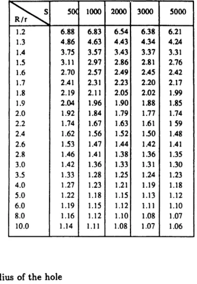
3.3 Added Mass Coefficient of a Rod in a Confined

Hole

The added mass coefficient of mud is a function of wall clearance and the vis-cosity of the mud [11]. Table 3.1 shows the added mass coefficient under various combinations of S and

Rlr,

where

S = wr2/v

(39)

Table 3.1: Added Mass Coefficient of a Vibrating Rod in a Confined hole

~

50< 1000 2000 3000 SOOO 1.2 6.88 6.83 6.54 6.38 6.21 1.3 4.86 4.63 4.43 4.34 4.24 1.4 3.75 3.57 3.43 3.37 3.31 1.5 3.11 2.97 2.86 2.81 2.76 1.6 2.70 2.51 2.49 2.45 2.42 1.7 2.41 2.31 2.23 2.20 2.11 1.8 2.19 2.11 2.05 2.02 1.99 1.9 2.04 1.96 1.90 1.88 1.85 2.0 1.92 1.84 1.19 1.71 1.14 2.2 1.74 1.67 1.63 1.61 1 59 2.4 1.62 1.56 1.52 1.50 1.48 2.6 1.53 1.47 1.44 1.42 1.41 2.8 1.46 1.41 1.38 1.36 1.35 3.0 1.42 1.36 1.33 1.31 1.30 3.5 1.33 1.28 1.25 1.24 1.23 4.0 1.27 1.23 1.21 1.19 1.18 5.0 1.22 1.18 1.15 1.13 1.12 6.0 1.19 1.15 1.12 1.11 1.10 8.0 1.16 1.12 1.10 1.08 1.07 10.0 1.14 1.11 1.08 1.07 1.06

R

=

radius of the hole

r

=

outer radius of the collar

w

=

vibration frequency in radians pe~second

The coefficients in Table 3.1 can also be obtained through following formula,

[0:~(1

+

"'1

2) -

8"'1] sinh(p - 0:)

+

20:(2 - "'1

+

"'1

2)

C08h(/1 - "'1) - 2"'1

2

[0:/1 -

20:~

0",

=

Re(

)

0:

2

(1 - "'1

2)

sinh(/1 - 0:) - 20:"'1(1

+

"'1) C08h(P - 0:)

+

2"'12

V;;P

+

20: ;

(40)

70 60 !I _,,~>,

.§

u

..

en

!

.s u ₅₀

=

en i§ 0 Q..

-

s:: 40 CJ u ~ 30 en 0 U en 20 > 10 0 8.3 8.7 9.1 9.5 9.9 10.3 10.7 11.1 Mud weight, ppg

Figure 3.5: Viscosity of Drilling Muds

where Re indicates the real part of a complex quantity, ex

=

kr,

P

=

kR, "y

=

~,

and k =

~.

Equation 3.7 is valid if both a and

P

are greater than 10. Figure 3.5 shows the viscosity for various drilling muds. To convert viscosity from centipoises to kinematic viscosity in

/t

2/sec, the following formula are needed.

poises= centipoises/lOO

p

=

mass densityof the mud

(slug/ItS)

v

=

kinematic viscosity

(ft

2

/

Bee)

=

poises/497p

3.4 Effects of WOB and TOB on the Bending

Vi-bration

A numerical example is given to show the effects of the WOB and TOB on the bending natural frequencies. The numbers used as the inputs to the program

(41)

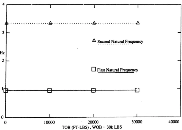
_ _ _ _ _ _ _ _ _ _ _ _ Chapter 3 - - - page 41 BEND2PC are shown in the Table 3.2. The first two modes are shown in Figure 3.6. Figure 3.7 shows the effect of the WOB and Figure 3.8 shows the effect of the TOB on the natural frequency of these modes. During Chilling operations, the WOB may reach SOK Ibs, but the TOB seldom exceeds 10,000 ft-lbs. So, from Figures 3.7 and 3.8,. we can conclude that the effect ofTOB on bending natural frequencies can usually be neglected. This assumption is made in chapter 4.

Table 3.2: BEND2PC Sample Input Data

59.8,35.23 (ll:bit to 1st stab. 12: 1st stab. to 2nd stab.,ft) 20,12 (no. ofsegments of II and 12)

6.83,2.93 (od and id of Il,inches) 6.25,2.81 (od and id of 12,inches)

o

(tab, ft-Ibs)

30000 (wob, lbs)

8.8 (mud density, lbs/gal)

5 (added mass coeff. of the mud)

1 (boundary condition at 2nd stabilizer.l=fixed O=depending on spring canst.)

o.

(slant angle of the borehole, degrees)

4.28e09,15.2(Young's Modulus and density of the collar,lbs/ft·*2,slug/ft**3)

o.

(boundary condition at bit,l=fixed O=depending on spring canst.) 0.,0. (moment spring constant at bit and stabilizer, ft-Ibs/rad)

The simplified fonnula shown below gives a rough estimate of the first bending natural frequency with WOB and TOB effects. This equation was obtained assuming constant axial force, T, and constant torque, Q,

Q2-4El+

T

WWOB,TOB

=

W

1 -

(3.8)

(42)

- - - Chapter 3 page 42

First Mode, 0.95 Hz

Second Mode, 3.33 Hz

Stabilizer

Bit

Figure 3.6: First Two Bending Modes

4---~---~---._----____,

···A ~ . ~ ~ 3 Hz 2

o

First NalW"alFrequency

o

L---.L---..L-.---..I..---40000~

o

10000 20000 30000

WOB(LBS)

(43)

_ _ _ _ _ _ _ _ _ _ _ _ Chapter 3 - - - page 43 4 , . . - - - -...- - - - . - - - . . . - - - . . , . - - - . . . , " ·A·

·A···l!J.

3 Hz 2

o

Firsl NaturalFrequency

4()(XX)

]ססoo 2()(xx) 3ססoo TOB (FT·LBS), WOB =30k LBS

OL....---~---...L---~---o

Figure 3.8: The Effect ofTOB on Natural Frequency

where WWOB,TOB, ware the natural frequencies with and without WOB and TOB

effects. Terif is the first critical buckling load of a pin-pin beam of length L, and

Q

is the torque. In actual drilling,

Q

seldom exceeds 10Kft-lb, so the quantity

4~I

is small compared to

T;

therefore, the effect of the torque can usually be neglected.

3.5 Natural Frequencies of a R,otating Beam

Ex-.pressed in a Rotating Coordinate System

Equation 3.3 describes the bending motion of a rotating beam with respect to a fixed reference frame. The bending vibration with respect to a reference frame ~otatingat speed w can be obtained by substituting

s

_-

r(w

_,,,\eiwf'_J

_(3.98.)

8 -

(r

+

iwr)e'c,,,·

(3.9b)

(44)

_ _ _ _ _ _ _ _ _ _ _ _ _ Chapter 3 - - - page 44 into equation 3.3, The resulting equation is :

, rOE

+

01 •

l.'

EI

a

4r' .

Q

a

1Jr'

r

+

ApC_M

+

12w r

+

ApCM

ai-

+

IAIlC

M

az

3

ghcosq,[(l )02r'

or']

(2

·

CEW ) "

2'

.ghsint/J -illJ"3

10~

+

-Z~---W-I r=we-I e \ .

J

eM

8z 8z ApCM OM

If W_n is the bending natural frequency computed from a non-rotating drill collar,

then, there are two eigenvalue solutions for the above equation, when damping is neglected:

w~ =Wn+W

w~

=

Wn - W

(3.11a) (3.11b)

where

w;

and

w;

are the two natural frequencies which would be observed in the rotating reference frame. Figure 3.9 is a graphical representation of equation 3.11a and 3.11b. Motion at w~ as observed in the rotating frame, would appear as circular paths opposite to the direction of rotation. Motion at

w;

is seen as circular orbits in the same direction as the rotation for

w;

positive, and in the opposite direction when

w'N

is negative. For example, whenw

=

W_{n ,} then

w;

= 0, this is the case known

as forward synchronous whirl. The circular motion as seen in the rotating frame degenerates to a static displacement, with a frequency of

w; =

o.

To demonstrate . the effect of rotation on the frequency observed in the rotating coordinate system, we beg.in by examining the motion of a mass-spring system on a rotating disk. This system isshown in Figure 3.10. No eccentricity isassumed in this case to simplify the derivations. The equation of motion for this system corresponding to the stationary coordinate system, Ozy, is

x:

m!+ lex

= 0

11:

my

-f. ky

=

0

(3.12a) (3.12b) The natural frequency corresponding to both % and 71 directions is _Wn =

~.

Depending on the amplitude and phase angle between the x and JJ motion, the mode

(45)

_ _ _ _ _ _ _ _ _ _ _ _ _ _ Chapter S page 45

c

o

a

ro -

_n 00

m+oo

_n

ro-

_n

natural

frequency

Figure 3.9: Frequencies Observed in a Rotating Coordinate

Rotating Table

ro Rotating frequency

ron. Natural Frequency

(46)

_ _ _ _ _ _ _ _ _ _ _ _ _ Chapter 3 - - - page 46 shape can be circular, or elliptical, and may rotate in clockwise or counterclockwist.; direction. The equation of motion for this system corresponding to the rotating coordinate system,

ary',

is

x':

m(:?

+

2wy' -

w2

z')

+

lex'

=

0

yl:

m(y' -

2wZ. - W211')

+

ky'

=

0

(3.13a) (3.13b)

where

x'

and y' are the coordinates fixed on the disk, m and k are the mass and stiffness respectively. The above equation can be written in operator form 88,

Z: LIZ'

+

L2y'

=

0 (3.14a) y: Lsx'

+

L4.Y' = 0 (3.14b) where

L

1 - D2 _ w2

+

wn2 (3.15a) L2 - 2wD (3.ISh) L_s

_-

-2wD (3.1Sc) L4 - D2 _ w2

+w

2_n (3.15d) D

-

d (3.15e) dt

The solutions to this system of differential equation are the roots of

(3.16)

By solving this equation, the homogeneous solutions for :1:' and y' can be written as

follows:

x' = Ale-iCwn+W)f

+

Ate'Cw,,-w)'

+

Aaei(w,,+W)f

+

A..e-i(W,,-W)f

1/'

=

B1e-i(Wn+W)f

+

B₂ei(w,,-w)'

+

Baei(w,,:+w)'

+

B

4e-i(w,,-w)'

(3.17a) (3.17b)

The clockwise direction indicates the the direction of decreasing angle, and coun-terclockwise direction indicates the direction of increasing angle. Therefore, if the

(47)

_ _ _ _ _ _ _ _ _ _ _ _ _ Chapter 3 page47 direction of rotation of the drill collar is clockwise, indicating that the rotation rate is -w, then, the coefficients As, A4 , Bs, and B. will vanish. On the other hand, if

the direction of rotation is counterclockwise, the coefficients AI,

A

2 ,

B

1 , and

B

2 will

vanish. The ratio of

~:

indicates the mode shape of their associated eigenvalues. For example, the ratio of

*

shows the mode shape of eigenvalue -i(w

+

wn ). The ratio of

*

can be obtained by substituting equation 3.17a into equation 3.13b, and setting A2 , As, A., B2 , Bs, and B. equal to zero. Following this procedure, we can

find that the mode shape for eigenvalues

-i(w

n

±

w)

is -i, and the mode shape for eigenvalues

i(w

n

±

w) is i, ifWn

±

w remains positive. This implies that rand y' are equal in.magnitude, but 90degreesout of phase with each other, which would be seen as circular motion in the rotating frame. The direction of rotation depends on the sign of the eigenvalue. A positive eigenvalue indicates a counterclockwise rotation, whereas, a negative eigenvalue indicates a clockwise rotation. IT we assume that there is an sinusoidal input force in the x' direction designated as PetwLt _, _{the particular}

solution can be obtained by assuming the solution in the form

(3.18a) (3.18b)

Substituting this into the equation of motion and solving for Al and BI , we find

that Al w 2

-wl-w

2

-

_e

BI i2wWL

-

_e

(3.19a) (3.19b) where

e

is

(3.20)

If we demand that

IAII

=

IBII,

then, it implies that WL

=

W

±

W_{n •} Physically, it

(48)

_ _ _ _ _ _ _ _ _ _ _ _ Chapter 3 - - - page 48 the motion of the mass is a circle with respect to an observer who stays in the center of the disk. Following a similar argument, it can be shown that if the excitation frequency frequency is not at a natural frequency, then the ratio of

~:

can not be 1.0. The resulting motion will be elliptical in shape.

3.6 Several Interpretations of the Results

The bending natural frequencies with respect to a fixed coordinate system deter-mine the rotation speeds at which large amplitude forward synchronous whirl occurs. The closer the rotation speed comes to the natural frequenci~,sas computed in a fixed reference frame, the larger the whirling amplitude. Synchronous whirl at this rotation speed may cause excessive wear on one side of the drill collar, or may result in back-ward whirl if the wall friction is sufficiently high. One the other hand, the natural frequencies with respect to a rotating coordinate system determine the frequencies of external excitations that will cause large bending vibration. Therefore, the excitations needed to drive the collar into large bending motion vary linearly with the rotation speed of the drill collar. Examples of bending Vibration due to external excitation are shown in the experimental results in chapter six, which contains the predictions given above. Examples of forward and ~ackwardwhirl are given in chapter seven.

(49)

Chapter

4 Axial Excitation of Bending

Vibration

In actual drilling, dynamic axial forces are produced because of the interaction between the bit and the formations.. These axial forces can induce bending ,'ibra-tion. There are two principal types of bending vibration resulting from axial forces. In this thesis, they are termed linear coupling and parametric coupling. These cou-pling mechanisms between axial forces in the drill string and bending vibrations are described in the following sections.

4.1 Linear Coupling of Axial Force and Bending

Line~rcoupling between the axial forces on the bit and bending vibration occurs frequently in real drilling assemblies, often superposed on other bending vibration phenomena. The source of linear coupling is initial curvature of the BHA, such as is depicted in Figure 4.1. Linear coupling is easy to visualize by taking a thin ruler or a piece of paper, giving it a slight curve, and then pressing axially on the ends. The object responds by additional bending in the plane of the initial curvature. The frequency of the bending and axial vibrations is the same. The coupling is made possible by the initial curvature. Linear coupling will not occur on a perfectly straight beam excited by an axial load which is less than the critical buckling load. However, if there is any initial curvature, an axial load will cause a lateral deflection. For

(50)

(4.1)

_ _ _ _ _ _ _ _ _ _ _ _ Chapter 4 - - - page 50

t Axial Force

....- - - Drill Collar·

Collar with Initial Curvature

t

Axial Force

Figure 4.1: A Section of a Bent Collar

small amounts of curvature, the greater the initial curvature, the greater the lateral deflection. Of course, curvature is verycommon in bottom hole assemblies due to the combined effects of gravity and axial force in inclined holes. Whirling also results in curvature of the BHA and, therefore, also leads to coupling. Dynamic variations in the weight on bit then cause bending vibration to occur about the mean statically deflected shape.

4.2 Linearly Coupled Equations of Motion

The equations of motion describing coupled axial and bending vibration are given below for the non-rotating beam. Rotation will be introduced later. In the axial direction:

a

2_u

a

au

a'y

aSx

Ap-2

=

-8

EA(-a - It"X

+

lCe1l) - El(lCe

p

- / t i l~

s)

at

z z Z uZ

in the z direction, where z is measured from the initially curved position:

a

4

_z

_asz

ApOMX

=

-EI az₄

+

Qaz_{s -} (OE

+

01

)%

(4.2)

a

2_x

ax

au

(51)

_ _ _ _ _ _ _ _ _ _ _ _ _ Chapter 4 page 51 in the II direction, where !I is measured from the initially curved position:

a

4y aSy

ApCMY = -EIOZ4 - Q

ozs -

(CE

+

CI)iJ (4.3)

a

2_y _By

au

Apghcos4>[(l-

z)OZ2 -

ozl

+

EAlez(oz -

Ie"X

+

lezy)

where

· · · 1 t I d · tQ

d2Zo

K,z

=

Inltla curva ure a ong x JTee: Ion ==

tizr

Ie"

=

initial curvature along y direction = dd2Y

;f

.% where xo(z) and

yo(z)

are the initial f:urved shapes

This set of equations indicates that the coupling mechanism of axial and bending is the curvature of the drill collars. Without the curvature, the axial and bending vibration will respond independently, according to linear beam theory. A similar result may be found in

[41].

The above equation was solved by central finite difference scheme. Figure 4.2 depicts the BHA model that was used for the calculations. It is a standard pendulum BHA with two stabilizers. The boundary conditions at the bit were specified as lateral displacements and bending moments equal zero. At the first stabilizer, the lateral deflection was zero. The boundary conditions at the second stabilizer were specified as lateral displacements and slopes equal zero. Due to the curvature induced by axial load, gravity, or eccentricity of the collars, the bending natural frequencies may shift slightly with respect to an unbent configuration. Figure 4.3 shows the effect of the curvature on the first bending natural frequency of the BRA shown in Figure 4.2. In this ex~ple,the initial deflection shape

tJo(z)

was assumed to be in the first mode shape. The maximum value of Va occurs at the midpoint of

the longer drill collar section.. A measure of the ini~ialcurvature is given by the ratio

~,

where

LA

is the unsupported span length. This ratio is plotted versus the first mode bending natural frequency in Figure 4.3 The natural frequency, due

to

the coupiing effect, decreases with increasing curvature. Fora. borehole with a radial wall clearance of 4 inches and a span of 59 feet, this ratIo is approximately 0.005 resulting

(52)

stabilizer 2

T

35.2' stabilizer 1 59.2' bit

z

Figure 4.2: Drill String Model for the Linear Coupled Example

0.9

o

_{First Natural Frequency}

Hz

0.8

0.015 0.01

0.005

Curvature oimeOrinCoHar

0.7 " ' ... ...

-o

(53)

_ _ _ _ _ _ _ _ _ _ _ _ _ Chapter 4 - - - page 53 in a decrease of less than 5 percent in natural frequency. To further understanding of linear coupling, one might consider the term

~~

in both x and y equations of motion. Physically, this term represents the axial strain' along the drill string:. Ifthe axial strain were to vary harmonically in time due to dynamic variations in WOD, it would assume the form

dd~Z)

eiwt• This term may be thought of as the input forcing

function, and because the equations are linear, the solution for both x and y will be harmonic at the same frequency.

In actual drilling practice, the borehole diameters are often only one to two inches larger than the drill collars. So, the curvature of the drill collars is limited by the diameter of the hole. In a pendulum BRA, the first stabilizer is placed about 60 ft above the bit; therefore, the curvature of the collar is very small, and the effect of the curvature on the drill collar bending natural frequency can be neglected, as men-tioned above. Although the changes in bending natural frequency can be neglected, the curvature does induce bending vibration which may be problem. An example demonstrating this phenomenon will be shown in chapter 6.

4.3 The Effect of Rotation on the Linear Coupling

Phenomena

The equation shown above is described in terms of a stationary coordinate system. But, as" was mentioned in chapter 3, the natural frequency observed in a rotating co-ordinate system will vary with rotation rate. This also implies that the frequency of axial excitation needed to drive the collar int~large resonant bending vibrations will change, according to the rotation speed of the drill collars. For example, if the drill string is stationary, the axial frequency needed to drive the collar at a bending reso-nance is equal toWn , the natural frequency of the drill collar, provided the curvature is small. But, as the drill string starts to rotate at w, the axial frequency needed to drive the collar into bending resonance will change from W_n to

IW

_n

±

w

I.

This concept is not intuitively obvious, but it is essential to understanding drill collar vibration.

Bending vibration of rotating drill strings