Bit-rate selection in wireless networks

Bit-rate Selection in Wireless Networks

by

John C. Bicket

Submitted to the Department of Electrical Engineering and Computer Science

in partial fulfillment of the requirements for the degree of

Master of Science in Computer Science and Engineering

at the

MASSACHUSETT

INSTITUTE

TECHNOLOGY

February 2005

Author

©

Massachusetts Institute of Technology 2005. All rights reserved.

I.

...

Department of Electrical Engineering and Computer Science

22 February, 2005

Certified by ...

Assistant Professor of

Robert T. Morris

Computer Science and Engineering

Thesis Supervisor

Accepted by ...

...

Arthur C. Smith

Chairman, Department Committee on Graduate Students

MASSACHUSETTS INSTITUTE OF TECHNOLOGY

ocT

2 1 2005

/ /

Bit-rate Selection in Wireless Networks

by

John C. Bicket

Submitted to the Department of Electrical Engineering and Computer Science on 22 February, 2005, in partial fulfillment of the

requirements for the degree of

Master of Science in Computer Science and Engineering

Abstract

This thesis evaluates bit-rate selection techniques to maximize throughput over wireless links that are capable of multiple bit-rates. The key challenges in bit-rate selection are determining which bit-rate provides the most throughput and knowing when to switch to another bit-rate that would provide more throughput.

This thesis presents the SampleRate bit-rate selection algorithm. SampleRate sends most data packets at the bit-rate it believes will provide the highest throughput. Sam-pleRate periodically sends a data packet at some other bit-rate in order to update a record of that bit-rate's loss rate. SampleRate switches to a different bit-rate if the throughput estimate based on the other bit-rate's recorded loss rate is higher than the current bit-rate's throughput.

Measuring the loss rate of each supported bit-rate would be inefficient because sending packets at lower bit-rates could waste transmission time, and because successive unicast losses are time-consuming for bit-rates that do not work. SampleRate addresses this problem

by only sampling at bit-rates whose lossless throughput is better than the current bit-rate's

throughput. SampleRate also stops probing at a bit-rate if it experiences several successive losses.

This thesis presents measurements from indoor and outdoor wireless networks that demonstrate that SampleRate performs as well or better than other bit-rate selection al-gorithms. SampleRate performs better than other algorithms on links where all bit-rates suffer from significant loss.

Thesis Supervisor: Robert T. Morris

Acknowledgments

This thesis is the result of joint work done with Robert Morris. I could not express enough thanks to Robert Morris for his guidance and patience while I was writing this thesis. I am grateful to Robert and Frans Kaashoek for the opportunity to work in the Parallel and Distributed Operating Systems (PDOS) research group.

I am especially indebted to the people that I have worked with on the Roofnet and

Grid projects; Daniel Aguayo, Sanjit Biswas, and Douglas S. J. De Couto, Steve Hall, and Xiaowen Xin. Eddie Kohler has written a lot of software which has made my research much easier, and has helped me fix a lot of bugs.

My offce mates also deserve thanks for putting up with me and entertaining me; Josh

Cates, Frank Dabek, Kevin Fu, Max Krohn, and Jeremy Stribling, as well as everyone in

PDOS.

Contents

2.2 Medium-Access Control (MAC) Layer . . . . 14

3 Indoor Network Measurements 17 3.1 Experimental Methodology . . . . 17

3.2 Bit-rate, Throughput, and Packet Loss . . . . 18

3.3 Adaptation Interval . . . . 19

3.4 Signal-to-noise Ratio and Loss Rate . . . . 23

3.5 Link Classification and Bit-rate Throughput . . . . 25

4 Related Work 27 4.1 Auto Rate Fallback (ARF) and Adaptive ARF (AARF) . . . . 27

4.2 Onoe.. .. ... .... ... ... .... . .... ... 29

4.3 Receiver Based Auto-Rate (RBAR) . . . . 31

4.4 Opportunistic Auto-Rate (OAR) . . . . 31

5 Design 33 5.1 A lgorithm . . . . 34

6 Evaluation 39

6.1 Methodology . . . . 39

6.2 Results. . . . . 40

6.3 ARF and AARF . . . . 41

6.4 Onoe . . . . 42

6.5 SampleRate . . . . 43

6.6 Link Asymmetry and Unicast Performance . . . . 44

Chapter 1

Introduction

This thesis presents SampleRate, a bit-rate selection algorithm whose goal is to maximize throughput on wireless links. Many wireless protocols, including 802.11, have multiple bit-rates from which transmitters can choose. Higher bit-rates allow high quality links to transmit more data, but provide low throughput on lossy links. Lower bit-rates, in general, have a lower loss probability on low quality links. Each link may have multiple bit-rates that deliver packets, and the throughput a particular bit-rate achieves is a function of the bit-rate and delivery probability.

SampleRate chooses the bit-rate it predicts will provide the most throughput based on estimates of the expected per-packet transmission time for each bit-rate. SampleRate periodically sends packets at bit-rates other than the current one to estimate when another bit-rate will provide better performance. SampleRate switches to another bit-rate when its estimated per-packet transmission time becomes smaller than the current bit-rate's. SampleRate reduces the number of bit-rates it must sample by eliminating those that could not perform better than the one currently being used. SampleRate also stops probing at a bit-rate if it experiences several successive losses.

This thesis evaluates SampleRate and several existing bit-rate selection algorithms and shows that SampleRate performs as well or better than other bit-rate selection algorithms. SampleRate performs significantly better than other algorithms on links where all bit-rates suffer from considerable loss.

Modulation Values Bits Used in these Used in these per per 802.11b 802.11a/g Symbol Symbol Bit-rates Bit-rates BPSK 2 1 1 megabit/s 6 megabits/s QPSK 4 2 2 megabit/s 12 megabits/s

QAM-16 16 4 24 megabits/s

QAM-64 64 6 48 megabits/s

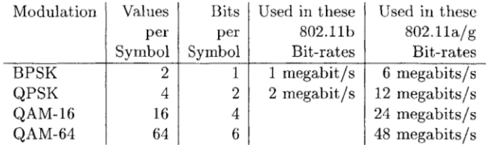
Figure 1-1: A summary of a few basic modulations used by 802.11.

1.1

Theoretical Considerations

This section presents a simple theoretical framework to explain why allowing links to choose from multiple modulations can increase link throughput when link qualities vary by a large amount. It ignores some practical considerations, such as noise other than additive Gaussian white noise, in order to be able to present the basic factors in modulation performance.

Each bit-rate uses a particular modulation to transform a data stream into a sequence of symbols which are encoded by changes in the amplitude, phase, or frequency of an analog signal. Assuming that the symbol rate is held constant, the amount of information each modulation can transmit over time is determined by the number of possible distinct values for each symbol. The set of distinct possible symbol values is called a constellation.

Figure 1-1 shows a summary of a few modulations that 802.11 uses to encode data. These modulations use x distinct values in a constellation to encode log2(x) bits. The minimum distance between any two values in a constellation determines the least amount of noise that is needed to generate a bit-error; denser constellations require a higher signal-to-noise ratio (S/N) to ensure they can decode every symbol correctly.

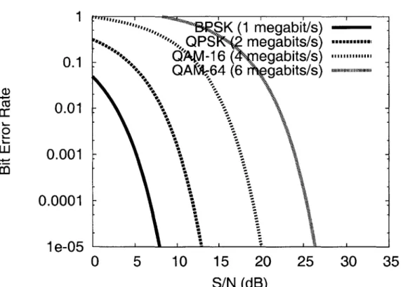
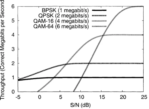
The amount of information received over a link is a function of the number of bits the receiver can decode correctly. Figure 1-2 plots the theoretical bit error rate (BER) against signal-to-noise ratio for several modulations, assuming a channel with only additive Gaussian white noise (AGWN), based on equations from [7]. Throughput over a link, in correct bits received per second, is the product of the symbol rate, bits per symbol, and the probability that a bit is received correctly (1 - BER). Figure 1-3 shows throughput versus

S/N for each modulation for a symbol rate of 1 mega-symbol per second.

through-1

,,,,,K (1

megabit/s)

P,

QP Si

megabits/s)

0.165V

QA 64 (6 rhogabits/s)

a)

0.01

0.001

0.0001

1e-05

0

5

10

15

20

25

30

35

S/N

(dB)

Figure 1-2: Theoretical bit error rate (BER) versus signal-to-noise ratio for several modu-lation schemes assuming AGWN. The y axis is a log scale. Higher bit-rates require larger

o

6

6

BPSK (1 megabit/s)

(n

QPSK (2 megabits/s)

L

5

QAM-16 (4 megabits/s)

-

C-Q-

_{QAM-64 (6 megabits/s)}

a)

-:.

3

-0

a)

2

0

0

-5

0

5

10

15

20

25

S/N

(dB)

Figure 1-3: Theoretical throughput in correct bits per second versus S/N for several mod-ulations, assuming AGWN and a symbol rate of 1 mega-symbol per second.

put. If a link's S/N were always 10 dB, then only QAM-16 would be required. However, if the link's S/N changed to 20, then the best throughput would be obtained by switching the modulation to QAM-64. Each modulation has a S/N for which it is most efficient; the modulation doesn't take advantage of higher S/N values, and the modulation's BER increases rapidly for lower S/N values. Thus, if a system must cope with a range of S/N values, it must also be able to switch between multiple modulations.

For S/N values up to 22 dB in Figure 1-3, the highest throughput modulation always experiences bit-errors. If real links behaved like Figure 1-3, bit-rate selection algorithms would need to be willing to tolerate loss in order to use the bit-rate that provided maximum throughput; they could not assume that links either worked perfectly or not at all.

802.11 groups bits into packets for lots of reasons, mostly to share the physical medium

among multiple senders. Receivers use checksums in each packet to detect bit-errors and discard packets with any bit-errors. The resulting throughput in bits per second for n-bit

0 CD CO

CZ

o

F-6

5

4

3

2

1

0

BPSK (1 regabit/s)

-QPSK (2 megabit/s)

QAM-16 (4 megabits/s)

QAM-64 (6

megabits/s)

F

5

10

15

20

25

30

S/N (dB)

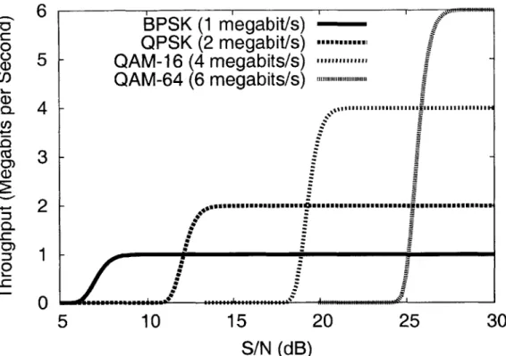
Figure 1-4: Theoretical throughput in megabits per second using packets versus signal-to-noise ratio for several modulations, assuming AGWN and a symbol rate of 1 mega-symbol per second.

packets can be estimated using the following equation:

throughput = (1 - BER)" * bitrate

This equation assumes the transmitter sends packets back-to-back, the receiver knows the location of each packet boundary, the receiver can determine the integrity of the data with no overhead, there is no error correction, and the symbol rate is 1 mega-symbol per second.

Packets change the throughput versus S/N graph dramatically; Figure 1-4 shows through-put in megabits per second versus S/N for 1500-byte packets after accounting for packet losses caused by bit-errors. The range where each modulation delivers non-zero throughput but suffers from loss is much smaller in Figure 1-4 than in Figure 1-3. For most S/N values in the range from 5 to 30 dB, the best bit-rate delivers packets without loss.

Bit-rate selection is easier for links that behave as in Figure 1-4 than as in Figure 1-3; the sender can start on the highest bit-rate and switch to another bit-rate whenever the

current bit-rate begins to experience packet loss. Occasionally the sender can try to send a packet at a higher bit-rate and change the bit-rate if this packet succeeds. Designing a well-performing scheme for Figure 1-4 is simpler than for Figure 1-3 because the regions where each bit-rate has intermediate delivery probabilities are smaller.

1.2

Practical Considerations

The previous section may give the impression that the performance of a particular bit-rate can be predicted using the signal-to-noise ratio of a link; earlier work [13, 6] has shown that link performance is often not well predicted by S/N in environments with reflective obstacles. In these environments, multi-path interference causes poor performance regardless of signal-to-noise ratios [3, 5]. These complications make the intermediate loss regions in Figure 1-4 much larger on real links and more like those in Figure 1-3. As a result, a key challenge in bit-rate selection is predicting which bit-rate will provide the most throughput.

Chapter 2

802.11 Background

This chapter describes the features of 802.11 that are relevant to this thesis. The IEEE

802.11 standards cover both the Physical Layer and the Medium Access Control (MAC)

layer.

2.1

Physical Layer

For the purposes of this thesis, the most important parts of the physical layer are the modulation techniques and channel coding. The original 802.11 standard [4] specified Direct

Sequence Spread Spectrum (DSSS) radios that operate at 1 megabit in the 2.4 gigahertz frequency range. 802.1lb added additional higher bit-rates, and 802.11g added bit-rates that use Orthogonal Frequency Division Multiplexing (OFDM). 802.11a allows use of frequencies at 5.8 gigahertz using only the OFDM bit-rates.

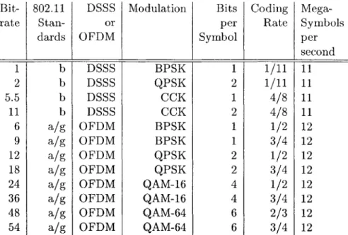
Figure 2-1 shows a summary of the modulations and channel coding for the bit-rates used in 802.11. Each bit-rate uses some form of forward error correction with a coding rate expressed by k/n, where n coded bits are transmitted for every k bits of data. The bit-rate is found by multiplying the coding rate, bits per symbol, and the number of sym-bols per second. DSSS bit-rates send one symbol at a time and OFDM bit-rates send 48 symbols in parallel; as a result, 5.5 megabits has a lower bit-rate than 6 megabits even though 6 megabits sends fewer bits per symbol, has a longer symbol length, and sends more redundancy for each bit.

The particular modulation and coding techniques that rates use are relevant to bit-rate selection because the techniques use different approaches to increase the capacity of

Bit- 802.11 DSSS Modulation Bits Coding Mega-rate Stan- or per Rate Symbols

dards OFDM Symbol per

second 1 b DSSS BPSK 1 1/11 11 2 b DSSS QPSK 2 1/11 11 5.5 b DSSS CCK 1 4/8 11 11 b DSSS CCK 2 4/8 11 6 a/g OFDM BPSK 1 1/2 12 9 a/g OFDM BPSK 1 3/4 12 12 a/g OFDM QPSK 2 1/2 12 18 a/g OFDM QPSK 2 3/4 12

24 a/g OFDM QAM-16 4 1/2 12

36 a/g OFDM QAM-16 4 3/4 12

48 a/g OFDM QAM-64 6 2/3 12

54 a/g OFDM QAM-64 6 3/4 12

Figure 2-1: A summary of the 802.11 bit-rates. Each bit-rate uses a specific combination of modulation and channel coding. OFDM bit-rates send 48 symbols in parallel.

a channel. In the presence of fading, multi-path interference, or other interference that is not additive white Gaussian noise, predicting the combinations of modulation and channel coding that will be most effective at masking bit errors is difficult.

All 802.11 packets contain a small preamble before the data payload which is sent at

a low bit-rate. The preamble contains the length of the packet, the bit-rate for the data payload, and some parity information calculated over the contents of the preamble. The preamble is sent at 1 megabit in 802.1lb and 6 megabits in 802.11g and 802.1la. This results in the unicast packet overhead being different for 802.11b and 802.11g bit-rates; a perfect link can send approximately 710 1500-byte unicast packets per second at 12 megabits (an

802.1lg bit-rate) and 535 packets per second at 1 megabit (an 802.1lb bit-rate). This means

that 12 megabits can sustain nearly 20% loss before a lossless 11 megabits provides better throughput, even though the bit-rate is less than 10% different.

2.2

Medium-Access Control (MAC) Layer

For the purposes of this thesis, the most important properties of the 802.11 MAC layer are the medium access mechanisms and the unicast retry policy.

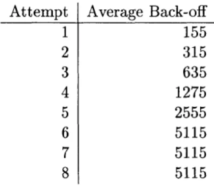
with collision avoidance (CSMA/CA). In CSMA/CA, nodes compare the energy present on the channel to a threshold in order to determine if the medium is busy. They also listen for any packet being sent on the network, and if they decode the physical header of the packet, they will mark the medium as busy for the duration of the transmission. Each node uses a back-off window to track how long it should defer sending packets after the medium has become idle. When a node wants to transmit a packet, it waits until the medium is idle for at least a Distributed Inter-Frame Gap (DIFS) and then picks a random time within its back-off window and waits until this time expires. If the medium has been idle during the entire back-off period, it sends the packet and resets the back-off window to the minimum value. Otherwise, it doubles the back-off window, waits until the medium is idle for at least a Distributed Inter-Frame Gap (DIFS) period of time, and begins the back-off period again. To mask losses from higher network layers when transmitting unicast packets, 802.11 uses link-level retransmissions. After each data packet is received, the recipient sends an acknowledgment to the transmitter indicating that the packet was received intact. The transmitter may resend the packet if no acknowledgment was received after doubling the back-off window and waiting another back-off period. Figure 2-2 shows the length of the average back-off period after a certain number of retries, assuming that the back-off window is at the minimum value on the first attempt and the medium is idle the entire time. If the back-off window is longer or if the medium is busy sometime during the transmission, these values will be higher. This is important for bit-rate selection because the back-off penalty may exceed the transmission time of a packet after a few retries, and backoff must be accounted for when estimating the transmission time of a packet.

1 155 2 315 3 635 4 1275 5 2555 6 5115 7 5115 8 5115

Figure 2-2: The average back-off period, in microseconds, for up to 8 attempts of a 802.11b unicast packet. For comparison, sending a 1500 byte broadcast packet at 11 megabits takes

1873 microseconds.

Chapter 3

Indoor Network Measurements

This chapter presents measurements taken on a 45-node indoor wireless test-bed, and makes the following observations related to bit-rate selection. There are a wide range of link qualities; often the bit-rate with the highest throughput suffers from a significant amount

of loss, but rarely more than 50%. The optimal bit-rate of a link does not change much over

intervals on the scale of seconds, allowing bit-rate selection algorithms to choose bit-rates based on measurements over a few seconds. Signal-to-noise ratio has little predictive value for loss rate or which bit-rate will provide the highest throughput.

3.1

Experimental Methodology

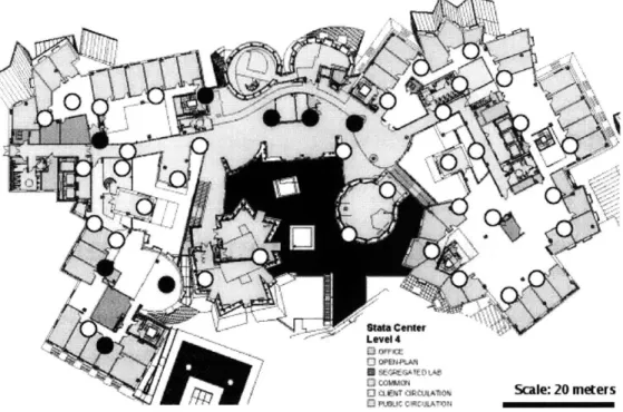
The data in this chapter are the result of measurements taken on a 45 node wireless test-bed. Each node is a small wireless router that runs Linux and has an Atheros 5212 PCI 802.11a/b/g card. These nodes are placed on the 4th and 5th floors of an office building. Figure 3-1 shows their positions. Most of the nodes were placed in cable trays that run along walls about 9 feet above the floor. Others were placed on the floor or around desks.

The cards are configured to send at a fixed power level. The Request-to-Send, Clear-to-Send (RTS/CTS) protocol is turned off. The cards operate in a "pseudo-IBSS" mode in which they send no management messages. Each data packet in the following measurements consists of 24 bytes of 802.11 header, 1500 bytes of data payload, and 4 bytes of a frame

check sequence.

802.11 link level acknowledgments are used for each unicast packet. 802.11 does not

Figure 3-1: A map of the 4th and 5th floor indoor network. Node locations are marked by a box and a node identifier. Nodes filled in with black are located on the 5th floor.

To minimize interference, the nodes operated on channel 16 when using 802.llb and 802.11g. Access points present in the building operated on channels below 11. 802.lla experiments were run on channel 149, and no 802.lla access points were known to be present. No other traffic was observed on the channel for a 10 second period before each of the experiments.

3.2

Bit-rate, Throughput, and Packet Loss

This section presents measurements from a link level broadcast experiment. For the duration of the experiment, each node sends broadcast packets as fast as it can for 90 seconds at each bit-rate in turn. Only one sender sends at a time. The packets are 1500 bytes long including the 802.11 header. The other nodes record which of the packets they receive.

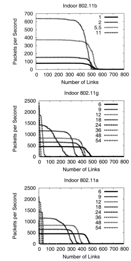
Figure 3-2 shows the link distribution of delivery rates for different bit-rates with 1500-byte broadcast packets at 802.lla, 802.llb, and 802.llg bit-rates. The data for each bit-rate is sorted separately, so the delivery rates for any particular x value are not typically from the same pair of nodes. These graphs show that intermediate delivery rates exist for many bit-rates. One example is 24 megabits in 802.llg; most of the 24 megabit links are lossy.

This can be a problem for bit-rate selection algorithms that assume bit-rates either work well or not at all.

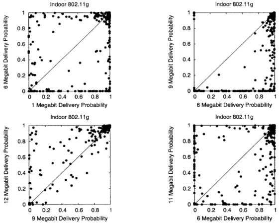
Figure 3-3 contains several graphs plotting the delivery probabilities of two bit-rates across the same set of links. These graphs demonstrate that if two bit-rates use similar channel coding and modulation techniques, the higher bit-rate will usually work only if the lower bit-rate works well. For instance, most links only work at 9 megabits if they have a delivery probability greater than 80% at 6 megabits. This can be explained because they both use BPSK modulation, but 6 megabits uses a coding rate of 1/2 and 9 megabits uses 3/4. One would expect these bit-rates to react similarly to interference, multi-path reflections, and noise in the environment, and that 6 megabits would be more robust because it sends more redundancy for every bit.

One example comparing different modulation techniques is the graph for 1 and 6 megabits. These modulations are very different; they both use BPSK, but 1 megabit uses DSSS and

6 megabits uses OFDM. There are many links that can operate at 1 megabit but not 6 and

vice-versa. Similar effects occur at 9 and 12 megabits (9 uses BPSK with a coding rate of 3/4 while 12 uses QPSK with a coding rate of 1/2) as well as 6 and 11 megabits (6 uses

OFDM and BPSK while 11 uses DSSS and CCK).

One conclusion from Figure 3-3 is that bit-rate selection algorithms cannot assume that a lower bit-rate will always have a have a better delivery probability than a higher one.

3.3

Adaptation Interval

The time scale at which link conditions change dictates how quickly bit-rate selection algo-rithms must adapt. If a higher bit-rate alternated between intervals of delivery and total loss while a lower bit-rate delivered all the packets, a bit-rate selection algorithm that reacted to link changes quickly enough could take advantage of the higher bit-rate's intervals of de-livery. If packet delivery probabilities were relatively constant for intervals longer than ten seconds, then bit-rate selection algorithms could choose the bit-rate based on measurements over a few seconds and still achieve high throughput.

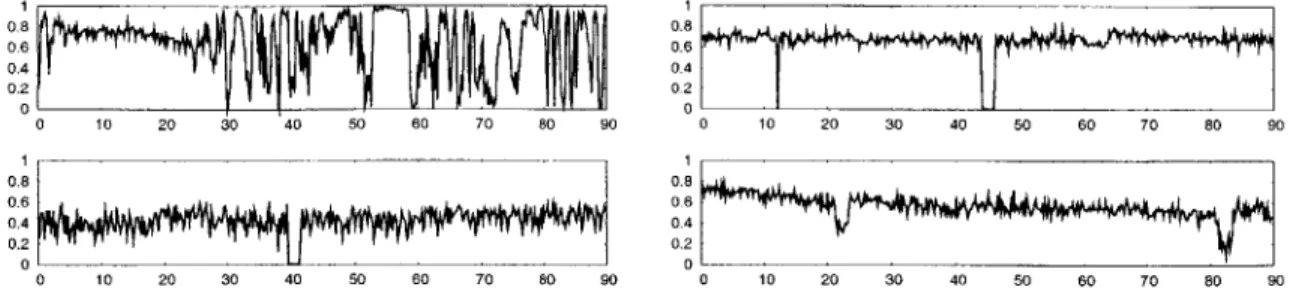
Figure 3-4 shows delivery probability over time for four links transmitting 1500-byte broadcast packets at 11 and 6 megabits and shows how bit-rate performance changes over time. The lines indicate averages over successive 200-millisecond intervals. The four links

- ----

~--~-Indoor 802.11 b

600

500

400

300

200

100

0

2500

2000

1500

1000

500

0

2500

2000

1500

1000

500

0

-5.5

"

0

100 200 300 400 500 600 700 800

Number of Links

Indoor 802.11 g

0

100 200 300 400 500 600 700 800

Number of Links

Indoor 802.11 a

0 100 200 300 400 500 600 700 800

Number of Links

Figure 3-2: The distribution of link throughputs for 1500-byte broadcast packets at different bit-rates. Each point corresponds to one sender/receiver pair at a particular bit-rate. Points were restricted to pairs that managed to deliver at least one packet during the experiment. Each point on the x axis represents a link and the lines are sorted independently.

_0 0 CD) U) a) CL, U) 0z CL

_0

C)

Co

U)

6

-12

18

24

-

54.

36

...

-6

9

...

12

...

18

---24

~

54

i...---"

Indoor 802.11 g Doi *. *.. *s 0 * 0 * 0, Aw 0 0.2 0.4 0.6 0.8 1

1 Megabit Delivery Probability

Indoor 802.11 g - ₀ ?00 00- *0. -0 * 0* CU -0 0 CU 0) (D) a. 0) (D 0 0.2 0.4 0.6 0.8 1

9 Megabit Delivery Probability

Figure 3-3: Comparison plots for individual shows the delivery probability of one link at similar modulation and coding techniques will

0.8 0.6 0.4 0.2 0 0.8 0.6 0.4 0.2 01 Indoor 802.11 g ** 0 e * , 0 0.2 0.4 0.6 0.8 1

6 Megabit Delivery Probability

Indoor 802.11 g 0 *.* o 00 0 O . *, **,* P 0 0* 0 0.2 0.4 0.6 0.8 1

6 Megabit Delivery Probability

bit-rates. Each point in these scatter plots two different bit-rates. Bit-rates that use [have points all to one side of x = y.

Cz -0 2~ I0 CD 0.8 0.6 0.4 0.2 A Ca M0 2 a. a) Cu 0) 0.8 0.6, 0.4 0.2 01 1

0.8 0.6 0 00 10 20 30 '40 50 60 70 80 90 1 1 0.8 0.8

L

J

Figure 3-4: Delivery probability over time (in seconds) for several links with approximately

50% average loss rate. The top two graphs show 11 megabit 802.11b links while the bottom

two show 6 megabit 802.llg links. Each point is an average over 200 milliseconds. The top left graph shows one of the network's most bursty links and the rest show links of average burstyness.

are chosen from among the set of links with delivery probabilities near 50%; the top left graph shows the link from the set of links with the highest short-term variation in delivery probability, and the remaining graphs show links with short-term variation typical of links in the network.

To understand how the adaptation interval affects link throughput, each node took a turn sending 1500-byte packets interleaved at 6, 9, 12, 18, and 24 megabits repeatedly for 90 seconds over an 802.1 la channel on the indoor network. For various values of t, data for each link is divided into t-millisecond intervals. The throughput estimate for each bit-rate during an interval is calculated using its delivery probability, and the throughput for an interval is the highest throughput estimate of all the bit-rates. The estimated total throughput for each value of t is the average of the throughput for all the t-millisecond intervals.

Figure 3-5 shows the results for the adaptation interval experiment over intervals from

100 milliseconds to 50 seconds. For each interval, this graph shows the average throughput

as well as the estimated total throughput for the 90th percentile link and the 10th percentile link. The x-axis indicates the decision time t and is a log scale. A bit-rate selection algorithm that selects the the bit-rate every 32 seconds will perform, on average, half as well as an algorithm that selects the optimal rate at 16 second intervals. Figure 3-5 demonstrates that there is very little performance reward for selecting the bit-rate more often than every 10 seconds. 0.8 0.6 0.4 0.2 0 0 10 20 30 40 50 60 70 80 90

0 2500 U) 2000 CL 1500 CO) 1000 _c 500 0

~wiI

Adaptation Interval (Milliseconds)

Figure 3-5: Average link throughput versus adaptation interval. This graph shows the average throughput over all non-zero links for different bit-rate adaptation intervals. Crosses mark the throughput of the average link, and error bars show the 90th and 10th percentile link throughput. This graph shows that there is little difference between selecting the bit-rate every 200 milliseconds instead of every 5 seconds, but that using intervals much greater than 10 seconds decreases throughput.

3.4

Signal-to-noise Ratio and Loss Rate

A close correlation between signal-to-noise ratio and the delivery probability at each bit-rate

would make bit-rate selection relatively straightforward; a receiver could send measurements of the the signal-to-noise ratio (S/N) of a link to the sender, and the sender could use these

measurements to choose the bit-rate on the link.

Figure 3-6 shows a scatter plot of S/N versus delivery probability. Each point indicates the average delivery ratio and the average S/N for all the packets received for each link. This data was obtained during a single broadcast experiment on a 38-node outdoor wireless network, where each node sequentially sends 1500-byte 802.11 broadcast packets as fast as it can while the rest of the nodes passively listen. More results from these experiments are detailed in [2]. The receiver records the signal and noise values the Prism II 802.11 card reports for each packet.

For almost all bit-rates, a S/N greater than 30dB indicates that a bit-rate will be lossless. Picking a threshold to determine if a bit-rate "works" is difficult; for example, delivery probabilities for 1 megabit packets with a S/N of 10dB range from 2% to 100%. Any S/N threshold will either omit links that perform well or will include links that do not. It is possible that variations in receive sensitivity across the nodes could be responsible

1-0.8 0.6 0.4 0.2 -0 0 5 10 15 20 25 30 35 40 45 5' S/N (dB) . yl !P ..-- -- ' *Ire

.-Ae*

Figure 3-6: Delivery probability at 1, 2, 5.5, and 11 megabits versus the average S/N. Each data point represents an individual sender-receiver pair.

0.8 * -0.6 0.4 0.2 0 *' -5 0 5 10 15 20 25 30 35 S/N (dB) 0.8 -. g 0.6 -.-0.4 -* 0.2 - . 0 "" -5 0 5 10 15 20 25 30 35 S/N (dB) CU 2 a-a) 2 1 0.8a 0.6-0.4 0.2 n 0 ,' -5 0 5 10 15 20 25 30 35 S/N (dB) 1 0.8 0.6 0.4 0.2 . -50 -5 0 5 10 15 20 25 30 35 S/N (dB)

Figure 3-7: A scatter plot of average S/N vs average delivery probability at 1 megabit. Each graph corresponds to a different receiver. Each point shape corresponds to a different sender. There is a point per one-second interval per sender.

.; * 2.64 -. N e. . . . -0 5 1-0 15 2-0 25 3-0 35 4-0 45 5-0 S/N (dB) 1 0.8 0.6 0.4 0.2 0 Ca .0 0 a a) 0

600- 600- 600-0 0 0 0 Q

~400-

Bit-rate Bit-rate Bit-rate

Steep

Gradual

Lossy

Figure 3-8: Three examples of possible link behavior. In each example, the gray bars are the maximum throughput for each 802.11b rate. The black bars are the throughput that the link is able to achieve at that bit-rate. The graph on the far left shows a steep drop-off; the bit-rates work perfectly until they do not work at all. The middle graph shows a gradual falloff in throughput after 5.5 megabits. The graph on the right shows a link where all bit-rates are lossy, but 11 megabits still provides the highest throughput.

for the spread of S/N values in Figure 3-6, but individual nodes might have a stronger relationship between S/N and delivery probability. Figure 3-7 shows per-receiver versions of the 1 megabit plot from Figure 3-6. These plots show a stronger correlation between S/N and delivery probability, although there are several points in these graphs that suggest signal-to-noise ratio does not accurately predict delivery probability; trying to pick a threshold to determine whether a link operates at a particular bit-rate will result in some links that do not work (because the threshold was too low for some links) or links that offer sub-optimal throughput (because the threshold is too high for some links).

3.5

Link Classification and Bit-rate Throughput

The relationship between bit-rate and throughput on individual links dictates which assump-tions algorithms can rely on to simplify bit-rate selection without sacrificing throughput. Figure 3-8 shows three examples of the throughput that the 802.11b bit-rates achieve over individual links. If all links looked like the steep example in figure 3-8, where each increas-ing bit-rate worked perfectly until all bit-rates ceased to work altogether, then designincreas-ing an algorithm to find the bit-rate with the highest throughput would be simple; you could pick the highest bit-rate that delivered any packets. However, such an algorithm might prove disastrous if used in links that behave like the gradual example in Figure 3-8, where the throughput falls off more slowly. In this case, the algorithm for the steep model would

Network Total Steep Gradual Lossy Other Indoor 802.11a 100 26 41 22 0

Indoor 802.11g 108 16 86 21 0

Indoor 802.11b 168 98 144 24 0

Outdoor 802.11b 36 5 23 13 0

Figure 3-9: A taxonomy of links. The relationship between bit-rate and throughput is classified for each non-zero unicast link according to the types in Figure 3-8.

choose 11 megabits which delivers only a third of the throughput of 5.5 megabits. Finally, if links behaved like the lossy example, bit-rate selection algorithms would have to be willing to choose bit-rates with high loss rates and could not assume that higher bit-rates have low throughput if low bit-rates suffer from significant loss.

To understand how many of each kind of link exists, the unicast performance of each bit-rate was measured for a number of links. Links were chosen from non-zero pairs in the broadcast experiments discussed earlier in this chapter.

For purposes of classification, a link matched the steep model if the all bit-rates achieved at least 90% of their possible throughput or less than 10% of the maximum throughput. A

gradual link is one whose best performing bit-rate is the highest one that has more than

50% delivery rate. A lossy link is defined as a link where the best bit-rate has lower than 50% delivery rate. A link that fit none of the descriptions is classified as other.

Figure 3.5 shows the results of the link classification. Most of the links, regardless of network type, matched the gradual model. Because so many links fit the gradual model, an algorithm that finds the highest bit-rate operating with less than 50% loss will usually find the optimal bit-rate. A higher percentage of links match the lossy model on the outdoor network than on the indoor network; almost 40% of the outdoor 802.11b links classified as

lossy. As a result, bit-rate selection algorithms that perform well indoors may not perform

Chapter 4

Related Work

This chapter discusses previous research related to bit-rate selection algorithms.

4.1

Auto Rate Fallback (ARF) and Adaptive ARF (AARF)

The first documented bit-rate selection algorithm, Auto Rate Fallback (ARF) [9], was devel-oped for WaveLAN-II 802.11 cards. These cards were one of the earliest multi-rate 802.11 cards and could send at 1 and 2 megabits. ARF aims to adapt to changing conditions and take advantage of higher bit-rates when opportunities appear. ARF was also designed to work on future WaveLAN cards with more than 2 bit-rates.

For a particular link, ARF keeps track of the current bit-rate as well as the number of successive transmissions without any retransmissions. Most 802.11 wireless cards offer feedback about packet transmission after the transmission has either been acknowledged or exceeded the number of retries without an acknowledgment.

When the ARF algorithm starts for a new destination, it selects the initial bit-rate to be the highest possible bit-rate. Given the number of retries that a transmission used and whether or not it was successfully acknowledged, ARF adjusts the bit-rate for the destination based on the following criteria:

" Move to the next lowest bit-rate if the packet was never acknowledged.

" Move to the next highest bit-rate if 10 successive transmissions have occurred without

any retransmissions.

The main advantages of ARF are that it is easy to implement and it has very little state.

If unicast packet loss is relatively inexpensive, the ARF algorithm will work particularly well

on links similar to the steep example in Figure 3-8. For these links, bit-rates either work well or not at all, there are no lossy bit-rates, and lower bit-rates always have better delivery probabilities than higher bit-rates. ARF works well in these situations because it will increase the bit-rate to the highest one that works because all the bit-rates that can deliver packets do so without loss; ARF will try to step up occasionally, but it will immediately step down when this occurs. The ARF algorithm also performs well in situations where link conditions change on the order of tens of packets. It reacts particularly well to link

degradation; within a few packets it can step down to the lowest bit-rate.

ARF performs poorly in situations where links experience loss as shown in the lossy or

gradual graphs of Figure 3-8. In these situations, ARF may increase the bit-rate past the

highest throughput one to another which requires many retries for each packet. Throughput of this bit-rate may be very low, but ARF does not step down until a bit-rate experiences packet failure. As a result, ARF may spend a significant amount of time transmitting packets at a higher bit-rate that does not work well. Alternatively, ARF may decrease the bit-rate because of packet failures but it may not step up again to a better performing bit-rate if lower bit-rates are lossy.

Adaptive Auto Rate Fallback (AARF) [11] is an extension of ARF where the step-up parameter is doubled every time the algorithm tries to increase the bit-rate and the subsequent packet fails. This can increase throughput dramatically if packet failures take up a large amount of transmission time. This occurs with the higher bit-rates of 802.11g and 802.11a since the back-off penalty is so high. A 1500 byte unicast packet with no retries takes 560 microseconds at 36 megabits and 730 microseconds at 24 megabits. A unicast packet that is sent 5 times at 36 megabits, without being acknowledged, will take an average

of 11,510 microseconds. If ARF operates on a link where 24 megabits works but 36 megabits

does not at all, it will send packets at 24 megabits except every 10th packet will be sent at 36 megabits. Since every 10th packet will fail to be acknowledged, that one packet will take up more transmission time (11510 microseconds) than the other 9 packets combined

(6579 microseconds). AARF will instead wait exponentially longer before increasing the

bit-rate if no other packet failures occur, which allows it to avoid the throughput reduction resulting from trying high bit-rates that do not work.

4.2

Onoe

The 802.11 device driver for Atheros cards in Linux and FreeBSD [1] contains the only openly available bit-rate selection algorithm designed to work with 802.11b, 802.11g, and 802.11a devices. The Onoe algorithm is much less sensitive to individual packet failure than the ARF algorithm, and basically tries to find the highest bit-rate that has less than 50% loss rate.

For each individual destination, the Onoe algorithm keeps track of the current bit-rate for the link and the number of credits that bit-rate has accumulated. It only keeps track of these credits for the current bit-rate and increments the credit if it is performing with very little packet loss. Once a bit-rate has accumulated a threshold value of credits, Onoe will increase the bit-rate. If a few error conditions occur, the credits will be reset and the bit-rate will decrease.

When packets are first sent to a destination, Onoe sets the initial bit-rate to 24 megabits in 802.11g and 802.11a and 11 megabits in 802.11b. It also sets the number of credits for that bit-rate to 0. The Onoe algorithm performs the following operations periodically for every destination (the default period is one second):

" If no packets have succeeded, move to the next lowest bit-rate and return.

" If 10 or more packets have been sent and the average number of retries per packet

was greater than one, move to the next lowest bit-rate and return.

" If more than 10% of the packets needed a retry, decrement the number of credits (but

don't let it go below 0) and return.

" If less than 10% of the packets needed a retry, increment the number of credits.

" If the current bit-rate has 10 or more credits, increase the bit-rate and return.

" Continue at the current bit-rate.

The Onoe algorithm works particularly well in situations such as the gradual example in Figure 3-8. In this situation, the bit-rates work well until they start to fall off. Onoe is trying to find the highest bit-rate with less than a 50% loss rate, so it will step down from

802.11 b Delivery Probability versus Throughput 802.11 a Delivery Probability versus Throughput 1 . . 1 1 x+ 0.9 ++ x 0 U 0 0 5 .5 * - x . + x0, 7 + x 0 0.9 - + x 0 0 + x 0. + " 0 .0 +1XX S 05 +x 0 E. 0.5 6 + 0.25 + _{1 0.4} - +x0 + ₁₂ 2 x -0.3 +XX 18 +* 0.2 24 L 0. ' w ' 'c1 '0.5 + -3wo6 + +X AO > 0.1 ) 0 100 200 300 400 500 600 0 2004006008001000 200 400 600 800

Throughput (Packets per Second) Throughput (Packets per Second)

Figure 4-1: Simulated average delivery probability versus throughput for 802.11b and 802.11a bit-rates. The Onoe algorithm chooses the highest bit-rate that has less than

50% loss. The maximum throughput of the 802.11b bit-rate operating with 50% loss is

close to the maximum throughput of the next lowest bit-rate. The maximum throughput for the 802.11a bit-rates are not spaced as far apart.

Figure 4-1 shows the relationship between average delivery rate and throughput for the

802.11b and 802.Ila rates and helps explain why Onoe steps down to the next lowest

bit-rate when the current bit-bit-rate experiences more than 50% loss. The maximum throughputs for the 802.11b bit-rates are spaced apart at powers of two (78, 152, 372, and 637 packets per second at 1500 bytes). Since the throughput of the next lowest bit-rate in 802.11b is usually half the current bit-rate, the current bit-rate will generally perform better until it sees at least 50% loss, which is when Onoe will to step down to the next lowest bit-rate. Onoe might select low-throughput bit-rates in 802.11a because the 802.11a bit-rates are much closer together; Figure 4-1 shows that a 36 megabit link with 50% loss gets about half the throughput that a perfect 24 megabit achieves.

The Onoe algorithm is relatively conservative; once it decides a bit-rate will not work, it will not attempt to step up again until at least 10 seconds have gone by. The Onoe algorithm can also take time to stabilize. It will only step down one bit-rate during each period, so it can take a few seconds before the Onoe algorithm can send packets if it starts at a bit-rate that is too high for a given link.

4.3

Receiver Based Auto-Rate (RBAR)

Receiver Based Auto-Rate (RBAR) [8] chooses the bit-rate based on S/N measurements at the receiver. The basic intuition is that channel quality seen by the receiver is what determines whether a packet can be received. When a receiver gets an RTS packet, it calculates the highest bit-rate that would achieve a BER less than 10-5 based on the S/N of the RTS packet using functions in [8]. The receiver piggybacks the bit-rate on the CTS packet, and the sender uses that bit-rate to send the data packet. RBAR is designed to work well in mobile environments in which channel conditions may change on packet timescales. RBAR makes the assumption that the receiver can compute the best bit-rate for a data packet from the S/N of an RTS packet. This thesis presents data in Chapter 3 that suggests

S/N values have little predictive value in our networks.

4.4

Opportunistic Auto-Rate (OAR)

Opportunistic Auto-Rate (OAR) [12] takes advantages of higher bit-rates when rapid changes in channel quality take place. OAR nodes opportunistically send multiple back-to-back data packets whenever the channel quality is good; this allows OAR to increase channel through-put by allocating equal amounts of transmission time to senders.

The intuition behind OAR is that channel coherence times typically exceed multiple packet transmission times, and by taking advantage of high link qualities when they appear, channel throughput can be increased. OAR uses the RTS/CTS exchange for rate control purposes (like RBAR), but grants each sender the same amount of time in the CTS as the transmission time of a packet at the base rate. Other nodes that hear the CTS will not send during this time, and if the link is performing well, the sender can send multiple packets at a high bit-rate in the same time that one transmission would take at a lower bit-rate.

The evaluation of OAR uses RBAR as a bit-rate selection algorithm, and integration of other sender-based rate control algorithms is discussed. This thesis focuses on bit-rate selection on individual links, which has a direct impact on the performance of protocols like

Chapter 5

Design

This chapter presents the design of the SampleRate bit-rate selection algorithm. SampleR-ate maximizes throughput by sending packets at the bit-rSampleR-ate that has the smallest average packet transmission time as measured by recent samples. A key aspect of the design of SampleRate is the way it periodically sends packets at bit-rates other than the current bit-rate to estimate their average transmission time.

SampleRate must address the following challenges when trying to pick the optimal bit-rate:

" A bit-rate selection algorithm cannot conclude that higher bit-rates will perform

poorly just because lower bit-rates perform poorly (Section 3.5).

" The bit-rate that achieves the most throughput may suffer from a significant amount

of loss. Algorithms that only use bit-rates with high delivery probability may not find the bit-rate that achieves the highest throughput (Section 3.2).

" Link conditions may change. Failing to react to changes in link conditions could result

in needlessly low throughput (Section 3.3).

" A rate selection algorithm that constantly measured the throughput of every

bit-rate would likely achieve low throughput. If a link sends every 10th packet at a bit-bit-rate that requires 4 retries, it might get only half the throughput it is capable of. Bit rate selection algorithms must limit the bit-rates they choose to measure.

SampleRate sends data at the bit-rate that has the smallest predicted average packet transmission time, including time required to recover from losses. SampleRate predicts the

estimated packet transmission time by averaging the transmission times of previous packet transmissions at a particular bit-rate. SampleRate periodically sends packets at a bit-rate other than the current bit-rate to gather information about other bit-rates. SampleRate reduces the number of bit-rates it must sample by eliminating bit-rates that could never send at higher rates than the current bit-rate that is being used. SampleRate also stops probing at a bit-rate that experiences several successive failures. SampleRate calculates the average transmission time using packets sent during the last ten seconds so that SampleRate can adapt to changing link conditions.

5.1

Algorithm

When a link begins to send packets, SampleRate sends data at the highest possible bit-rate. SampleRate stops using a bit-rate if it experiences four successive failures, so when first sending packets over a link SampleRate will decrease the bit-rate until it finds a bit-rate that is capable of sending packets. Every tenth data packet, SampleRate picks a random bit-rate from the set of bit-rates that may do better than the current one and sends the packet using that bit-rate instead of the current one. A bit-rate is not eligible to be sampled if four recent successive packets at that bit-rate have been unacknowledged or if its lossless transmission time (without any retries) is greater than the average transmission time of the current bit-rate.

To calculate each bit-rate's average transmission time, SampleRate uses feedback from the wireless card to calculate how much time each packet transmission required. For each transmitted packet, 802.11 wireless cards indicate whether the packet was successfully ac-knowledged and how many times the card sent the packet. SampleRate calculates the transmission time for each packet using the packet length, bit-rate, and the number of re-tries (including 802.11 back-off). SampleRate calculates the average transmission time for a bit-rate by averaging the packet transmission times of previous packets sent at that bit-rate. To avoid using stale information, SampleRate only calculates the average transmission time over packets that were sent within the last averaging window. This averaging window is set

to ten seconds based on link measurements from Chapter 3 showing that the best bit-rate changes little over ten second periods.

1500-Bit- Tries Packets Succ. Total Avg Lossless Destination rate Ack'ed Fails TX TX TX Time Time Time 00:05:4e:46:97:28 11 16 0 4 250404 00 1873 00:05:4e:46:97:28 5.5 100 100 0 297600 2976 2976 00:05:4e:46:97:28 2 0 0 0 0 - 6834 00:05:4e:46:97:28 1 0 0 0 0 - 12995 00:0e:84:97:07:50 11 28 14 0 52654 3761 1873 00:Oe:84:97:07:50 5.5 50 46 0 148814 3235 2976 00:0e:84:97:07:50 2 0 0 0 0 - 6834 00:0e:84:97:07:50 1 0 0 0 0 - 12995

Figure 5-1: This figure shows a snapshot of the statistics that SampleRate tracks for two destinations. For the top destination, 11 megabits delivers no packets but 5.5 works per-fectly. For the bottom destination, 11 megabits always requires a single retry and 5.5 megabits needs a retry on 10% of the packets. In both examples, 1 and 2 megabits will not be sampled because their lossless transmit time is higher than the average transmit time of

5.5 megabits.

byte packets. Destination 00:05:4e:46:97:28 has the properties that 11 megabits delivers no packets and all packets sent at 5.5 megabits are acknowledged successfully without retries. The first few packets sent on this link at 11 megabits failed, and once the "Successive Fail-ures" column reached 4 SampleRate stopped sending packets at 11 megabits. SampleRate then proceeded to send 100 packets at 5.5 megabits. Packets were never sent at 1 or 2 megabits because their lossless transmission time is higher than the average transmission time for 5.5 megabits.

The destination 00:0e:84:97:07:50 in Figure 5-1 has the properties that packets sent at

11 megabits require a retry before being acknowledged, and packets sent at 5.5 megabits

require no retries 90% of the time and one retry otherwise. On this link, SampleRate starts at 11 megabits and then sends the 10th packet at 5.5 megabits. After the first 5.5 megabit packet required no retries, SampleRate determined that 5.5 megabits took less transmit time, on average, than 11 megabits and switched bit-rates. It still sent at 11 megabits once every 10 packets to see if performance has improved at that bit-rate. SampleRate does not try to send packets at 1 or 2 megabits because the lossless transmission time for those bit-rates is higher than the average transmission time for both 11 and 5.5 megabits.

5.2

Implementation

SampleRate is implemented in three functions: apply-rateO, which assigns a bit-rate to a packet, process-f eedbacko, which updates the link statistics based on the number of retries a packet used and whether the packet was successfully acknowledged, and remove-stale-results(, which removes results from the transmission results queue that were obtained longer than

10 seconds ago. remove-stale-results() and apply-rate() are called, in that order,

immedi-ately before packet transmission and process-f eedback() is called immediimmedi-ately after packet transmission.

SampleRate maintains data structures that keep track of the total transmission time, the number of successive failures, and the number of successful transmits for each bit-rate and destination as well as the total number of packets sent across each link. It also keeps a queue of transmission results (transmission time, status, destination and bit-rate) so it can adjust the average transmission time for each bit-rate and destination when transmission results become stale.

apply-rate() performs the following operations:

" If no packets have been successfully acknowledged, return the highest bit-rate that

has not had 4 successive failures.

" Increment the number of packets sent over the link.

" If the number of packets sent over the link is a multiple of ten, select a random bit-rate

from the bit-rates that have not failed four successive times and that have a minimum packet transmission time lower than the current bit-rate's average transmission time.

" Otherwise, send the packet at the bit-rate that has the lowest average transmission

time.

When process-feedback() runs, it updates information that tracks the number of

sam-ples and recalculates the average transmission time for the bit-rate and destination. process-f eedback() performs the following operations:

* Calculate the transmission time for the packet based on the bit-rate and number of retries using Equation 5.1 below.

" Look up the destination and add the transmission time to the total transmission times for the bit-rate.

" If the packet succeeded, increment the number of successful packets sent at that bit-rate.

" If the packet failed, increment the number of successive failures for the bit-rate.

Oth-erwise reset it.

" Re-calculate the average transmission time for the bit-rate based on the sum of

trans-mission times and the number of successful packets sent at that bit-rate.

" Set the current-bit rate for the destination to the one with the minimum average

transmission time.

" Append the current time, packet status, transmission time, and bit-rate to the list of

transmission results.

SampleRate's remove-stale-results() function removes results from the transmission results queue that were obtained longer than ten seconds ago. For each stale transmission result, it does the following:

" Remove the transmission time from the total transmission times at that bit-rate to

that destination.

" If the packet succeeded, decrement the number of successful packets at that bit-rate

to that destination.

After remove-stale-results() performs these operations for each stale sample, it

re-calculates the minimum average transmission times for each bit-rate and destination. remove-stale-results() then sets the current bit-rate for each destination to the one with the smallest average

trans-mission time.

To calculate the transmission time of a n-byte unicast packet given the bit-rate b and number of retries r, SampleRate uses the following equation based on the 802.11 unicast retransmission mechanism detailed in Section 2.2:

where difs is 50 microseconds in 802.11b and 28 microseconds in 802.11a/g, sifs is 10 microseconds for 802.1lb and 9 for 802.1la/g, and ack is 304 microseconds using 1 megabit acknowledgments for 802.11b and 200 microseconds for 6 megabit acknowledgments. header is 192 microseconds for 1 megabit 802.11b packets, 96 for other 802.11b bit-rates, and 20 for 802.1la/g bit-rates. backof

f(r)

SampleRate has been implemented as part of the Click Modular Router [10]. The Click toolkit can run in both user-space and the kernel. SampleRate requires a modified version of the Madwifi device driver for Atheros based 802.11a/g/b cards. The primary modification added a fake packet header to packets so that applications like Click could communicate with the device driver and set the bit-rate on a per packet basis.

Chapter 6

Evaluation

This chapter evaluates the ARF, AARF, Onoe, and SampleRate bit-rate selection algo-rithms and compares their performance on a 45-node indoor test-bed and a 38-node outdoor test-bed. The main conclusions are that: ARF and AARF perform poorly on the test-beds; Onoe performs well on all but very lossy links; and SampleRate always performs very close to the best static bit-rate.

The ARF algorithm performs poorly in the test-bed because it spends too much time sending packets at bit-rates other than the one with the most throughput. The Onoe al-gorithm performs well in all cases except for very lossy links because it picks the highest

bit-rate with less than 50% loss, which is often the bit-rate with the best throughput. Sam-pleRate performs well on all links and performs better than the other algorithms on links where all bit-rates have intermediate delivery probabilities. Finally, lost 802.11 acknowl-edgments are common and often result in higher bit-rates being unusable for unicast traffic in spite of high data delivery probability.

6.1

Methodology

The experimental results presented in this section were obtained on the indoor testbed described in Chapter 3 and on an outdoor mesh network with 38 nodes. Tests on both net-works were run over links randomly selected from the set of links with non-zero broadcast throughput in the link-level broadcast experiments presented in Chapter 3. Each bit-rate selection algorithm ran for 30 seconds over each link. During these 30 seconds, the trans-mitter sent 1500-byte unicast packets as fast as it could.