ASSESSMENT OF THE USE OF PROMPT GAMMA EMISSION FOR PROTON THERAPY RANGE VERIFICATION
BY
JOHN R STYCZYNSKI
SUBMITTED TO THE DEPARTMENT OF NUCLEAR SCIENCE AND ENGINEERING IN PARTIAL FULFILLMENT OF THE REQUIREMENTS FOR THE DEGREES OF
MASTER OF SCIENCE IN NUCLEAR SCIENCE AND ENGINEERING AND
BACHELOR OF SCIENCE IN NUCLEAR SCIENCE AND ENGINEERING AT THE
MASSACHUSETTS INSTITUTE OF TECHNOLOGY
JUNE 2009
©2009 Massachusetts Institute of Technology All rights reserved
ARCHIVES
MAASSACHUSETTS H NSUTITUTEI OF TECOLO YAUG 19
2009
Ul RARF
Signature of Author
John R. Styczynski
Department of Nuclear Science and Engineering
15 May 2009
Certified by/7
Senior Resc
Scientist in Nuclear Science and Engineering, MIT
Richard C. Lanza
i h -
.1
Thesis Supervisor
Certified by
Harald Paganetti
Associate Professor of Radiation Oncology, Massachusetts General Hospital
A
Thesis Reader
Certified by
Accepted by
Jacquelyn C. Yanch
Prfeor in Nuclea
ience and Engineering, MIT
Thesis Reader
?
I
/Jacquelyn
C. Yanch
Professor in Nuclear Science and Engineering
Chair, Department Committee on Graduate Students
IASSESSMENT OF THE USE OF PROMPT GAMMA EMISSION FOR PROTON
THERAPY RANGE VERIFICATION
Submitted to the Department of Nuclear Science and Engineering on 15 May 2009 in Partial
Fulfillment of the Requirements for the Degrees of Master of Science in Nuclear Science and
Engineering and Bachelor of Science in Nuclear Science and EngineeringABSTRACT
PURPOSE: Prompt gamma rays emitted from proton-nucleus interactions in tissue present a promising non-invasive, in situ means of monitoring proton beam based radiotherapy. This study investigates the fluence and energy distribution of prompt gamma rays emitted during proton irradiation of phantoms. This information was used to develop a correlation between the measured and calculated gamma emission and the proton beam range, which would allow treatments to more effectively exploit the sharp distal falloff in the dose distributions of protons. METHOD & MATERIALS: A model of a cylindrical Lucite phantom with a monoenergetic proton beam and an annular array of ideal photon tallies arranged orthogonal to the beam was developed using the Monte Carlo code MCNPX 2.6.0. Heterogeneous geometries were studied by inserting metal implants into the Lucite phantom, and simulating a phantom composed of bone and lung equivalent materials and polymethyl methacrylate.
RESULTS: Experimental and computational results indicated a correlation between gamma emission and the proton depth-dose profile. Several peaks were evident in the calculated energy spectrum and the 4.44 MeV emission from 12C was the most intense line having any apparent correlation with the depth dose profile. Arbitrary energy binning of 4-5 MeV and 4-8 MeV was performed on the Monte Carlo data; this binned data yielded a distinct emission peak 1cm proximal to the Bragg peak. In all cases in the Lucite phantom the position of the Bragg peak's 80% distal falloff corresponded with the position of the 4-8MeV binned 50% distal falloff. The 4-5MeV binning strategy was successful with the heterogeneous phantom in which the proton beam entered lung and stopped in bone. However, the density disparity between the bone and lung equivalent materials rendered this technique unsuccessful for the heterogeneous phantom in which the beam entered bone and stopped in lung. For this 1.4MeV binning was conducted, assessing the 1.37 MeV characteristic gamma peak of 24Mg, which was only present in the lung slab.
CONCLUSIONS: The results are promising and indicate the feasibility of prompt gamma emission detection as a means of characterizing the proton beam range in situ. This study has established the measurement and computational tools necessary to pursue the development of this technique.
Thesis Supervisor: Richard C. Lanza
ACKNOWLEDGEMENTS
I would like to thank Harald Paganetti and Thomas Bortfeld, without whom this project would
have never come to fruition. Richard Lanza for his patience, guidance, and insight over the past
five years. Peter Biggs, David Gierga, Andrew Hodgdon, and Jackie Yanch, who, over countless
hours, have provided their generous insight into the development of MCNP models. Erik
Johnson and Clare Egan who were always willing to help guide me through the ins and outs of
MIT.
All of my friends, both in Boston and back home, you've been a much needed source of
distraction during these past few years.
And, most importantly, my family. Without your love and support I wouldn't be where I am or
who I am today.
TABLE OF CONTENTS
ABSTRACT ... 3 ACKNOWLEDGEMENTS ... 5 TABLE OF C ONTENTS ... 7 TABLE OF FIGURES... 8 L IST O F T ABLES ... ...9
1 INTRODUCTION ... 112 RADIATION THERAPY: BACKGROUND AND SIGNIFICANCE ... 13
2.1 RADIATION THEORY AND INTERACTIONS... ... 13
2.2 RAD IATION BIOLO GY... 15
2.3 RADIATION T HERAPY... 17
2.4 BRAGG PEAK: BOTH A BLESSING AND A CURSE ... 18
2.5 CURRENT METHODS FOR IN VIVO PROTON THERAPY MONITORING ... 21
2.5.1 POSITRON EMISSION TOMOGRAPHY ... ... 21
2.5.2 POST TREATMENT IRRADIATION MRI OF VERTEBRAL DISCS ... 24
2.6 IN STU PROTON RANGE VERIFICATION ASSESSMENT VIA PROMPT GAMMA D ET E CT IO N ... 2 5 3 PROMPT GAMMA: BACKGROUND AND INITIAL EXPERIMENTS ... . 27
3.1 G AM M A D ECAY ... 27
3.2 INITIA L K OREAN STUDY ... 29
3.3 PRELIMINARY EXPERIMENTS AT MGH ... ... 31
4 EXPERIMENTAL SIMULATION: GEANT vs MCNPX ... 33
4.1
GEANT 4.8.0 ...
33
4.2 MCNPX v2.6.0 - ANGULAR DISTRIBUTION... 37
4.3 MCNPX - FURTHER BENCHMARKING ... 39
4.3.1 PROTON ENERGY SPECTRUM... 39
4.3.2 GAMMA ENERGY SPECTRUM LEAVING PHANTOM... ... 40
5 HOMOGENEOUS PHANTOM IN MCNPX... 41
5.1 EMULATING THE EXPERIMENTS CONDUCTED AT MGH ... 41
5.2 200MEV PROTON BEAM... 46
5.3 EFFECT OF SEED IMPLANT ON SIGNAL ... ... 48
5.4 C OM M ONALITIES... ... 50
6 HETEROGENEOUS PHANTOM IN MCNPX ... 51
6.1 DESCRIPTION OF HETEROGENEOUS PHANTOM... 51
6.2 PROTON BEAM: LUNG " BONE... 54
6.3 PROTON BEAM: BONE LUNG... 57
7 FUTU RE W O RK ... 63
7.1 EXPERIMENTAL ... 63
7.2 C OM PUTATIO NAL... 64
8 C O N CLU SIO N ... 67
R E FERE N CES ... 69
APPENDIX A MONTE CARLO TECHNIQUES AND MCNP... 71
APPENDIX C DETERMINING ANGULAR EMISSION OF GAMMAS IN GEANT ... 73
APPENDIX D SAMPLE MCNPX INPUTS ... 74 INPUT USED TO DETERMINE THE ANGULAR DISTRIBUTION OF THE GAMMAS EXITING THE
LUCITE
QA
PHANTOM,EP+= 147.5MEV... 74
INPUT USED TO SIMULATE HOMOGENEOUS LUCITE QA PHANTOM, E,= 147.5MEV... 77 INPUT USED TO SIMULATE HETEROGENEOUS PHANTOM, EP+=147.5MEV, LUNG - BONE. 81
TABLE OF FIGURES
Figure 2-1: MCNPX simulation of a 150 MeV proton beam entering and stopping in a Lucite ph antom ... . ... 14 Figure 2-2: Depth dose profile of photons and protons in tissue ... 17 Figure 2-3: Medulloblastoma treatment plans: photons and protons ... 18
Figure 2-4: Lung tumor CT and proton treatment plan : initial scanand 5 weeks into treatment .20
Figure 2-5: Prostate Treatment CT 08 Jan 2000 and 11 Jan 2000. Note the rotation of the femoral
h ead
...
. .
...
2 1
Figure 2-6: Schem atic of
150production...23
Figure 2-7: Measured PET, Monte Carlo PET, and treatment plan dose for a patient with
pituitary adenoma receiving two orthogonal fields ...
... 24
Figure 2-8: Treatment plan, Monte Carlo calculation, and MRI of lower Lumbar...
25
Figure 3-1: Proton inelastic scattering cross section for two different characteristic gamma ray
lines (6.13M eV and 2.74M eV ) ...
... 29
Figure 3-2: Isometric and sectional views of the collimator setup [Min, 2006] ...
30
Figure 3-3: Comparisons of the depth-dose distributions measured by the ionization chamber
(for proton dose profile) and the prompt gamma scanner measurement at Ep=100, 150,
and 200M eV . [M in, 2006] ...
30
Figure 3-4: Photograph of measurement setup at Francis H Burr Proton Therapy Center...32
Figure 3-5: Gamma emissions measured by Kent Riley and Peter Binns as a function of distance
along a Lucite cylinder for an incident 150MeV proton pencil beam plotted with the
calculated proton depth dose profile. ...
... 32
Figure 4-1: Schematic of experimental simulation with homogeneous Lucite phantom using
G EA N T ...
...
...
33
Figure 4-2: Spectrum of gammas leaving the Lucite phantom as calculated by GEANT
-
Gamma
peaks of H , C, and O highlighted ...
34
Figure 4-3: Gamma emission profile plotted relative to the Bragg Peak position calculated using
G EA N T ...
...
...
35
Figure 4-4: Experimental gamma emission angular distribution for Ep= 14MeV on collodion(C 12H 16N 40 18) foils. [K iener, 1998] ... 36
Figure 4-5: Angular distribution of gammas exiting the phantom calculated with GEANT ... 37 Figure 4-6: Schematic of geometry used to assess the emitted gammas' angular distribution in
M CN PX ...
...
... . . 38
Figure 4-7: Angular distribution of photons exiting the Lucite phantom from MCNPX. ... 38 Figure 4-8: Energy spectrum of the proton beam calculated by MCNPX at the entrance region(z=0 cm), plateau region (z=5.5 cm), and Bragg peak (z=14.5 cm) ... 39 Figure 4-9: Energy spectrum of the gammas exiting the phantom calculated by MCNPX...40
Figure 5-1: 3-D View of Lucite phantom and annular array of Nal tallies ... 41 Figure 5-2: 2-D View of the phantom, Nal tallies, and collimators ... 42 Figure 5-3: Energy spectrum of the gammas detected in the annular tallies, 4-5MeV ... 43 Figure 5-4: Emission spectra as a function of depth in the phantom along the beam path.
4-5MeV and 4-8MeV integrated and total integral fluences plotted ... 44 Figure 5-5: Fluence as a function of depth in phantom for a 1cm2, 100% efficient detector and
1Gy proton dose delivered at the Bragg peak ... 45 Figure 5-6: Gamma emissions measured as a function of distance along Lucite cylinder for an
incident 150MeV proton pencil beam plotted together with an MCNPX calculated profile.
... ...4 4 6... 6
Figure 5-7: Emission spectra as a function of depth in phantom along the beam path for 200MeV proton beam ... ... 47 Figure 5-8: 2-D view of phantom, NaI tallies, collimators, and implanted Ti seed ... 48 Figure 5-9: Energy spectrum of the gammas detected in the annular tallies. Ti seed implanted at
z= 5.0cm ... . ... 49 Figure 5-10: Emission spectra as a function of depth in the phantom along the beam path. Ti
seed im planted at z= 5.0cm . ... 50 Figure 6-1: Drawing of MGH's in-house designed heterogeneous phantom... 51 Figure 6-2: Picture of the heterogeneous phantom in one of the proton beam gantries at the
Francis H . Burr Proton Therapy Center... ... 52 Figure 6-3: 3-D View of heterogeneous phantom and annular array of tallies...53 Figure 6-4: 2-D View of the heterogeneous phantom in which the beam enters lung and stops in
bone equivalent m aterials ... 54 Figure 6-5: Energy spectrum of the gammas detected in the annular tallies, 0-6MeV ... 55 Figure 6-6: Normalized emission spectra as a function of depth in the phantom along the beam
path, Lung -+B one ... 56 Figure 6-7: Fluence as a function of depth in phantom for a 1cm2, 100% efficient detector and
1Gy proton dose delivered at Bragg peak. Lung-+Bone... ... 57 Figure 6-8: 2-D View of the heterogeneous phantom in which the proton beam enters bone and
stops in lung equivalent m aterials. ... ... 58 Figure 6-9: Energy spectrum of the gammas detected in the annular tallies, 0-8MeV ... 59 Figure 6-10: Energy spectrum of the gammas detected in the annular tallies, 1-2MeV ... 60 Figure 6-11: Normalized emission spectra as a function of depth in the phantom along the beam
path. Top: Normalized to the peak fluence from all points in the phantom. Bottom:
N orm alized only to lung region... ... 61 Figure 7-1: ORNL female phantom and VIP voxelized phantom ... 65
LIST OF TABLES
Table 3-1: Summary of proton nuclear interactions with the elemental constituents of tissue...27 Table 3-2: Elemental composition (atom fraction) and density of brain, muscle, and
representative phantom m aterials ... ... 28 Table 6-1: Elemental composition (fraction by weight) and density of the PMMA and tissue equivelent materials... 51
1
INTRODUCTION
The use of proton-beam based radiotherapy offers a number of advantages over more traditional high energy photon sources, the most significant of which being the decreased integral dose delivered to the patient while still achieving the necessary target dose. For most treatment sites, protons offer greater tumor conformality with fewer beams than with photon techniques. The unique depth-dose distribution of protons, which includes a Bragg peak after which nearly all protons lose their kinetic energy, allows clinicians to either deliver a higher dose to the tumor, increasing the probability of tumor control, or to reduce morbidity, or a combination of the two options. Proton therapy is particularly appealing for the treatment of tumors in the brain, skull base, and close to the spine, in which the target is close to a critical structure. By delivering less integral dose to surrounding tissues, the use of proton therapy reduces the side effects (healthy tissue necrosis, etc.) experienced as a result of dose delivered to healthy tissue. [Hall, 2006]
The advantages of proton beams as a source of therapeutic radiation were first realized in 1946 by Dr. Robert Wilson [Wilson, 1946]. Building off of Dr. Wilson's work, scientists in the 1960's created the first proton therapy centers by modifying particle physics research facilities. The development of hospital-based proton therapy centers began around 1990, and today 11 such centers exist throughout the world, with 15 more proposed or under construction. Although relatively esoteric compared to the ubiquity of traditional photon based radiotherapy centers, protons are a rapidly growing tool in the arsenal against cancer.
While there is much to applaud about radiation therapy there remain important problems, one of which this research seeks to address. Currently, there are no methods to predict or monitor the proton depth-dose characteristics in situ. As a result, the clinical advantage afforded by the sharp distal falloff in the depth dose profile of protons can not be fully exploited; an overestimate of proton path length could cause an undershoot of the beam, resulting in an incomplete tumor dosage and a decrease in tumor control probability, while an underestimate of the proton path length would cause over-dosages of healthy tissues. Uncertainties, including CT artifacts, tumor shrinkage, and setup variations, are taken into account by adding a safety margin to treatment plans, which reduces the clinical advantage of protons. An accurate method of monitoring distal
edge falloff in administered fields would help maximize dose to the target, while minimizing dose to healthy tissues distal to the tumor. In addition, precise knowledge of the distal edge falloff would allow clinicians to use gantry angles in which the proton beam points directly at a critical structure. Traditionally beam range uncertainties made such beam trajectories too risky to use on patients, but with confirmation of the beam range, range uncertainty would no longer present a problem.
One method of monitoring proton therapy delivery is by detecting the positron emitters ("C and
15O) created as the proton traverses the body. Coincident detection techniques used in a PET/CT
scan determine the position of origin of the detected annihilation photons. However, the concentration of such positron emitters is relatively low (-lkBq/mL per Gy of absorbed dose), and combined with the short half-lives of the positron emitters and the difficulties of monitoring patients soon after treatment, there are still quite a few challenges to overcome before this becomes a viable, efficient option for monitoring dose delivery. [Parodi, 2007a&b] [Knopf, 2008]
We aim to address the problem of proton dose delivery by assessing the feasibility of measuring the gamma rays emitted during therapy via inelastic proton scattering, or a (p, p' y) reaction, from carbon, oxygen, and nitrogen, among others. An induced prompt gamma activity from oxygen of -3.5 MBq/mL from a 2 Gy treatment is expected - considerably larger than the PET signal. Depending on mean proton energy, proton flux, and elemental composition, the rate of emission will vary with depth in the target volume.
The impetus for interest in this technique was a study by Min et al., in which they were able to successfully characterize the depth-dose profile of the proton beam in a water tank by measuring the prompt gamma fluence at various points along the beam. [Min, 2006] Subsequent studies have begun at Massachusetts General Hospital, as well as the MD Anderson Cancer Center.
2
RADIATION THERAPY: BACKGROUND AND SIGNIFICANCE
2.1
RADIATION THEORY AND INTERACTIONS
Radiation, defined as a microscopic wave or particle which transmits energy from one medium to another, comes in a multitude of varieties, all with different sources and a unique set of physical interactions with their environment. The massless photon, for example, is produced via the acceleration of a charged particle (Bremsstrahlung, or X-rays) and the de-excitation of a nucleus (y rays). The other commonly encountered form of neutral radiation is the neutron, a fermion ejected from excited nuclei via fission or fusion. For charged particles, we have electrons, leptons which are created from the decay of excited nuclei (f- particles) or the absorption of photons (photoelectrons), as well as hadrons, heavy charged particles ranging from single protons to large ions, most of which are produced during fission, fusion, or ionization. [Hall, 2006] [Turner, 2004]
As one may suspect, the variation of particle sizes, masses and charges leads to a variety of interactions with matter. Photons, for example, transfer some or all of their energy to both orbital electrons and nuclei, as well as spontaneously transform into an electron/positron pair (only occurring if the photon's energy is greater than 1.022 MeV, the rest mass of the particle pair created). Electrons collide with orbital electrons and decelerate in proximity to nuclei, while neutrons collide with nuclei. Hadrons experience a variety of interactions with matter, mostly colliding with orbital electrons, but they also collide with nuclei, both taking valence orbital electrons from the atom and fissioning (in the case of heavy ions) as they traverse matter.
[Turner, 2004]
The variety of interactions that cause a particle to lose its kinetic energy result in different transmission characteristics among the various flavors of particles. Photons, for example, experience an evanescent (with respect to material thickness) transmission:
I
= IoB(E)ej ()xdE (2.1)where I is the beam intensity detected at the distal end of the beam in a material, Io is the initial
B(E) is the buildup factor, y is the attenuation coefficient,
E
is the photon energy, and x is the
material thickness. [Turner, 2004]
In contrast, protons exhibit a more complicated energy loss profile which must take into account
the ionization potential of the colliding electrons, the relativistic speed of the proton, and the
electron density of the target, all of which is taken into account with the Bethe Bloch formula:
dE 4Z Z
z
22me
2Tmdx
mec2 PA 2 i 2C2T I2(1mfl2 (2.2)Z
v
Where p - is the electron density of the target, zP is the charge of the proton, f = -, and lis the
A c
ionization potential of the target. [Turner, 2004] Ultimately, this formula yields a transmission in which the majority of the protons pass through a given thickness of material, experience a Bragg peak (a peak of dose deposition) after which nearly all protons lose their kinetic energy. (Figure 2-1)
Figure 2-1: MCNPX simulation of a 150 MeV proton beam entering
and stopping in a Lucite phantom. Beam enters at bottom of figure
and traverses 15cm of Lucite before stopping. Note the beam broadening as the protons traverse the phantom and the distinct
range of the beam. Each blue dot represents one collision between a
proton and the phantom material - as the proton beam traverses more material and loses more energy, the density of collisions per
unit length increases, demonstrating the higher linear energy
Ionization and excitation of atoms are the primary means of energy loss for a high energy proton traversing matter, with nuclear collisions becoming the more prevalent interaction as the proton loses energy. As demonstrated by
4 Mm
Q
= E (2.3)(M+ m)2
where QMx is the maximum energy transfer between particles for an elastic collision, M and m are the masses of the particles, and E is the energy of the incoming particle, the proton is only able to transfer a small amount of energy to each electron with which it collides, yielding the relatively straight paths observed in Figure 2-1.* If enough energy is supplied to the electron for it to escape its atomic orbit, the electron becomes a 8 ray. Occasionally a proton will undergo elastic scattering with a nucleus (as Rutherford observed with alpha particles), yielding a substantial deflection from the proton's original trajectory, although this has an extremely low probability. [Turner, 2004]
Inelastic scattering with nuclei is another possibility, and it causes the effects we aim to study. During an inelastic collision, some of the energy imparted by the proton is absorbed by the incident nucleus, with two likely possibilities. The first is that it knocks off a nucleon, say a neutron, yielding a (p, p' n) reaction. The second possibility is that sufficient energy is not imparted to knock off a nucleon, and instead a nucleon(s) is raised to a higher energy level. Both possibilities create an unstable nucleus - the first restabilizes via P decay, the second via y decay
(which also competes with electron capture). [Turner, 2004]
2.2
RADIATION BIOLOGY
The variation in particle interactions inherently leads to a variety of biological effects as radiation traverses an organism. For simplicity, we will only consider the effects to a cell's DNA, which can be categorized as either direct effects, those which directly cleave one of more DNA strands, and indirect effects, those which create reactive species (ie, H20 derived free radicals such as HOO, the hydroxyl radical), which virulently attack DNA and other surrounding molecules in the cell
The mass of a proton more massive than an electron by a factor of 1836, which yields a maximum energy transfer of 0.218% E.
nucleus. Free radicals are created with some frequency during natural cell processes (most
notably, the TCA cycle and ATP synthesis, a series of chemical reactions undertaken by all
aerobic organisms in order to produce usable forms of metabolic energy), and the body is
equipped with free radical scavengers to handle their presence (Vitamin E, among others). [Voet,
1995] If a free radical isn't scavenged, its attack on DNA may be reversed by the presence of an
SH compound, which will chemically absorb the radical. The presence of O2, however, increases
the susceptibility of a cell to indirect DNA attacks by binding with the free radical after it has
attacked the DNA; this peroxide radical can no longer be absorbed by an SH group, thus making
permanent the damage done to the DNA. As a result, hypoxic cells are less susceptible to the
indirect effects of radiation, while cells with a high concentration of
02are more susceptible.
Photons and electrons, having little or no mass, primarily produce indirect effects, while hadrons
produce both indirect effects (creating 6 particles) and direct effects via collisions with nuclei in
DNA, breaking bonds and cleaving DNA strands. [Hall, 2006]
Given that indirect effects are more easily repaired than direct effects, indirect effects are less
biologically damaging per particle. As a result 1 Gray (1Gy=1J/kg deposited by radiation) of
photon radiation has a lower tissue lethality than 1Gy of hadrons, and the relative biological
effectiveness of hadrons, defined as the ratio of photon dose to test radiation dose to produce a
given biological endpoint, is approximately 1.1. [Hall, 2006] As a result, a conversion of photon
dose to proton equivalency, designated as Gy[RBE] (formerly known as GyE) is required for
treatment planning. [ICRU, 2008]
Not all cells are equally susceptible to radiation, nor do they all repair damage equally. Healthy
cells, on average, are better able to repair radiation damage than cancerous cells which have a
higher metabolic rate. As a result of this, and in attempting to reoxygenate the hypoxic regions
found in large tumor masses, treatments are typically performed in 20-30 fractions over 4-6
weeks. This allows the healthy cells to repair between fractions, and it allows the less susceptible
hypoxic cells acquire the vasculature once belonging to the outer, now necrotic, cancerous cells,
resulting in a more susceptible tumor core for the next treatment fraction.* [Hall, 2006]
Note that cancer cells will also repair between fractions, but their repair mechanisms are often slower than those of healthy cells.
2.3
RADIATION THERAPY
The most prevalent form of radiation therapy involves the use of high energy X-rays. Photons were the first radiation artificially produced (X-rays), their physics is well known, and the required accelerators are relatively inexpensive to produce. Their abundance has caused all radiation oncology training to focus on photon therapy, resulting in a significant library of literature on treatment options and outcomes for various cancers. [Hall, 2006]
Photons do present some distinct limitations on efficacy and tissue sparing. As discussed above, they primarily produce indirect effects to a cell's DNA. This, however, can be overcome by overdosing a tumor volume; a sufficient dose will kill any cell regardless of susceptibility, and a wealth of information exists on how much dose is required to kill a particular tissue type.
More limiting is the depth dose profile of a photon beam in tissue. As photons deposit energy in tissue, maximum dose is delivered to the entry tissue, with an evanescent dose being delivered to all tissues below the surface. As a result, all tissues are bathed in a dose, potentially severely damaging healthy tissue. (Figure 2-2) This is not to say that photons can not be used to safely treat tumor sites; current 3-D conformal and Intensity Modulated Radio-Therapy (IMRT) techniques make use of multiple gantry angles and beam directions in order to keep the integral dose relatively low to any given portion of healthy tissue while obtaining the required tumor dose.
S
Photonsh
BraggPeak
SPhotons]
Depth
Protons, however, posses a completely different, discrete dose profile, with a plateau and a 'Bragg
peak' of dose after which the proton beam stops, depositing no more energy in the tissue. As a
result, much greater tumor conformation with fewer beams, as well as greater healthy tissue
sparing can be achieved, resulting in more dose safely being delivered to the tumor while sparing
healthy tissue from lethal doses of radiation. Tumors of all types can be treated with protons and
the beam penumbra is smaller than photon penumbra for depths shallower than approximately
15cm. [Turner, 2006] [Bortfeld, HST.187] Because hadrons cause also direct radiation effects,
they are also more effective at treating tumors with a hypoxic core, as radical scavengers are
unable to assuage the damage done by their direct radiation effects.
Figure 2-3: Medulloblastoma treatment plans: photons (top) and protons (bottom) [Bortfeld, HST.187]
As can be seen in Figure 2-3, the photon treatment bathes a large percentage of the abdominal
cavity in doses exceeding 60% prescribed dose (red), while the proton treatment confines the
radiation dose to the treatment volume, resulting in lower morbidity due to the significantly lower
dose deposited in the tissues in the abdominal cavity. [Turner, 2006]
2.4
BRAGG PEAK: BOTH A BLESSING AND A CURSE
Proton therapy requires precise application in order to exploit its therapeutic advantage over photons. If a situation arises in which the healthy tissue is inadvertently exposed to the Bragg
peak, healthy cell mutation and radiation induced necrosis and scar tissue may result. This is a relative non-issue for photon therapy, where a 1cm lateral deviation results in a change of a few per cent in dose deposition (-3% with a 6MV X-ray beam). [Gierga, 2009] In proton therapy, however, the same 1cm lateral deviation may result in a 100% change in dosage, potentially completely undershooting the target volume and depositing all dose in healthy tissue. [Hall, 2006] [Turner, 2004] Two potential sources of this error are relatively easily corrected; physiologic movement such as that of the lung or the heart (4-D treatment planning) and patient misalignment (physically implanted markers and X-ray guided landmark alignment are used prior to each fraction).
There are various sources of dose delivery error for which current techniques can not completely compensate. CT 'star' artifacts, caused by fillings or other high-Z materials in the patient, lead to an inaccurate calculation of tissue density, which is used directly by treatment planning algorithms to determine the proton energies required for a specific depth penetration in tissue. If the computed tissue density is higher than the actual value a higher proton energy will be selected by the planning software, resulting in an overshoot of the proton beam. Therefore, dosimetrists usually overwrite artifacts in CT images using estimated tissue densities, but this is an imperfect process.
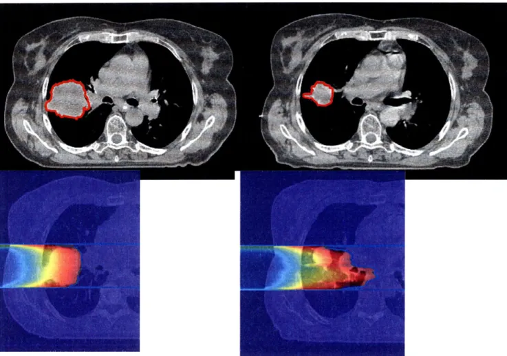
Another source of error is tumor shrinkage. Depending on the type of tumor, the volume may decrease significantly over the course of treatment. (Figure 2-4) As healthy tissue moves into the volume previously occupied by tumor, healthy tissue is exposed to the Bragg peak during treatment. While one possible remedy may be to CT the patient intermittently during treatment, the time and man power required to compare CT images and reevaluate treatment plans multiple times during treatment is unrealistic. The number of patients that would benefit from such work and increased radiation exposure is relatively small (because few tumors shrink to the degree that there is significant overdosing of healthy tissues) compared to the number of patients receiving proton therapy. [Mori, 2007]
Figure 2-4: Lung tumor CT (top) and proton treatment plan (bottom): initial scan, gross tumor volume
(GTV) 115cc (left), 5 weeks into treatment, GTV 39cc (right). Tumor volume hilighted in red. [Mori, 2007]
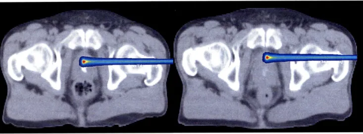
Yet another source of error that is frequently encountered in radiation therapy is patient movement during treatment. The most extreme cases are encountered in thoracic cases (lung, heart, etc.) However, new treatment planning methods and in situ monitoring devices (4D treatment) have reduced the error associated with such movements. Patient movement from treatment to treatment, which results from inconsistent patient positioning is more of a problem. While this if often compensated for by using implanted seeds or pre-treatment X-rays, which use landmarks for proper alignment, the methods are imperfect and misalignments can happen, as demonstrated in Figure 2-5.
Figure 2-5: Prostate Treatment CT 08 Jan 2000 (left) and 11 Jan 2000 (right). Note the rotation of the femoral head and the increased bone traversal length of the beam for 11 Jan. [Chen, 2000]
With such significant sources of error, it is difficult to ensure that the Bragg peak, which has saved thousands of patients' lives and quality of life, does not inadvertently kill healthy tissue in a few patients. Clinicians conservatively add a margin to the tumor volume to account for such uncertainties - this both decreases the potential risk to the patient and reduces the advantages of using a proton beam over more traditional high energy X-rays A quick, reliable and safe means of imaging to ensure that the Bragg peak is being isolated solely to the tumor volume would greatly help to ensure that treatments are being delivered as prescribed and maximize the potential benefits afforded by proton physics.
2.5
CURRENT METHODS FOR IN VIVO PROTON THERAPY
MONITORING
2.5.1 POSITRON EMISSION TOMOGRAPHY
Positron Emission Tomography, or PET, has been around for decades and is a staple of the
nuclear medicine branch of diagnostic radiology. Antimatter, colloquially thought of as the stuff
of science fiction, provides the physical backbone of PET imaging. Positrons are created by
proton rich nuclei, which convert a proton
(p)
into a positron
(P+),
neutron (nU), and a neutrino
(v), plus kinetic energy for the neutrino and the positron.
This positron annihilates when in contact with an electron. Two annihilation photons result, each
with an energy of 51 lkeV traveling antiparallel to each other. These photons which are detected
during PET imaging. [Turner, 2004]
For nuclear medicine applications, a positron emitter is attached to a tracer molecule. Most
commonly,
18F is attached to glucose, resulting in florodeoxyglucose (FDG). Cancers, often
having a higher metabolic rate than surrounding healthy tissue, have a higher uptake of glucose,
which results in a brighter PET signal in the tumor volume. [Cho, 1993]
Once the FDG is injected and allowed to distribute throughout the body, the patient is placed in
a ring of photon detectors (scintillating crystals attached to photomultiplier tubes) which detect
the annihilation photons. [Knoll, 2000] Coincident detection techniques and reconstruction
algorithms are used to determine the origin of each photon pair; higher photon fluence
originating from a particular voxel indicates higher positron emitter concentration. [Cho, 1993]
Positron emitters are also created during proton therapy. As the proton traverses tissue, it mainly
loses energy via collisions with orbital electrons, knocking the electrons out of orbit and creating
6-rays. Less frequently, a proton will collide with a nucleus, which may lead to a multitude of
events; if the proton is of sufficiently low energy it may be absorbed or it may scatter, taking with
it an orbital electron and becoming a hydrogen atom. Occasionally, upon collision with a nucleus,
the proton will knock off a neutron. If this happens to occur in carbon or oxygen (two
commonplace elements in the body) "50 and "C will result, both of which are proton rich,
unstable nuclei that undergo positron decay with halflives of approximately 2 minutes and 20
minutes, respectively. (Figure 2-6) The positrons created from these two isotopes behave
identically to the positrons used for PET imaging. As a result, it is possible to use a standard PET
scanning device to measure the concentration of 150 and
1"C in a particular volume. [Parodi,
Before collision
After collision
Proton 11k
Atomic
nucleus
of
tissue
Target
fragent
Figure 2-6: Schematic of O0 production [Bortfeld, 2008]
There lies a correlation between the energy deposited per mass of tissue and the number of positron emitters created; the PET signal is proportional to the proton fluence and the probability of a proton-nucleus interaction which results in a positron emitter. [Parodi, 2007a] Most importantly, the distal fall-off of the PET signal as a function of depth correlates approximately with the dosimetric distal fall-off of the beam. The PET scan is completed immediately after treatment, providing clinicians with immediate feedback as to the efficacy of the treatment and the deposition of dose by the proton beam. (Figure 2-7)
However, PET verification is not without its drawbacks. The short halflives of the 150 and "C require scanning immediately after treatment. After 20 minutes, the
'~"
signal is essentially zero, and the "C signal has been reduced by a factor of 2. Biological factors affect the signal decay as well - vasculature sweeps activated atoms away from their original irradiation site, ultimately reducing the half life signal and decreasing the signal to noise ratio obtained from scanning. [Parodi, 2007a]-100 .50 -50 -60 50 100 100 too 150 -100 50 0 160 150 50 1 -100 -60 0 50 100 -100 50 0 So 100 mm mm mm
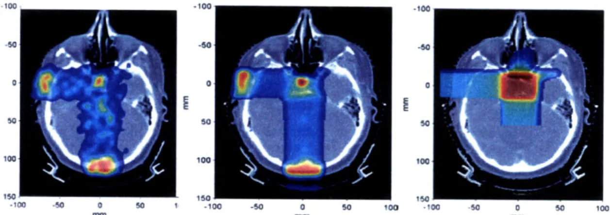
Figure 2-7: Measured PET (left) Monte Carlo PET (middle) and treatment plan dose (right) for a patient with pituitary adenoma receiving two orthogonal fields. [Parodi, 2007b]
The human body is not homogeneous. Tissues have varying composition, and different tissues emit different signal intensities when subjected to the same dose. While this in and of itself is relatively easily compensated for, when taken in conjunction with the biological decay and short-lived isotopes upon which the technique relies, it is difficult to obtain a high SNR image that accurately reproduces the dose profile in the patient. [Parodi, 2007a] The inability to provide a 1:1 correlation between the PET signal and dose has caused most current studies to use PET as a range verification tool, instead of using it to recreate the dose profile, with clinically acceptable levels of uncertainty. [Parodi, 2007b]
2.5.2 POST TREATMENT IRRADIATION MRI OF VERTEBRAL DISCs
Recent studies have shown that spinal proton treatment causes a characteristic pattern of fatty conversion in the vertebral bone marrow that is visible on post treatment MRI scans. [Krejcarek, 2007] Groups have shown that a Tl-weighted hyperintensity of bone marrow from fatty conversion is detectable by the end of radiation treatment and persists for at least 11 months.(Figure 2-8) [Blomlie, 1995] [Cavenagh, 1995] Promising work is being conducted in developing a dose to post-treatment MRI signal intensity curve.
Figure 2-8: Treatment plan (left) Monte Carlo calculation (middle) and MRI (right, blue line is planned 50% isodose line, red line is estimated true 50% isodose line) of lower Lumbar
While the results are promising, the main drawback of this method is the timescale involved. Current studies indicate that the observed TI hyperintensity initially occurs after treatment. As a result, the clinician can not use this information to adjust the patient's treatment. While the information provided is useful for quality assurance and future treatment planning practices purposes, the damage has already been done to the patient at hand by the time the effect is visible.
2.6
INSITU
PROTON RANGE VERIFICATION ASSESSMENT VIA
PROMPT GAMMA DETECTION
While the aforementioned PET and MR methods have yielded some promising results and warrant further research, they have inherent flaws and complications. The effect that biological decay has on the PET signal makes it is difficult to obtain a high SNR representation of the beam range with the PET method. And, while the MRI method provides wonderful data in hindsight, it yields no data in the timeframe necessary for a clinician to change a patient's current treatment plan.
Prompt gamma emission detection has the potential to provide meaningful proton range verification in situ while avoiding some of the pitfalls discussed with other techniques. The technique has the potential to provide instant data to the clinician during treatment, meaning that the data can be analyzed by a clinician after any given fraction, and the remaining fractions can be
adjusted if needed. But information can potentially be gained regarding treatment before the first
fraction is delivered. The high gamma emission rate of approximately 3.5 MBq/mL/Gy,
considerably larger than the PET isotope production rate, may allow clinicians to deliver a
micro-fraction, which would mimic the actual treatment fractions while delivering a small dose to the
patient. This would allow clinicians to monitor the range and ensure compliance with the
treatment plan of the treatment beam before even one fraction was delivered to the patient.
While the data may not be as striking and vivid as the images produced via PET/CT and MRI,
the data are no less useful, and it is this simplicity and the high potential SNR offered by the high
activity rate that make prompt gamma emission detection such a potentially powerful tool.
3
PROMPT GAMMA: BACKGROUND AND INITIAL EXPERIMENTS
3.1
GAMMA DECAY
Gamma emission occurs when a nucleus decays from an excited state to a lower or ground state and emits a photon of energy equal to the difference between the two nuclear states, and is analogous to the emission of characteristic X-rays. [Krane, 1988] In the case of proton therapy, the excited nuclear state results from inelastic scatter between the proton of energy Ep and a nucleus in the material through which the proton is traversing. The proton collides inelastically with the nucleus, scattering with an energy Ep', imparting an energy to the nucleus Enuceus=Ep-Ep' .
This excess energy in the nucleus causes one or more nucleons to enter an excited state. When the(se) excited nucleon(s) return to their ground state, they emit a gamma with energy Ey= Enucleus. This reaction can be described in shorthand as A(p, p' y)A. For example, one reaction that occurs
with carbon is 12C(p, p' 4.44MeV)12C, or
p+12C - p'+ 12*C
12* C 12C
+ Y4.44MeV
Given that nuclei have quantized energy states, such gamma emissions are quantized and particular energies are characteristic of a given nucleus. Table 3-1 describes some of these characteristic gamma rays, and Table 3-2 shows the composition of brain, muscle, water, and polymethyl methacrylate (the latter two being common phantom materials).
Table 3-1: Summary of proton nuclear interactions with the elemental constituents of tissue [Dyer, 1981] [Kiener, 1998]
Isotope Reactions Gamma-ray Energies (MeV)
12C 12C(p, ' y)12C 12C(p,2p y)11B 4.44
14
N 14N(p, p' y)14N 1.64, 2.31, 5.11
Table 3-2: Elemental composition (atom fraction) and density of brain, muscle, phantom materials. [ICRU, 1989]
and representative
Density Elemental Atom Fraction
(g cm-3) H C N O
Brain 1.040 0.646 0.074 0.009 0.271
Muscle 1.014 0.633 0.074 0.015 0.278
Water 1.00 0.667 - - 0.333
PMMA 1.19 0.533 0.333 - 0.133
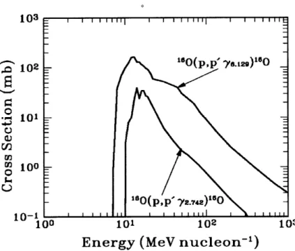
The probabilities of such reactions depend on the energy of the incident proton. The cross section of 6O, for example, has a threshold of 8-10MeV, and a maximum of approximately 0.2 barns. (Figure 3-1)The cross section of "60 is representative of the other reactions listed in Table 3-1.
A typical proton therapy plan administers the proton beam at a rate of approximately 2Gy/min, or 2.1xl1014eV/cm3/g. Dividing by the proton stopping power of approximately 40MeV/cm2/g yields a nominal proton flux of 5.3x10⁹/cm2/s. The inelastic emission rate per unit volume can be estimated as the product of the flux times the cross section (0.2x10⁻²⁴cm) times the number density of the particular nucleus (in this case, 160, 3.34x10²²/cm 3). This results in a gamma emission rate of approximately 3.5 MBq/mL. As tissue composition changes and proton energy decreases along the proton beam path, the rate of emission will vary with depth in target and the emission fluence peak will be slightly proximal to or at the Bragg peak (depending on the initial beam energy), as suggested by the cross section curve in Figure 3-1.
103 102 "DUOp,p y129)u o P- 101 m 10 -0 --- O(p,p' y2.742)'O 10-1I I I I 100 101 102 103
Energy (MeV nucleon-')
Figure 3-1: Proton inelastic scattering cross section for two different characteristic gamma ray lines (6.13MeV and 2.74MeV)
[Kiener, 1998]
3.2
INITIAL KOREAN STUDY
The first study conducted at the National Cancer Center of Korea by Chul-Hee Min et al. used a 100-200MeV proton pencil beam incident upon a water phantom. [Min, 2006] A CsI(T1) scintillator was used to detect the gammas, and was collimated such that only gammas emitted orthogonal to the central axis of the proton beam were registered. The collimator consisted of two parts: a paraffin layer and a lead and B4C layer. The paraffin layer shielded the scintillator
from the high energy spallation neutrons emitted during therapy (which are mostly forward oriented, but strong enough to compete with the photon signal at 900). This paraffin layer moderated the neutrons, the B4C in the lead captured the neutrons by the B(n,y) reaction, and the lead blocked these unwanted gammas. The lead layer also shielded from gammas that are not emitted at 90' and would otherwise taint the signal. (Figure 3-2)
ollimtdon
hole
bstft
4
Bwc
Figure 3-2: Isometric and sectional views of the collimator setup [Min, 2006]
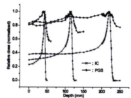
The prompt gamma emission rate correlated strongly with the proton depth dose profile, with a gamma emission peak approximately at the location of the Bragg peak. (Figure 3-3) A significant signal was observed in the plateau region, and the gamma signal dissipated distal to the Bragg peak.
1.0-02
S " I ' I . m I
Depth (m)
200
Figure 3-3: Comparisons of the depth-dose distributions measured by the ionization chamber (for proton dose profile) and the prompt gamma scanner measurement at Ep=100, 150, and 200MeV. Note the slight dip in photon signal slightly proximal to the Bragg peak. [Min, 2006]
3.3
PRELIMINARY EXPERIMENTS AT
MGH
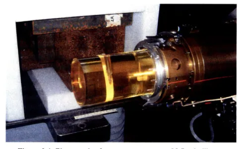
Initial experiments were performed in one of three available therapy rooms at the Francis H. Burr Proton Therapy Center at the Massachusetts General Hospital. In order to minimize the high levels of background radiation that would normally be produced in the treatment room in beam scattering devices used during therapy, measurements were performed using a pencil beam (approximate diameter 5-6mm) with an energy of 150MeV and a beam intensity of 5nA. The beam was incident upon a cylindrical Lucite quality assurance (QA) phantom with a diameter of 10.2cm and a length of 30cm. Gamma rays were measured at 90' to the central axis of the incident beam using a cylindrical 2.5x5cm (diameter x length) Nal scintillator which was coupled to a photomultiplier tube. The detector was collimated with lead bricks, with a wall 10 cm thick and 80cm long, with a slit opening 5mm wide for the detector to view the emitted radiation. (Figure 3-4)
Pulse height data were acquired on a commercial multi-channel analyzer (Canberra industries DSA 1000) and were calibrated using the Compton peaks at 1173 and 1332 keV produced by a
60Co test source. The detector was positioned 52cm from the central axis of the proton beam and
was not shielded from room return scatter or radiation produced upstream in the beam line. The assembly was scanned through the depth of the Bragg peak parallel to the beam direction. A spectrum was acquired at each position for 100 MU of beam dose recorded by the dose monitoring system routinely used during therapy. A monitor unit (MU) is defined as a certain amount of charge collected in an ionization chamber and is a measure of the delivered dose in radiation therapy.
Figure 3-4: Photograph of measurement setup. Nal scintillator
positioned orthogonal to the beamline behind shielding with a 5mm slit aperture (top), scanned along the beam path. Proton beam enters from the right of the image into Lucite phantom (yellow cylinder).
The measured spectrum yielded a gamma emission peak approximately 15mm proximal to the
Bragg Peak, with a relatively large gamma count distal to the Bragg Peak. The gammas distal to
the Bragg peak are attributed to recoil nuclei and neutrons causing activation beyond the proton beam range. The local minima at approximately 18mm proximal to the Bragg Peak is still
unexplained (Figure 3-5), although a similar result was obtained by Min et alin the 225mm range
proton beam shown in Figure 3-3.
120
* Measured gamma emissions
100
-- Calculated absorbed dose (MCNPX)
80 0 C 60 I E . 40 20 0 0 50 100 150 Depth (mm)
Figure 3-5: Gamma emissions measured by Kent Riley and Peter Binns as a function of distance along a Lucite cylinder for an incident 150MeV proton pencil beam plotted with the calculated proton depth dose profile.
4
4.1
EXPERIMENTAL SIMULATION: GEANT vs MCNPX
GEANT 4.8.0
Initial simulations of the MGH experiment described in Section 3.3 were run using the GEANT 4.8.0 radiation transport code developed at CERN. GEANT was chosen because it is the most ubiquitous radiation transport code used by medical physicists in the radiation oncology department at MGH. As a result, a full setup of the proton beam treatment head has been developed and benchmarked in GEANT, and Monte Carlo treatment planning for proton therapy using GEANT is being developed. [Paganetti, 2008]. Initial runs consisted of the full treatment head and Lucite phantom as well as the collimated NaI scintillator (Figure 4-1). Particle-by-particle tracking was conducted on gammas created in the phantom, as well as those that reached the Nal scintillator.
Figure 4-1: Schematic of experimental simulation. Lucite phantom visible as white wireframe cylinder in the lower right. Collimating
blocks visible as purple and green wireframe boxes in the lower right. Upstream proton therapy head components (beam degrader, etc.) visible in the upper left.
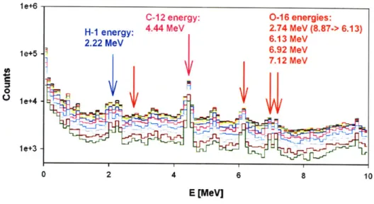
However, initial simulations provided mixed results. The tally of gammas exiting the phantom yielded the characteristic gammas of the materials comprising the phantom, as expected. (Figure 4-2)
le+6 le+5 . 7.12 MeV 0R leI+4e le+3 0 2 4 6 8 10 E [MeV]
Figure 4-2: Spectrum of gammas leaving the Lucite phantom as
calculated by GEANT -Gamma peaks of H, C, and O
highlighted.
The gamma emission profile did not correlate with the proton depth dose profile as had the previous MGH and Korean experiments. Even when energy gating was conducted to examine only characteristic peaks, there was little distinction between the emission profile at and around the Bragg peak and the plateau region of the proton depth dose profile. (Figure 4-3)
0o -0 8e+5 r 6e+5 O c O a- 4e+5 2e+5 C -6 -4 -2 0 2 4 0
o Position relative to Bragg peak (cm)
60000 50000 - 40000 - 30000 S 20000 -10000 -6 -4 -2 0 2 4
Position relative to Bragg peak (cm)
Figure 4-3: Gamma emission profile plotted relative to the Bragg Peak position
A potential cause of this unexpected gamma emission profile was the angular distribution of the emitted gammas. The angular distribution of emitted gammas from a proton beam incident on a phantom (dictated by the angular differential cross section, do/dQ) should be relatively isotropic (indicating that this is an l=0, or S-wave dominated reaction) or have a minima about 900. (Figure 4-4) [Kiener, 1998]
07,12 Mev 60 6.92 Mev E '40 " 300 500 6.13 MeV 4.44 MeV 200 400 0 0000 40 . 2.74 MeV 0 , 2.31 MeV 70
30
-4-
4+-±-50 40 .... 0 50 100 150 0 50 100 150 0,7 (deg.) O, (deg.)
Figure 4-4: Gamma emission angular distribution for Ep=14MeV (the average energy of a proton in the Bragg peak of a 140 MeV beam) on
collodion (C12H16N4018) foils. [Kiener, 1998]
In contrast to this expected angular distribution, the gamma angular distribution varied wildly over the proton beam path, with forward directed gammas at the Bragg peak, backward directed gammas at the entrance region, and a relatively flat angular distribution in the proton plateau region. (Figure 4-5)
0.6-LL 0.4-0 z 0.2 0.0 -1.0 -0.5 0.0 0.5 1.0 Cosine (0) - Entrance Region - Plateau Region SBragg peak
Figure 4-5: Angular distribution of gammas exiting the phantom calculated with GEANT.
Initially it was thought that this may be a problem with the physics packages used with GEANT, but subsequent examination showed that the most up to date physics packages were used for the simulations, and that all angular binning definitions were geometrically correct. The issue is currently under investigation by the Geant4 collaboration.
4.2
MCNPX v2.6.0
-
ANGULAR DISTRIBUTION
Given this problem with GEANT, we decided to examine the angular distribution of gammas with MCNPX, a radiation transport code developed by Los Alamos National Labs. [Pelowitz, 2008] However, MCNPX does not allow for particle-by-particle sampling as GEANT does, so a method had to be developed in order to assess the angular distribution of photons leaving the phantom (ie, we were not able to simply set up an if statement 'if the particle is a photon and exits the phantom, note its trajectory's angle with respect to the proton beam central axis' as we did with GEANT). The phantom was instead divided into regions of Lucite sandwiched between very thin (0.0001cm) void areas with a photon importance of zero. (Figure 4-6)
... .-.-.... . .I p-beam
a b c d e f
Figure 4-6: Schematic of angular distribution geometry in MCNPX. The shaded regions (between surfaces a&b, etc.) have a photon importance of zero. The proton importance throughout is one. White regions have
a photon importance of one. Photons' angular distribution with respect to the proton beam central axis are tallied on each surface. For example, y 1 is tallied on surface c before being killed in the region between c
and d. y2 is tallied on surface g. y3 is tallied on surface d before being killed in the region between c and d.
Not to scale.
The resulting angular distribution calculated by MCNPX was closer to the expected angular
distribution described by Kiener et al with a symmetrical distribution about 90' and a local
minima at 900. (Figure 4-7)
2.50E-04 Bragg Peak -U- Plateau -*- Entrance 2.OOE-04 1.50E-04 5.00E-05 0.OOE+00 -1 -0.8 -0.6 -0.4 -0.2 0 0.2 0.4 0.6 0.8 1 CosineWith these promising results, further benchmarking was undertaken to determine whether
MCNPX could be used to accurately simulate the physics of prompt gamma production from
proton beam therapy.
4.3
MCNPX
-
FURTHER BENCHMARKING
Two measures were used to determine whether the proton and photon physics simulated with
MCNPX were complete enough to simulate the prompt gammas emitted during proton therapy:
proton spectrum in phantom, spectrum of photons leaving the phantom.
4.3.1 PROTON ENERGY SPECTRUM
As the proton traverses a phantom, its energy spectrum should broaden, and at the Bragg peak the average energy should be 10-15% of the original beam energy. At the entrance region, the proton energy spectrum should be approximately that of the source.
0 20 40 60 80 00 120 140 16
Energy (MeV)
Figure 4-8: Energy spectrum of the proton beam calculated by MCNPX at the entrance region (z=0 cm), plateau region (z=5.5 cm), and Bragg peak (z=14.5 cm). Note the energy broadening from a monoenergetic beam at the entrance region to the broad energy range at the Bragg peak.
The proton energy spectrum calculated by MCNPX behaved as expected, with energy range
broadening as the beam loses energy and a peak energy of approximately 10-15% maximum
beam energy at the Bragg peak. (Figure 4-8)
4.3.2 GAMMA ENERGY SPECTRUM LEAVING PHANTOM
We demonstrated that the angular distribution of gammas concurs with published experimental data [Kiener, 1998] (at least in the Bragg peak), but it is also necessary that we demonstrate that the photon energy spectrum is correctly simulated by MCNP in order to thoroughly simulate the experimental setup. The most important features that must be present are the characteristic peaks of carbon, hydrogen, and oxygen.
1.4E-07 - Entrance Region -+- Plateau Region 1.2E-07 -1- Bragg Peak 1.OE-07 U- 8.OE-08 6.OE 08 4.OE-08 2.OE-08 0 0F4-0 0 1 2 3 4 5 6 7 8 9 10
Photon Energy (MeV)
Figure 4-9: Energy spectrum of the gammas exiting the phantom calculated by MCNPX.
As before, a 150MeV proton beam was directed into a Lucite cylinder and the energy spectrum of the exiting photons was recorded. The energy spectrum displayed the expected peaks
-4.44MeV (12C), 2.2MeV ('H), and 6.13 and 7.12MeV (160). (Figure 4-9) This spectrum, combined with the correct angular distribution and the proton energy spectrum provided sufficient
5
HOMOGENEOUS PHANTOM IN MCNPX
5.1
EMULATING THE EXPERIMENTS CONDUCTED AT
MGH
When simulating the experiment previously conducted at the Francis H. Burr Proton Therapy Center by Peter Binns and Kent Riley, it was decided that the simulations would emulate ideal conditions and equipment. As a result, only gammas created by the primary proton beam were tracked. In order to obtain the highest signal possible (which ultimately reduces the error associated with the tallies), an annular ring of sodium iodide (NaI) F4 tallies (flux averaged over the cell) surrounded the Lucite QA phantom. (Figure 5-1) Phantom dimensions were identical to the experimental QA phantom. The Nal tallies were arranged orthogonally to the incident proton beam with an internal radius of 25.1cm, an external radius of 26.1cm, and a width of 1cm. In order to obtain the proton depth dose profile, the QA phantom was divided into segments with a length of 5mm along the proton beam path, each of which contained an F6 tally (energy deposition averaged over a cell).
Figure 5-1: 3-D View of Lucite phantom and annular array of Nal tallies (collimators not shown)
In order to ensure that the tallies registered only photons emitted orthogonal to the proton beam central axis, thin (0.0001cm) ideal collimators were placed between each Nal ring, extending from the phantom to the annular Nal. (Figure 5-1) Tallying was conducted from 0 - 20MeV with increments of 100keV. A 147.5MeV monoenergetic proton pencil beam was delivered to the
Lucite phantom.* Approximately 103 million source particles (protons) were required to obtain uncertainty of <1% for the total gamma fluence detected in the Nal tallies. Run time was approximately 2635 minutes.
ite
Mtom
Nal Tallies
: p beam
Figure 5-2: 2-D View of the phantom (center, red,
diameter=10.2cm), Nal tallies (sides, blue) and collimators (lines extending from phantom to tallies). Proton beam enters phantom from the bottom of the figure. Drawn to scale.
The gamma emission profile yielded a total integral photon emission peak 2±0.5cm proximal to the Bragg Peak, with plateau emissions ranging from 70%-90% of the peak. Spectrographic data from the tallies revealed that the most abundant gamma emission near the Bragg peak was the 4.44MeV peak from 12C, likely due to the high percentage of carbon in Lucite. (Figure 5-3)
* 147.5 MeV proton beam emulates the 150MeV at-nozzle-entrance proton beam used during the experiments. The 150MeV passed through 2m of air, losing approximately 2.5MeV before entering the QA phantom.
8.OE-08
-&-Entrance Region
7.OE-08 -Plateau Region
-- Bragg Peak 6.OE-08 5.OE-08 i 4.0E-08 3.0E-08 2.OE-08 0.OE+00 4 4.1 4.2 4.3 4.4 4.5 4.6 4.7 4.8 4.9 5
Photon Energy (MeV)
Figure 5-3: Energy spectrum of the gammas detected in the annular tallies, 4-5MeV. Note that the fluence at the Bragg peak at 4.5MeV is nearly a factor of 2 greater than other regions of the phantom.
Arbitrary integration about this energy (4-5MeV, as well as 4-8MeV, which was the energy range examined during the initial experiments) was conducted. Both sets of binned data yielded an emission peak at about 1±0.5cm proximal to the Bragg peak, with plateau emissions ranging from 40%-70% and 30%-60% of the peak for the 4-8MeV and 4-5MeV gamma data, respectively. (Figure 5-4)
This difference in peak position relative to the Bragg peak for the total and energy binned data is to be expected - examining Figure 4-9 reveals that there is an abundance of low energy gammas (large 400keV and 600keV peaks) particularly prominent in the plateau region, ultimately raising the number of counts in the plateau region. 4-8MeV and 4-5MeV energy binning discounts these low energy gammas, reducing the number of plateau counts without affecting the number of Bragg peak counts.
The 4-5MeV data yielded the cleanest emission peak, with the highest peak to plateau gamma fluence ratio. However, when compared to the total gamma fluence, narrowing the energy range over which the fluence is integrated lowers the total number of counts received per Gy delivered
![Figure 2-2: Depth dose profile of photons and protons in tissue [Bortfeld, HST.187]](https://thumb-eu.123doks.com/thumbv2/123doknet/14109775.466457/17.918.251.660.773.1039/figure-depth-dose-profile-photons-protons-tissue-bortfeld.webp)
![Figure 2-3: Medulloblastoma treatment plans: photons (top) and protons (bottom) [Bortfeld, HST.187]](https://thumb-eu.123doks.com/thumbv2/123doknet/14109775.466457/18.918.136.730.437.749/figure-medulloblastoma-treatment-plans-photons-protons-bortfeld-hst.webp)
![Table 3-1: Summary of proton nuclear interactions with the elemental constituents of tissue [Dyer, 1981] [Kiener, 1998]](https://thumb-eu.123doks.com/thumbv2/123doknet/14109775.466457/27.918.219.726.823.969/table-summary-proton-nuclear-interactions-elemental-constituents-kiener.webp)