HAL Id: hal-00653289
https://hal.archives-ouvertes.fr/hal-00653289
Submitted on 19 Dec 2011
HAL is a multi-disciplinary open access
archive for the deposit and dissemination of
sci-entific research documents, whether they are
pub-lished or not. The documents may come from
teaching and research institutions in France or
abroad, or from public or private research centers.
L’archive ouverte pluridisciplinaire HAL, est
destinée au dépôt et à la diffusion de documents
scientifiques de niveau recherche, publiés ou non,
émanant des établissements d’enseignement et de
recherche français ou étrangers, des laboratoires
publics ou privés.
Four common conceptual fallacies in mapping the time
course of recognition.
Rufin Vanrullen
To cite this version:
Rufin Vanrullen. Four common conceptual fallacies in mapping the time course of recognition..
Fron-tiers in Psychology, FronFron-tiers, 2011, 2, pp.365. �10.3389/fpsyg.2011.00365�. �hal-00653289�
Four common conceptual fallacies in mapping the time
course of recognition
Rufin VanRullen1,2*
1
Centre de Recherche Cerveau et Cognition, Université Paul Sabatier, Université de Toulouse, Toulouse, France
2
Faculté de Médecine de Purpan, CNRS, UMR 5549, Toulouse, France
Edited by:
Gabriel Kreiman, Harvard Medical School, USA
Reviewed by:
Ryota Kanai, University College London, UK
Gabriel Kreiman, Harvard Medical School, USA
*Correspondence:
Rufin VanRullen, Centre de Recherche Cerveau et Cognition, Pavillon Baudot, Hopital Purpan, Place du Dr. Baylac, 31052 Toulouse, France. e-mail: rufin.vanrullen@cerco. ups-tlse.fr
Determining the moment at which a visual recognition process is completed, or the order in which various processes come into play, are fundamental steps in any attempt to under-stand human recognition abilities, or to replicate the corresponding hierarchy of neuronal mechanisms within artificial systems. Common experimental paradigms for addressing these questions involve the measurement and/or comparison of backward-masking (or rapid serial visual presentation) psychometric functions and of physiological EEG/MEG/LFP signals (peak latencies, differential activities, single-trial decoding techniques). I review and illustrate four common mistakes that scientists tend to make when using these paradigms, and explain the conceptual fallacies that motivate their reasoning. First, contrary to collec-tive intuition, presentation times, or stimulus-onset asynchrony masking thresholds cannot be taken to reflect, directly or indirectly, the timing of relevant brain processes. Second, psychophysical or electrophysiological measurements should not be compared without assessing potential physical differences between experimental stimulus sets. Third, such comparisons should not be performed in any manner contingent on subjective responses, so as to avoid response biases. Last, the filtering of electrophysiological signals alters their temporal structure, and thus precludes their interpretation in terms of time course. Practical solutions are proposed to overcome these common mistakes.
Keywords: visual timing, methodological and conceptual mistakes, EEG, backward-masking, rapid serial visual presentation, low-level image properties, response bias, signal filtering
INTRODUCTION
A major portion of vision science is devoted to investigating the timing of perceptual processes: the absolute latency or the rela-tive order in which they arise after a novel object enters the visual scene or after we open our eyes onto a novel scene. This is the main subject covered in the various companion articles published in this Special Topic. Example questions include: how long does it take the visual system to detect, recognize, categorize, or identify an object? how long to get the gist of the scene, and how long for a detailed analysis? do detection and categorization processes happen sequentially, or all at the same time? how about differ-ent levels of categorization? For each of these questions, there exist many experimental approaches relying on psychophysical measurements and sometimes accompanied by recordings of elec-trophysiological activity. Having published on these questions for the last 12 years or so, I am often asked to review novel findings in this field. In this process, I started noticing a small number of technical and conceptual errors that appear to come back repeat-edly. I can see at least two reasons behind this. The first possible reason is that these mistakes have been committed and the corre-sponding results published in the past, sometimes in high profile journals – encouraging new authors to pursue in the same direc-tion. The second reason is that there exists no formal, citable report warning authors against these faulty rationales. While nothing can be done about the first reason (and throughout this man-uscript I will purposefully avoid referring to specific published studies as examples of guilty reasoning), the present manuscript
is an attempt at correcting the second reason. I will insist on four common mistakes, listed here by decreasing order of conceptual importance, frequency of occurrence, and generality: (i) confusing stimulus presentation time and processing time; (ii) comparing experimental conditions with systematic physical differences in stimulus sets; (iii) comparing experimental conditions contingent on subjective responses; and (iv) filtering of electrophysiological signals.
MISTAKE #1. CONFUSING STIMULUS PRESENTATION TIME AND PROCESSING TIME
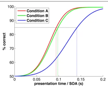
One scientist measures that a stream of rapidly changing images (rapid serial visual presentation or RSVP) can be “processed” (e.g., recognized or classified) up to a rate of 10 images per second, and concludes that “processing” takes the visual system about 100 ms. Another scientist measures that backward-masking (flashing a powerful “mask” shortly after a target “stimulus”) prevents process C, but leaves both processes A and B unaffected when stimulus-onset asynchrony (SOA) between the stimulus and the mask is about 100 ms (Figure 1). In turn, process C can be performed effi-ciently, but only when enough presentation time is given before mask onset, i.e., with SOAs above 150 ms. This scientist concludes that process C takes the visual system about 50 ms longer to com-plete than processes A and B, and that these two have comparable time courses.
Intuition suggests that the findings of these two scientists are valid and worthy of publication. In fact, peer review has followed
VanRullen Fallacies in time course experiments
FIGURE 1 | Psychometric functions (hypothetical) for a typical RSVP or masking experiment. The x -axis would represent presentation time of
each image in the sequence, or stimulus-mask SOA (respectively). The natural tendency to read from this graph that processes A and B have similar speeds whereas process C is 50 ms slower is inaccurate. See text for explanation.
this intuition (in at least some documented cases), and the above-mentioned arguments have been printed in forefront scientific journals. Again, the purpose of this paper is not to point at spe-cific past instances of the mistakes listed, but rather to avoid their re-occurrence in the future; therefore, no citation to faulty publi-cations will be provided here (names of brain processes and their corresponding latencies have been altered, all resemblance to exist-ing findexist-ings is fortuitous). What could possibly be wrong with their apparently flawless logic?
First, it is easy to see that processing N images per second does not imply a processing duration of 1/N second. Indeed, in certain situations the brain has been reported to “process” (more specifically, detect the presence of a face) up to 72 images per second (Keysers et al., 2001). (Note: citations will of course be provided in this manuscript, but only when the corresponding methodology or interpretation are free of the alleged mistakes). Pushing the previous reasoning would result in the conclusion that this process takes the brain about 14 ms, and therefore cul-minates at the level of retinal ganglion cells! The fallacy of this reasoning is best illustrated by a simple metaphor: a car factory can produce one new car every minute, yet it does not take 1 min to produce a car! Just in the same way, considering the visual system’s hierarchy as a “pipeline” (or an assembly line, to follow the metaphor) can help explain how the brain can process a new image every few 10 ms, when visual discrimination processes actu-ally take hundreds of milliseconds: it is the time spent at each stage of the pipeline that limits the processing rate, not the cumulative time for all stages.
What of the second scientist? If absolute statements about pro-cessing duration are subject to erroneous logic, purely relative statements should at least be immune to it: this scientist should be allowed to compare processes A, B, and C and conclude that
the latter takes 50 ms longer than the other two. Right? In fact, not. Presentation times (or SOAs) directly affect the amount of information (or the “signal-to-noise”) that reaches the earliest lev-els of visual representation; it is always possible that one process requires more “information” to complete than another, yet the two processes proceed at the same exact speed. Think of a camera tak-ing pictures, and a computer processtak-ing these pictures; when the camera shutter opens for a very short time, the computer may not be able to perform certain functions that it could have per-formed easily with longer shutter opening times (i.e., with more input signal-to-noise); however, when signal-to-noise is sufficient, all these functions may take exactly the same processing time to the computer (e.g., in terms of clock cycles). In other words, stimulus presentation time is better likened to a measure of information, than to a measure of processing duration.
PRACTICAL SOLUTIONS
If you must use RSVP or masking psychometric functions to com-pare two brain processes, do not draw any conclusion in terms of their duration, or the relative order in which they are completed. The only safe conclusion when two psychometric functions are found to differ is that the two processes cannot be equated, and thus rely (at least in part) on distinct neuronal mechanisms. Of course, no conclusion can be drawn if the psychometric functions do not differ – the underlying processes may still differ in other respects.
Other psychophysical methods can be better suited to the com-parison of processing times between different conditions. For example, comparing reaction times is rather safe: assuming that purely motor components do not change significantly, a difference in reaction times can be taken to reflect a difference in the tim-ing of completion of each process. Here again, there are dangers to avoid: for example, the mean reaction time is generally not a good measure, because it is not representative of a skewed reaction time distribution. Working with the entire distribution, or using only the fastest (significantly above chance) responses, are viable options (Fabre-Thorpe et al., 2001;VanRullen and Thorpe, 2001a; Rousselet et al., 2002;Mace et al., 2005).
Finally, there exists no psychophysical method that can provide a measure of absolute rather than relative process duration. Here again, reaction times can at least prove useful in providing an upper limit for this duration. For example, using saccadic eye movements (a response with a very short and automatic motor component), Thorpe and colleagues estimated that certain natural scene clas-sifications can be performed in less than 120 ms (Kirchner and Thorpe, 2006;Crouzet et al., 2010; see also Thorpe and Crouzet in this Special Topic). In order to pinpoint the precise latency of a given brain process rather than just an upper limit, one should turn to electrophysiological rather than psychophysical methods.
MISTAKE #2. COMPARING STIMULUS SETS WITH SYSTEMATIC PHYSICAL DIFFERENCES
In a typical experiment, electrophysiological responses (say, EEG) are recorded for two classes of images differing along a critical dimension (e.g., faces vs. other objects, familiar vs. non-familiar faces, animal vs. non-animal scenes, etc.). Subtle but significant differences in event-related potentials (ERPs) between the two
conditions are interpreted as the signature of neuronal mecha-nisms that are capable of distinguishing between them (i.e., of recognizing faces, or detecting animals). A more recent variant of this class of experimental paradigms consists in applying mul-tivariate decoding methods to the electrophysiological signals, in order to reveal the moment at which the brain is capable of discriminating the stimuli.
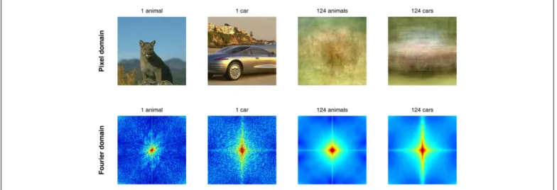
In many cases these approaches rely on the diversity of the image set as a guarantee that the effects are due to true classifi-cation, rather than a trivial low-level cheat of the visual system. The underlying logic is more or less as follows: if it was always the same face and always the same object presented to the observers, then a low-level trick could suffice, but so many different faces and objects were used that any simple trick should fail to differenti-ate them all. Right? In fact, not. First, systematic differences exist between various natural image classes (see Figure 2 for examples of information available in the pixel domain and in the Fourier domain), and it has been shown that these differences can allow a simple classifier (i.e., a low-level “trick”) to discriminate between image classes with 80–90% accuracy (Oliva and Torralba, 2001). Second, the observers may be classifying the images at 95% correct or more, but it is the neuronal signals under study, not the sub-ject’s behavior, that should be pitted against the null hypothesis of a low-level “trick.” If differential ERP activities are considered at their earliest latencies (when they are just reaching statistical significance, and represent only a small proportion of the ERP itself), if multivariate decoding performance is also around 80 or even 90% correct (just like low-level image classifiers), then there is always a risk that the observed signals were simply a reflection of small but systematic physical differences in the stimulus sets. PRACTICAL SOLUTIONS
The confounds described cannot be simply discarded by assuming that “physical differences are unlikely to account for the observed effects” (a phrase often encountered in author correspondence or
even in certain published manuscripts). Rather, the physical dif-ferences should, at least, be quantified or, even better, eliminated. For example,Honey et al. (2008)created meaningless images (ran-domized phase spectrum) possessing the power spectrum of face images (low-level oriented energy information) to show that the natural tendency of observers to move their gaze toward faces was in fact a consequence of low-level image properties. This question is discussed more fully in a recent article byCrouzet and Thorpe (2011), as part of this same Special Topic. Another example is a study byRousselet et al. (2008)who used a para-metric approach (general linear model) to quantify the influence of various physical descriptors for natural images (skewness and kurtosis of the pixel value histogram, Fourier phase spectrum) on the amplitude of the EEG at various delays post-stimulus. Well-controlled studies are now made widely accessible even to authors with no prior image processing expertise, thanks to certain soft-ware packages and libraries. For example, a wavelet-based softsoft-ware byPortilla and Simoncelli (2000)allows one to synthesize textures (i.e., meaningless images) matched to a given target image along several statistical dimensions. A recent MATLAB toolbox by Wil-lenbockel et al. (2010)permits matching two images or image sets in terms of several low-level properties: luminance, contrast, pixel histogram, Fourier amplitude spectrum.
Arguably, this brief survey fails to encompass the complexity of the problem. There are many different ways of attempting to compare images based on “low-level” properties and there is a whole field of papers dealing with computer vision and compu-tational neuroscience modeling approaches to image recognition. Normalizing or eliminating level” confounds, where “low-level” is not always clearly defined, is easier said than done. Still, authors will gain by attempting to tackle the problem, rather than pretending it does not exist.
Finally, it is worth mentioning that physical differences between two image classes can sometimes be eliminated by interchang-ing their task-related status in different experimental blocks (e.g.,
FIGURE 2 | Low-level differences exist between image classes in the pixel and in the Fourier domains. These confounds are systematic enough
to allow distinguishing between images containing animals or cars, for example. As can be seen in the two columns on the right, the average of 124 pictures of animals (including mammals, birds, reptiles, fish) itself resembles
(a “hazy” view of) an animal, whereas the average of 124 cars is much more similar to a car picture. The same can be said of averages in the Fourier domain (bottom). A simple “detector” or “classifier” using the two patterns on the right as templates would easily distinguish between the two examples on the left, without any need for feature, object, or category representations.
VanRullen Fallacies in time course experiments
target or distractor in a go/no-go task). With this approach, Van-Rullen and Thorpe (2001b) demonstrated that although brain signals can “distinguish” between natural image categories as early as 70–100 ms post-stimulus, the true categorization of an image as target or distractor does not happen until 150 ms post-stimulus. One obvious advantage of this method is that it requires no image processing whatsoever (only twice the number of experimental trials, since each image category must be presented once as target, and once as distractor).
MISTAKE #3. COMPARING EXPERIMENTAL CONDITIONS CONTINGENT ON SUBJECTIVE RESPONSES
Let us assume that our favorite scientist has now learned her les-son, and is contrasting the brain signals elicited by two classes of images that have been carefully controlled for systematic low-level differences. In her comparison, this scientist decides to include only the correct trials: surely if the observer was not able to recog-nize or categorize the picture on a given trial, including this trial in the analysis would only add noise, but not help reveal the brain correlates of recognition/classification. Right? In fact, not.
Allow me another example. A second scientist boldly attempts to isolate the brain correlates of the conscious perception of a stim-ulus. During a task in which the target stimulus is difficult to detect (thanks to a masking procedure, or to short presentation times, low contrast, etc.), the scientist will sort the experimental trials according to the observer’s subjective report: did they perceive the target on this trial or not? A brain signal that would be present for detection but absent otherwise would constitute a good candidate for a “neural correlate of consciousness.” Right? In fact, not.
The problem is very similar in these two examples, but may be more easily understood with the second. In the (hypothetical) experiment described, the stimulus was the same on every trial, and only the subject’s perception changed. Comparing the two outcomes (perceived vs. unperceived) should, in theory, isolate the brain signals that were elicited by conscious perception. However, let us assume for a minute that the subjects’ reports are not direct and dependable markers of perception: sometimes, the subject simply did not know or did not see very well (or was not pay-ing attention to the task), and ended up makpay-ing a response based on whatever information was at hand. For example, on these few trials (maybe only 10% of the total) the subject responded “per-ceived” whenever frontal lobe activity around the expected time of stimulus onset was high, and “unperceived” when it was low. Contrasting perceived and unperceived trials should now logically give rise to a positive difference in frontal electrodes. Even if the proportion of trials contributing to this effect is low, with enough signal-to-noise (i.e., a sufficient total number of trials) the differ-ence will turn out significant. Depending on which activity period was used by the brain to make up the response on these trials, one may then be drawn to conclude that frontal brain activity at 100 ms, or even just 50 ms post-stimulus, or even before stimulus
onset, is a correlate of conscious perception. In a recent study, we
actually demonstrated that the phase of a frontal 7–10 Hz oscilla-tion at a given moment can determine (to some extent) whether a stimulus presented 100 ms later will be reported by the sub-ject as consciously perceived or not (Busch et al., 2009). It is easy in this situation to avoid committing the mistake of calling such
pre-stimulus activity a “neural correlate of conscious perception.” But what if the peak of this oscillatory effect had been observed at 100 or 200 ms post-stimulus? The conclusion that this activ-ity contributes to the neural correlates of consciousness may have been more easily accepted – but it would still be logically wrong!
What of our first scientist? Similarly, her restricting the analysis to correct trials could have introduced response biases into the results. The logic is a little more difficult to follow in this case, so I ran a simple simulation to convince the reader (Figure 3). Assume again that on a certain number of trials (even as low as 10%), because of a momentary lapse of attention or a failure of perception, the urge to press response button A or B (for a sim-ple categorization task) is determined not by stimulus properties (category A or B) but merely by the level of activity somewhere in the brain, say a frontal area: when activity is high, the sub-ject will tend to press button A, when it is low they will press button B. Comparing images from categories A and B that were correctly categorized leads to a bias: certain correctly categorized images of type A (maybe only 10%) will tend to be accompanied by high activity in frontal brain regions, certain images of type B being accompanied by low activity. Of course, there is normally an equivalent number of type A images that should be accompa-nied by low activity, and type B images with high activity – but these were purposefully removed from the analysis, because they were “incorrectly” classified! The net result is a purely artifactual difference between the two experimental conditions. As in the pre-vious example, depending on which activity period was used by the brain to make up the response, this difference could conta-minate the “correlates of categorization” as early as 100 or 50 ms post-stimulus, or even before stimulus onset (see Figure 3). In this latter case, the mistake would be easily detected, but the presence of such a difference at 50 or 100 ms post-stimulus could well be construed as a meaningful result – erroneously.
PRACTICAL SOLUTIONS
In order to understand how to avoid such mistakes, let us con-sider what was common between the two examples described. In both cases, the scientists recorded brain signals (e.g., frontal lobe EEG) and used these as temporal markers for the completion of specific neural decision processes (e.g., categorization, conscious perception). What went wrong was due to the fact that neural decision processes indeed modulate the amplitude of brain signals recorded by the experimenter, but sometimes the amplitude of certain brain signals can also contribute to determine the appar-ent outcome of these neural decision processes. In a nutshell: if the causal relation between neural decision processes and brain signals can go in both directions, using one (the brain signal) as a temporal marker for the completion of the other (the neural decision process under study) is, to say the least, dangerous. One simple way to avoid these dangers is to restrict data analyses to the comparison of experimental conditions as manipulated by the experimenter (e.g., stimulus categories A vs. B), without ever tak-ing into account subjective responses. In our two examples, the scientists did not follow this rule: they compared category A
con-tingent on response A to category B concon-tingent on response B (first
example) or simply, response A to response B (second example). As soon as subjective responses are entered into the comparison, the
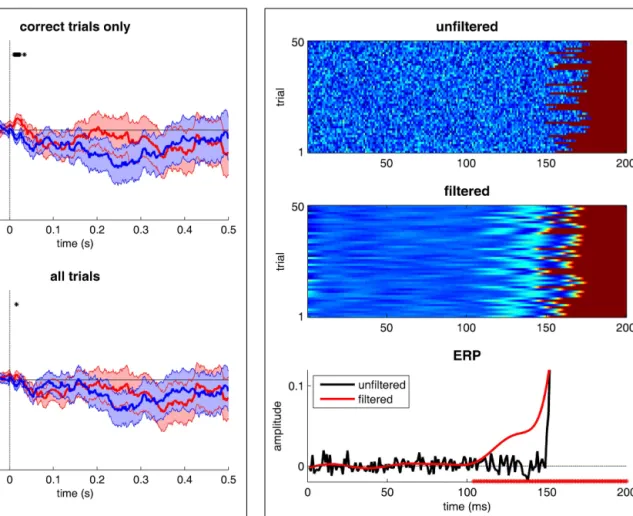
FIGURE 3 | Taking into account subjective responses when contrasting brain signals can generate spurious differences. 1000 trials were
simulated, half of them with a stimulus from category A and the other half from category B. For the purpose of demonstrating the existence of response biases, each EEG waveform was drawn randomly with a 1/f power spectrum, thus approximating the statistics of natural EEG but without any selective response evoked by category A or B. Hence, we should normally expect to obtain flat event-related potentials (ERPs, computed by averaging all trials of each category, with each trial baseline-corrected using the period [−50, +50 ms] around stimulus onset). We assume that the observer correctly categorizes 75% of all trials, but on the remaining 25%, the observer decides to respond not on the basis of the stimulus category (A or B), but based on EEG activity during the 200-ms pre-stimulus period: when the average pre-stimulus activity is positive, the observer presses response button A, and button B when the activity is negative. Of course, negative or positive pre-stimulus activity is equally likely to occur regardless of stimulus type, and therefore the ERPs obtained for stimulus categories A (in blue) and B (in red) will be statistically indistinguishable (bottom panel). However, when only the correct trials are included in the ERPs, many trials with negative pre-stimulus activity and response A and many trials with positive pre-stimulus activity and response B will be discarded from the ERPs (because they correspond to “incorrect” categorization). As a result, the ERPs will show a purely artifactual but significant difference during the pre-stimulus period (top panel).
possibility of an ill-defined causal relation between brain signals and neural decision processes can introduce response biases and obscure data interpretation. These biases, however, cannot be exposed using classic signal detection theory methods, in which the bias denotes an overall tendency to favor one response over the other (e.g., response A over B): indeed, the kind of bias that we
FIGURE 4 | The dangers of filtering. 50 trials of a “fake” EEG signal were simulated. Activity is null until the “onset” of a neural process, occurring at
a random time between 150 and 180 ms (uniform distribution), after which activity is set to 1. Gaussian-distributed noise (mean 0 and SD of 0.05) is added to all signals. In the top panel, the original trials are stacked vertically and the EEG amplitude is color-coded. The middle panel represents the same trials after low-pass filtering with a 30-Hz cut-off (using the function eegfilt from the EEGLAB software, and its default parameters). The bottom panel illustrates the corresponding ERPs. The red∗ symbols on the horizontal axis indicate the moments at which the filtered ERPs depart from zero. Even though, by design, the process under study never started before 150 ms, its EEG correlates are detected with latencies as early as 100 ms!
are discussing would be conditional on the value of certain brain signals, and there may be no apparent overall response bias. It is up to the experimenter to consider what sort of biases could arise, and whether their analysis will be immune to such bias. As a rule of thumb, comparison between two classes of stimuli presented to an observer in interleaved trials, without any subsequent trial selection based on response type or correctness, should be free of these response biases; on the other hand, such comparisons may not be free of stimulus-induced low-level confounds, as developed in the preceding section! The solution of interchanging target and distractor status for two (or more) stimulus categories, which we described in the previous section, could also apply here, i.e., it would be immune to response biases (if all trials are considered, not just the correct trials) and of course to low-level confounding factors.
VanRullen Fallacies in time course experiments
MISTAKE #4. FILTERING OF ELECTROPHYSIOLOGICAL SIGNALS
The last mistake is one that is easy to understand, yet often occurs in the electrophysiological literature. It is common practice when dealing with EEG signals (or MEG, LFP, etc.) to low-pass filter the signals in order to temporally “smooth” them and remove the “noise” – which is generally considered to be proportion-ately most manifest at higher frequencies. Many classic studies list in their Methods section a cut-off frequency of 40 Hz or even 30 Hz. While this is mostly harmless for studies interested in the amplitude or even the latency of specific ERP peaks (in technical terms, because these filters have “zero phase-lag”), it can be extremely problematic when assessing the precise tim-ing and dynamics of brain processes. Indeed, because of the width of the filters used, the EEG correlates of a given neu-ronal event will be smeared out in time for several tens or even hundreds of milliseconds before and after the event. As illus-trated inFigure 4, a neuronal process that actually starts between 150 and 180 ms post-stimulus can appear to start as early as 100 ms, after a simple 30 Hz low-pass filter is applied. When it comes to determining the time course of visual recognition processes, mistakes of this magnitude are sure to have drastic consequences.
PRACTICAL SOLUTIONS
For such a simple ailment there is a simple remedy: raw data should be analyzed directly, without filtering (of course, artifact rejection
can still be applied whenever appropriate). If filtering must be used, then the authors should be careful to restrict their interpre-tations to the quantification and comparison of peak amplitudes and latencies – but not examine onset latencies or precise tem-poral dynamics. Note, however, that this problem only concerns filters with low-pass frequencies in a range likely to correspond to physiologically meaningful time scales (as a rule of thumb, lower than 100 Hz): for example, many EEG amplifiers use built-in low-pass filters with cut-off frequencies at 1 kHz or higher, and although these could theoretically distort neuronal onset latencies by 1 or 2 ms, most experimental conclusions would be unlikely to be significantly affected.
CONCLUSION
We reviewed four important conceptual mistakes that often re-occur in the psychophysical and electrophysiological literature on visual timing. There are certainly many other possible pitfalls in studying the timing of visual recognition. My own previous stud-ies (and likely, my future ones) are probably also not exempt of conceptual mistakes. The list of mistakes presented here was not intended to be exhaustive, nor the proposed solutions to encompass all possibilities. The present aim was, merely, to alert colleagues about the existence of these fallacies, and to provide them with a source and a reference. Hopefully this work will help prevent perpetuating these four mistakes on the grounds that “this is how things have always been done” and “no-one ever said it was wrong.” Now, you know.
REFERENCES
Busch, N. A., Dubois, J., and VanRullen, R. (2009). The phase of ongoing EEG oscillations predicts visual percep-tion. J. Neurosci. 29, 7869–7876. Crouzet, S. M., Kirchner, H., and
Thorpe, S. J. (2010). Fast saccades toward faces: face detection in just 100 ms. J. Vis. 10, 16.11–16.17. Crouzet, S. M., and Thorpe, S. J. (2011).
Low-level cues and ultra-fast face detection. Front. Percept. Sci. 2:342. doi:10.3389/fpsyg.2011.00342 Fabre-Thorpe, M., Delorme, A., Marlot,
C., and Thorpe, S. (2001). A limit to the speed of processing in ultra-rapid visual categorization of novel natural scenes. J. Cogn. Neurosci. 13, 171–180.
Honey, C., Kirchner, H., and VanRullen, R. (2008). Faces in the cloud: Fourier power spectrum biases ultrarapid face detection. J. Vis. 8, 9.1–9.13. Keysers, C., Xiao, D. K., Foldiak, P.,
and Perrett, D. I. (2001). The speed
of sight. J. Cogn. Neurosci. 13, 90–101.
Kirchner, H., and Thorpe, S. J. (2006). Ultra-rapid object detection with saccadic eye movements: visual pro-cessing speed revisited. Vision Res. 46, 1762–1776.
Mace, M. J., Richard, G., Delorme, A., and Fabre-Thorpe, M. (2005). Rapid categorization of natural scenes in monkeys: target predictability and processing speed. Neuroreport 16, 349–354.
Oliva, A., and Torralba, A. (2001). Mod-eling the shape of the scene: a holistic representation of the spa-tial envelope. Int. J. Comput. Vis. 42, 145–176.
Portilla, J., and Simoncelli, E. P. (2000). A parametric texture model based on joint statistics of complex wavelet coefficients. Int. J. Comput. Vis. 40, 49–71.
Rousselet, G. A., Fabre-Thorpe, M., and Thorpe, S. J. (2002). Parallel
processing in high-level categoriza-tion of natural images. Nat. Neurosci. 5, 629–630.
Rousselet, G. A., Pernet, C. R., Ben-nett, P. J., and Sekuler, A. B. (2008). Parametric study of EEG sensi-tivity to phase noise during face processing. BMC Neurosci. 9, 98. doi:10.1186/1471-2202-9-98 VanRullen, R., and Thorpe, S. J. (2001a).
Is it a bird? Is it a plane? Ultra-rapid visual categorisation of natural and artifactual objects. Perception 30, 655–668.
VanRullen, R., and Thorpe, S. J. (2001b). The time course of visual pro-cessing: from early perception to decision-making. J. Cogn. Neurosci. 13, 454–461.
Willenbockel, V., Sadr, J., Fiset, D., Horne, G. O., Gosselin, F., and Tanaka, J. W. (2010). Control-ling low-level image properties: the SHINE toolbox. Behav. Res. Methods 42, 671–684.
Conflict of Interest Statement: The
author declares that the research was conducted in the absence of any commercial or financial relationships that could be construed as a potential conflict of interest.
Received: 01 July 2011; accepted: 21 November 2011; published online: 07 December 2011.
Citation: VanRullen R (2011) Four com-mon conceptual fallacies in mapping the time course of recognition. Front. Psychol-ogy 2:365. doi: 10.3389/fpsyg.2011.00365 This article was submitted to Frontiers in Perception Science, a specialty of Frontiers in Psychology.
Copyright © 2011 VanRullen. This is an open-access article distributed under the terms of the Creative Commons Attribu-tion Non Commercial License, which per-mits non-commercial use, distribution, and reproduction in other forums, pro-vided the original authors and source are credited.