Closed-loop controlled filament stretching and break-up of polymer solutions

Closed-loop Controlled Filament Stretching

and Break-up of Polymer Solutions

by

Roger Yeh

Bachelor of Science in Mechanical Engineering

and Applied Mathematics

Massachusetts Institute of Technology, 2002

Submitted to the Department of Mechanical Engineering

in partial fulfillment of the requirements for the degree of

Master of Science in Mechanical Engineering

at the

MASSACHUSETTS INSTITUTE OF TECHNOLOGY

June 2005

@Roger Yeh, MMV. All rights reserved.

The author hereby grants to MIT permission to reproduce

and distribute publicly paper and electronic copies

of this thesis document in whole or in part.

A u th o r

...

.

...d... ...

Depart

t of Mechanical Engineering

A If r ₄

,4, M

_\ay

_{21, 2005}

Certified by ...

.

Professz f

GartJH. McKinley

Mechanical Engineering

Thesis Supervisor

Accepted by ...

.

...

Lallit Anand

Professor of Mechanical Engineering

Chairman, Department Committee on Graduate Students

OF TECHNOLOGY

Closed-loop Controlled Filament Stretching

and Break-up of Polymer Solutions

by

Roger Yeh

Submitted to the Department of Mechanical Engineering on May 21, 2005, in partial fulfillment of the

requirements for the degree of

Master of Science in Mechanical Engineering

Abstract

A constant true (radial) strain rate filament stretching experiment has been the

Holy Grail of extensional rheological studies. These experiments are performed on a Filament Stretching Extensional Rheometer (FiSER). A filament stretching ex-periment is the only direct way of measuring the extensional viscosity of a fluid. Previous attempts to achieve constant rate stretching have required tedious and it-erative processes, which relied on the data of previous experiments to generate an axial profile that would result in a constant true strain rate experiment. This study presents a method to actively control the axial strains via the utilization of radial strain feedback. The first method we tried was an "Euler 1st order approximation," in which the ratio of the axial and radial strains is calculated at each time-step to determine the axial strain necessary at the next time-step to maintain a constant ra-dial strain rate. This method worked, but was limited by how accurate this "ratio" of strains could be calculated. The "ratio" becomes unstable when the change in strain per time-step reaches the same order of noise. To fix this problem, we implemented a least squares linear regression scheme. With this algorithm, we were able to reach radial strains of ED - 7 with strain rates of 0.8 < D < 5 s-1.

Finally, we compared stretch-to-break (STB) experiments of a Newtonian fluid, styrene oil, to theoretical model. These experiments are also done on FiSER with the nominal strain rate held constant, generally very low ( D - 0-1 s-1). For a Newtonian

fluid, the diameter decay can be determined analytically. We repeat the same with a weakly elastic fluid, STP@ motor oil.

Thesis Supervisor: Gareth H. McKinley Title: Professor of Mechanical Engineering

Acknowledgments

There have been many people who have helped me throughout my academic career. Many thanks to all of them. I would particularly like to thank my family, especially my mom and sister, for all their love and support. My good friends Brian, Grace, and Allen, were the best cheerleaders that no money can buy. My labmates in the Non-Newtonian Fluids group, especially Trevor and Giorgia, were very helpful in providing insight to my research as well as stress relief. Additional thanks goes to Fred in the Edgerton machine shop for putting up with me through all these years. May he finally "retire" for real. Finally, I want to thank my advisor, Gareth McKinley, for giving me the opportunity to work on this project. His guidance was vital in the progression and success of this study.

Contents

Abstract 3 Acknowledgements 5 Table of Contents 9 List of Figures 13 List of Tables 15 1 Introduction 17 2 Literature Review 21 2.1 Elongational Flow . . . . 21 2.2 M echanics . . . . 23 2.2.1 Kinematics . . . . 24 2.2.2 Dynamics . . . . 26

2.3 Kinetic Theory of Visco-elastic fluids . . . . 27

2.3.1 Coarse Graining . . . . 27

2.3.2 Bead-rod and Bead-spring Models . . . . 28

2.3.3 Rouse Model . . . . 30

2.3.4 Zimm model . . . . 31

2.4 FENE Models . . . . 32

2.4.1 FENE-PM . . . . 33

2.4.3 Comments on FENE-PM ... 37 2.5 _{Dimensionless Groups . . . . 38} 3 Filament Stretching ₄₁ 3.1 _{H ardw are . . . . 41} 3.1.1 Linear Motor . . . . 41 3.1.2 Laser Micrometer . . . . 43 3.1.3 Force Transducer . . . . 44 3.2 _{Force Balance . . . . 48}

3.3 Capillary Thinning and Break-up Experiments . . . . 51

3.4 Stretch-to-Break (STB) Experiments . . . . 52

3.5 Filament Stretching Extensional Experiments . . . . 54

4 Control Schemes for Filament Stretching Experiments 59 4.1 Previous Work _{. . . . 59}

4.1.1 Adaptive Control . . . . 62

4.2 _{Euler Method . . . . 64}

4.2.1 _{Noise Problems . . . . 66}

4.3 Least Square Approximation . . . . 67

4.4 Other Considerations . . . . 68

4.5 Other Closed-Loop Methods . . . . 70

5 Rheology of a Dilute Polymer Solution ₇₃ 5.1 Fluid - _{PS025 . . . . 73}

5.2 Shear Rheology . . . . 74

5.2.1 Oscillatory Shear Flow . . . . 77

5.3 Extensional Rheology . . . . 78

5.3.1 _{Type II Results . . . . 80}

5.3.2 Type III Results via Euler . . . . 83

5.3.3 Type III Results via Least Squares Approximation . . . . 85

5.4 Lubrication Effects on Initial Conditions . . . . 90

6 Break-up of Newtonian and Weakly Elastic Fluids 93 6.1 A Proposed Theoretical Model . . . . 93

6.2 STB Experiments with Styrene Oil . . . . 95

6.3 STB Experiments with STP Oil . . . . 98

7 Conclusions 103 7.1 Filament Stretching Type II Experiments . . . . 103

7.2 Filament Stretching Type III Experiments . . . . 104

7.3 Newtonian Break-up Experiments . . . . 104

7.4 Final Comments . . . . 105

A Appendix 107 A .1 Sam ple Code . . . . 107

List of Figures

1-1 Examples of break-up phenomena. . . . . 19

2-1 A fluid sample, simplified as a cylindrical body, being stretched

uni-axially. . . . . 21

2-2 The endplate separation, L, and mid-plane diameter, D, of a fluid sample being stretched. . . . . 24

2-3 The master curve for a filament stretching experiment. . . . . 26

2-4 The various levels of coarse-graining in polystyrene (M ~ 2.25 x 106 g/m ol). . . . . 29 2-5 Deformation components, Azz,j and Arr,i, of the FENE-PM model for

a strain rate of = 1 s-1. . . . . 3 4 2-6 The effect of changing the number of modes used in the FENE-PM

model on the total polymer stress. . . . . 35 2-7 Total fluid stress, as predicted by FENE-PM. . . . . 35 2-8 Total fluid stress for a stretching experiment where the strain rate is

low enough such that De < 0.5. . . . . 37 2-9 Extensional viscosity as predicted by FENE-PM, for a range of strain

rates. ... ... 38

2-10 Steady state extensional viscosity, as predicted by FENE-PM, as a function of strain rate. . . . . 39

3-1 Schematic of the filament stretching extensional rheometer (FiSER). 42

3-2 Calibration of the Omron laser micrometers. . . . . 44

3-4 Bode plot, magnitude and phase, of the output response of the force

transducer to a sinusoidal input. . . . . 46

3-5 Step response of the force transducer. . . . . 47

3-6 Typical force readings from a filament stretching experiment. .... 48

3-7 Noises in force measurements from various sources. . . . . 49

3-8 Force balance of a fluid sample cut at the midplane. . . . . 50

3-9 A capillary break-up experiment, done with PS025. . . . . 53

3-10 Stretch-to-break experiments, performed with PS025. . . . . 55

3-11 Filament stretching experiments, performed with PS025. . . . . 56

3-12 The three different types of filament stretching experiments. .... 57

4-1 Force measurements from type II and type III experiments. A type III experiment utilizing PID control shows no meaningful result as the force is masked by noise. . . . . 61

4-2 Schematic of the adaptive controller. . . . . 64

4-3 Schematic of the Euler method. . . . . 65

4-4 Effect of noise on radial strain measurements. . . . . 66

4-5 Comparison of the slope with different control algorithms. . . . . . 68

4-6 _{Position and diameter comparisons of the Euler method with its} vari-ations. . . . . 69

5-1 Schematic of the cone and plate rheometer and the relevant geome-tries. . . . . 75

5-2 Viscosity dependence on temperature of PS025, with fit to the William-Landel-Ferry (WLF) model. . . . . 76

5-3 Dynamic viscosity of PS025 at T = 150_{C. . . . .} 77 5-4 Experimental values for G' and G" and the theoretical prediction given by Zimm theory. The reference temperture is set at 20 C. The Zimm relaxation time is Az = 13.58 s. . . . . 79

5-6 Trouton ratio, Tr, as a function of true strain, ED, for type II exper-iments. The red lines are the FENE-PM models for the respective

strain rates. . . . . 82

5-7 Radial strain rates, 6 D, from type II experiments. (a) shows the raw strain rates, whereas (b) shows the rate normalized by the nominal strain rate, iL, which is constant for each experiment. The blue lines indicate the value as predicted by lubrication and uniform elongational flow (U E F). . . . . 84

5-8 Radial strain results from Euler type III experiments. . . . . 85

5-9 Trouton ratio, Tr, as a function of radial strain, ED, in type III ex-periment achieved with the Euler method. . . . . 86

5-10 Radial strain results from least square approximation type III exper-im ents. . . . . 87

5-11 Trouton ratio, Tr, as a function of true strain, ED. . . . .. .. . . . 88

5-12 Comparison of Tr across all the strain rates. . . . . 89

5-13 Force contributions from various effects. . . . . 92

6-1 Viscosity dependence on temperature of styrene oil, with fit to the William-Landel-Ferry (WLF) model. . . . . 95

6-2 Radial strain of styrene oil in STB experiments. . . . . 97

6-3 Experimental radial strain rates of styrene oil in STB experiments. 98 6-4 Radial strain of STB experiments, with modification to the theoretical m odel. . . . . 99

6-5 Radial strain of styrene oil in STB experiments. . . . . 100

List of Tables

3.1 FiSER hardware specifications. . . . . 43

5.1 Fluid properties of PS025. . . . . 74

5.2 Time-temperature superposition shift factors for PS025. . . . . 78

Chapter 1

Introduction

Extensional rheology is relevant across many fields and applications. It is important whenever and wherever there is an extensional flow. Such flows come up in many

commercial applications and has been the subject of many research topics in acad-emia. In industry, spray coating, extrusions, and adhesive peeling are some of the processes that rely on extensional flows. In academia, Smith and Chu have used ex-tensional flows to perform studies on DNA uncoiling and relaxation. Drop formation and contraction flows are also relevant topics with applications in the ink-jet printing industry. We now give a quick overview on some of the research that has been done on extensional flows.

Scientists have long been interested in studying the spinnability of biological fluids to mimic its processes. Thompson noted in his book, On Growth and Form [47],' that certain viscous fluids could be drawn into fine threads. He called such fluids to be "viscid." D'Arcy's term viscidity is now known more commonly as "spinnability," the ability of a fluid to form thin strands much like a spider spins its web or a silkworm spins its cocoon. It was first known by its German name, "Spinnbarkeit."2 Burnett et al. [11] performed experiments on bovine cervical mucus and showed that the mucus is significantly more spinnable near estrus than other times in the cycle. The studies of Puchelle et al. [33] on bronchial mucus showed a relationship between spinnability

1

First published in 1917.

2

and the transport velocity.

"Sprayability" is a another property involving extensional flows. Spraying processes are important in areas such as ink-jet printing and agricultural fertilization. Often times, when a drop of fluid is being ejected from a nozzle, the liquid bridge that connects the drop to the fluid in the nozzle will break and form secondary droplets. This causes undesirable marks in ink-jet printing and spraying over unwanted areas when fertilizer is sprayed from high above.

Fernando et al. [15] _{studied the extensional rheology of thickeners for roll and}

spray applications. They showed that using high molecular weight macro-molemcules that are flexible increases the the the misting in rolling applications but decreases atomization in spray applications.

Going back to ink-jet printing, drop formation has been an important process studied widely by many researchers. Chen and Basaran [12] showed a way to produce drops that are an order of magnitude smaller in volume compared to the conventional drops using the same nozzles. Shore and Harrison [39] further showed that adding polyethylene oxide (PEO) to a low viscosity Newtonian solvent can be useful as it suppresses satellite drops. Though the ink-jet printing industry is the area with the highest revenue generation, other important applications include DNA arraying, pipetting of fluids for drug discovery, and particle and microcapsule manufacturing

[5].

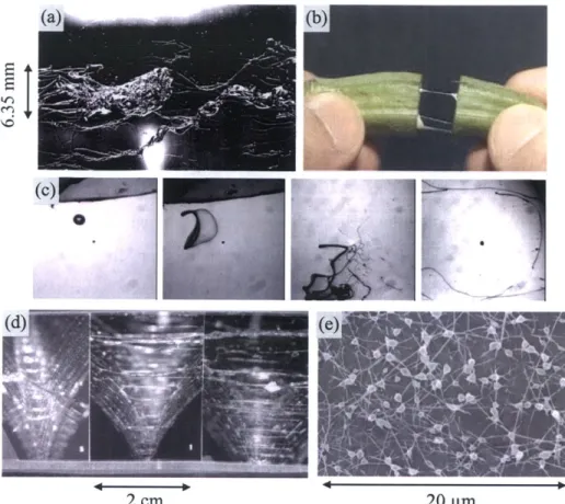
McKinley's review [23] of visco-elasto-capillary thinning of complex fluids gives further applications of extensional rheology. Figure 1-1 shows various break-up phe-nomena of viscoelastic fluids. These include break-up of a high-speed fluid jet contain-ing PEO, threads formcontain-ing from cuttcontain-ing an okra, roll-coatcontain-ing of hydroxyethylcellulose

(HEC), and beads-on-a-string morphology forming in an electro-spinning process.

The significance of extensional rheology in so many areas makes it an interest-ing and important area of study. In this thesis, we want to specifically study the relationship between stress and strain, as well as stress and strain rate, of a fluid in extensional flows.

signifi-(d)(e

2cm

20 prm

Figure 1-1: Examples of break-up phenomena

-

(a) break-up of a high-speed fluid

jet containing PEO, (b) thin threads formed from cutting an ocra, (c) 'bag-break-up'

atomization in a droplet ejected from a nozzle into high-spped cross-stream airflow,

(d) high-speed forward roll-coating of hydroxyethylcellulose (HEC), and (e)

beads-on-a-string morphology forming in an electro-spinning process. Taken with permission

from McKinley [23].

cance because of its interesting properties. Concentrated polymer solutions experience

very little hydrodynamic interactions and excluded volume effects. So in this sense,

dilute solutions actually have more complexity than concentrated solutions.

Concen-trated solutions do, however, have the added complexity of self entanglement [18,19].

Furthermore, the solutions we use in this study are made from a monodisperse

poly-mer. Though we do not compare solutions with varying molecular weights, these

studies can be used to characterize polydisperse solutions. This is done by taking

linear combinations of the monodisperse solutions, of which the polydisperse polymer

distribution is composed, and obtain rheological properties with the appropriate dis-tribution. All of these are useful in characterizing polymers on the basis of molecular weight, stiffness, branching, and hydrodynamic interactions.

To study extensional rheology, we utilize a Filament Stretching Extension Rheometer (FiSER). Our main fluid of interest is a dilute polystyrene in oligameric styrene sol-vent. We will first cover some literature in chapter 2, where we discuss the basics of filament stretching. We will cover the stress and strain tensors specific to filament stretching. We then introduce the kinetic theories that will be used to model the visco-elastic response of the polymer in an elongational flow. In chapter 3, we discuss filament stretching from the view of an experimentalist. We give the details of the hardware that is used in the FiSER. We then go over the different types of filament stretching experiments. In chapter 4, we focus on the motion control of the FiSER. Previous control methods will be reviewed, as well as methods that were considered. We then introduce the Euler method that was used to achieve a constant true strain rate stretching experiment. The stability of this method motivates modifications to algorithm, which leads us to the least squares approximation method.

We present the rheological results in chapter 5, both shear and extensional. We compare the results with theory, again both in shear and extensional. We discuss the agreement and disagreement between the model and experimental data, and give conjectures to the differences. In chapter 6, we give results for stretch-to-break (STB) experiments. These experiments were done with a Newtonian fluid, styrene oil, as well as a weakly elastic fluid, STP@ motor oil. We finally make concluding remarks in chapter 7.

Chapter 2

Literature Review

This chapter provides the theoretical background for extensional flows. We define flow field and geometries that are used. We introduce the polymer science used to model the fluid of interest. Finally, we define the dimensional numbers to show the compe-tition between various effects present in the flow. For an introduction to elongational

flows, with interesting historical notes on the early explorations and developments

of extensional viscosities and other related material properties, see Petrie's book,

Elongational Flows [30].

2.1

Elongational Flow

z

r

Figure 2-1: A fluid sample, simplified as a cylindrical body, being stretched uniax-ially.

In our filament stretching experiments, we first consider a simplified version of the fluid kinematics where the flow geometry can be modelled as a cylinder being stretched in the axial direction. See figure 2-1. As it stretches in the z-axis, the cylinder gets thinner in the r-axis, or x- and y-axes. We can represent the velocity gradient of this flow as:

dvx dx

,V dvy_dx

dvz dx

For an elongation, or extensional, flow, the

dvX dvx dy dz dvy dvy dy dz dvz dvz dy dz /

velocity field is given by:

(2.1) (2.2a) (2.2b) (2.2c) 1 Vx = -- EX 2 1 vy = -- y 2 V2 = z

where is the strain rate, which we will velocity gradient is then:

Vv=

formally define in section 2.2.1. The resulting

_1* 0 0 0 01 0 0 0 (2.3)

The velocity gradient of an extensional flow is purely diagonal, meaning that the flow is shear-free. In the case of filament stretching, where there is axial symmetry,

we can easily represent the velocity field and gradient in cylindrical coordinates: 1. Vr = - r (2.4a) 2 VO = 0 (2.4b)

VZ

= EZ

(2.4c)

As before, we can combine these velocities and represent them as a velocity

gra-dient: dv, 1 dvr, dv 1 0 0 dr r d9 r dz 2 1Vv = _dr _ 1" VO + ' _{r dO r dz} V_ - 0 ₂ 0 ( 2.5) dv, 1 dvz dv0 dr r d9 dz

The strain rate tensor then becomes:

-0 0

=Vv + VvT= 0 -i

0

(2.6)

0 0 2

All of these equations are only valid for purely uniaxial stretching, where we can

consider the fluid sample as a perfect cylinder. In reality, the fluid will not always

deform in such a manner. For short times, t - 0, the velocity field is governed by

lubrication theory. This means that the strain rates in the axial and radial direction will be different from that as given in equation 2.6, and will continue to change until the fluid begins to experience uniaxial stretching.

2.2

Mechanics

Before we can start discussing polymer physics, we need to define some of the geome-tries used in filament stretching experiments. We first establish the important dimen-sions in a generalized stretching experiment. We then show which measurements can

be made, and the material properties that can be calculated from these measurements.

2.2.1

Kinematics

Figure 2-2 shows a very general setup in a filament stretching experiment. The two important length scales are the plate separation, L, and mid-plane diameter, D. The subscript 0 denotes the values of the respective lengths at the beginning of stretch,

i.e., t = 0. As the plates separate, the mid-plane diameter decreases. From the time

evolution of these two lengths, we can define two strain rates - the radial (true) strain rate and the axial (nominal) strain rate:

ldL EL - (2.7a) L dt 2 dDmid D

Dmid dt

(2.7)

L(t) D~t) LO D

Figure 2-2: The endplate separation, L, and mid-plane diameter, D, of a fluid

sample being stretched.

Once we have the strain rates, we can integrate them over time to get the total strains, or what is often called Hencky strain.

it

D

0 ED Ddt

2 in

(2.8a)

JO

Dmid

L

EL = L

n

(2.8b)

fo LO

The Hencky strain in the axial direction takes the same form as the typical true strain defined in traditional solid mechanics. The radial strain is slightly different in that the initial diameter is in the numerator of the logarithmic function. This is because the radius decreases throughout the course of the stretching experiment, but we want the strain to be positive. The factor of 2 is present so that when the flow approaches the uniform elongational flow (UEF) limit, i.e., a cylinder being stretched, the two strain rates are equal.

We can imagine two limits of the filament stretching kinematics. For the early parts of stretching, i.e., small strains, the polymer has not been stretched enough to have any impact on the fluid deformation, so the flow can be considered to be a reverse squeeze flow with the solvent as the fluid. This comes from lubrication theory performed with Newtonian fluid mechanics since the solvent is Newtonian. At larger strains, strain-hardening changes the way the fluid deforms. The deformation is very close to being an uniform elongation flow. The fluid far away from the endplates can be treated and modelled as a one-dimensional flow, as the axial velocity becomes fairly independent of the radial distance [37,36]. Thus, we have a relationship between the two strain rates for our two limits:

3

lubrication: D =-L (2.9a)

2

UEF :D =L (2.9b)

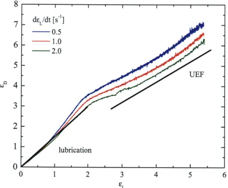
From the two strains, we can construct a master curve. The master curve shows the relationship between the radial (true) strain and the axial (nominal) strain. Fig-ure 2-3 shows a master curve for some typical filament stretching experiments. We

8

7

6

5

WO 4

3

2

1

0

0

1 2 3 4 5 6 EL

Figure 2-3: _{The master curve for a filament stretching experiment.}

see that the master curve depends very much on strain rate. For lower rates, the fluid breaks "faster," i.e., the amount of axial strain necessary to reach a certain radial strain is lower. For the rates shown, the master curve follows the limit given by

lubri-cation theory for strains up to EL - 1.5. It starts to follow the uniform elongational

flow limit at around EL - 3.5.

2.2.2

Dynamics

We now consider the dynamics of stress tensor:

6=

p+ T

a fluid sample being stretched. We first define the

C

p + Trr

0

0 0 p + 7-0 0 0 p + Tzz

)

(2.10)

dEL/dt [s-'] 0.5 - 1.0 2.0 UEF. -

lubrication-ir is stress from the hydrostatic pressure. The fluid stress is purely diagonal because the flow is shear-free. We can avoid dealing with stress associated with the hydrostatic pressure by taking the normal stress difference:

(7zz - 7rr) = (zz - Frr) (2.11) The force balance that allows us to determine the normal stress difference will be given later in section 3.2. From here, we can define the extensional viscosity:

KTzz

- Trr)= E (2.12)

The extensional viscosity is the material property we are after in our study. We would like to measure the steady state value as well as the transient behavior of extensional viscosity. For more in-depth discussions of material properties, see [43] and [26].

2.3

Kinetic Theory of Visco-elastic fluids

Up until now, we have only defined values - geometrically, kinematically, and dynam-ically - that hold for all fluids in extensional flow. We now consider the effects of a polymer chain in a Newtonian solvent. A good overview of the kinetic theory of polymer solutions can be found in Larson's review of dilute polymer solutions [19].

2.3.1

Coarse Graining

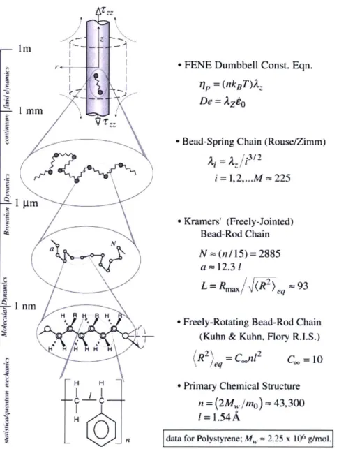
When considering a long polymer chain, we can not possibly look at every single carbon and hydrogen atom. If we take each carbon-carbon chain to represent a freely rotating link, we can then simplify segments of the chain into a link of the Kramer bead-rod chain. We can then further simplify each bead-rod chain into segments of a bead-spring chain. See figure 2-4. In each simplification, called coarse-graining, we reduce the level of complexity of the polymer chain. This is important if we want to simulate polymer behavior during various deformations. The goal is to pick

the appropriate amount of coarse-graining that will give the best results while being simple (computationally inexpensive) enough to compute on a personal computer.

2.3.2

Bead-rod and Bead-spring Models

As shown in figure 2-4, we can represent a freely-rotating chain of molecules as a rod in the bead-rod model. These rods, each representing a Kuhn step, are freely-jointed and follow a conformation that is governed by random walks. The number of rods in a bead-rod model grows with the molecular weight. Current computational capabilities can only handle polymers with a few hundred rods. The computation is expensive not only because of the large number of rods, but also because the time steps required is very small, as the rods move very rapidly. For the polystyrene we use, which has a molecular weight of M, ~ 2.25 x 106 g/mol, the number of rods in the bead-rod model exceeds 1000, making the computational costs too high. Therefore, we coarse-grain multiple bead-rod sections into a spring, resulting in the bead-spring chain.

In the bead-spring model, the spring represents entropic elasticity. This is the effective spring force that is pulling the two ends of the subchain (a chain of N, rods) as the rods are in motion. The beads provide the viscous drag from the solvent on the polymer chains. Since the beads are of a constant radius, the viscous drag will remain constant. To account for the change in viscous drag as polymer chains are stretched and become oriented differently, the springs can be made non-linear to compensate for such changes.

Other forces to consider are hydrodynamic interactions (HI), excluded volume (EV) interactions, Brownian forces, internal viscosity (IV), and self-entanglement

(SE). Hydrodynamic interactions arise when polymer chains influence each other or

itself as they are deformed. In the case of our solutions, which are very dilute, HI comes from polymer chains interacting with itself.

Im -~I I mm

pm

nmn H 8 H

c-c-H H I H

o

n

* FENE Dumbbell Const. Eqn.

p = (nkBT)L

De = Azo

- Bead-Spring Chain (Rouse/Zimm)

12.M 225 * Kramers' (Freely-Jointed) Bead-Rod Chain N (n/15)= 2885

a

12.31 L Rmax/ (I2) 93

- Freely-Rotating Bead-Rod Chain (Kuhn & Kuhn, Flory R.I.S.) R 2\= _/ Cnl2

eq C. =10

* Primary Chemical Structure

n =(2M,,/mo)- 43,300

1=1.54A

data for Polystyrene; MW = 2.25 x 106 g/mol.1

Figure 2-4: The various levels of coarse-graining in polystyrene with molecular weight M, ~ 2.25 x 106 g/mol. Taken from [26].

x

-I

2.3.3

Rouse Model

To ensure that we have chosen the right level of coarse-graining, we check the relax-ation times that the bead-spring chains experience. Since there can be a spectrum times, we notate them as Ai, where the index i indicates the mode number. We first introduce the Rouse model as the simplest bead-spring model. It neglects both HI and EV and uses Hookean springs.

We take the viscous drag on the bead as given by Stoke's flow, where the drag coefficient, (, is given by ( = 67r?7a. Here, , is the solvent viscosity and a is the bead radius. The total drag of the coil is then cOI = (N. Skipping the details of

derivation, we can represent the relaxation times of the ith mode as:

(coil

(R

2 ₎

0

1

A i ~OC- (2.13)

67r2kBTi2 j2

The longest relaxation time has been show experimentally to be related to the intrinsic

viscosity,

[7],

by:

Alongest,R

SNAkB

_(2.14)

where S is a factor representing the distribution of relaxation times.

S = (2.15)

A,

For the Rouse model, i.e., equation 2.13, Si =,7r2/6 = 1.645. The relaxation strength, G, is the same for all modes, i.e., Gi = G, and is given by:

CNAkBT (.6

Gi = G = nkBT = (2.16)

Mo

,

_{Gi (Aiw)}

2

_cNAkBT

N

(A

)

2

1 + (Aw)

2 MW

1 + (Aw)

2 G"()=CNAkBT N~

G1 (C) =

N2 (2.17b)

0

_{1+ (Aiw)}

2.3.4

Zimm model

The Zimm model takes the Rouse model and includes hydrodynamic interactions. As opposed to equation 2.13, where the the relaxation time of the ith mode scales with 1/i 2, the relaxation times are now given by:

A1

AZ = _(2.18)

with the longest relaxation time now given by:

Alongest,z = 1

[

(2.19)

(3v) NAkBT

( is the Riemann zeta function, given by:

001

*

(3v)

=

1

(2.20)

i=1 u is given by:

-1.4 (h*)0.7

_(2.21)

h* is a parameter that represents the degree of hydrodynamic interaction, with h*

0.25 for a theta solvent.1 Taking the value of h* for a theta solvent, we get that the relaxation times scales as Ai

oc

1/il.5 25_.2 _{From this, we can again express the storage}

and loss moduli as a sum of relaxation times and strength. The expression is very

lh* ~ 0.25 was the "special" value that Bird et al. noted in [7]. It is calculated to be h* = 0.267 for the Zimm model using the Flory-Fox parameter for theta solvents [19].

2

similar to equation 2.17, but with some additional terms as the mode number i is more involved in the summation:

-cNAkT Nm z0

G'

= (Aw)2

(2.22a)

1= -cNAkT N__Az_______

(2.22b)

MW i2(2+o)

+ (Azw)

2

In general, experimental data for linear viscoelastic material functions, G' and G", have good agreement with the Zimm theory when the solution is dilute. See section

5.2.1 for comparison of the Zimm theory with experimental data.

2.4

FENE Models

Rheological behavior is often modeled with the FENE-P (Peterlin approximation) dumbbell. This model falls in the most coarse-grained level in figure 2-4. This model, however, does not capture the spectrum of relaxation times that is found in polymeric solutions. The FENE-P chain model can be used to capture the contributions from other relaxation times, but at a heavy cost because of the large number of coupled equations. To model a FENE-P chain with N modes, the number of equations scales with N2_{.Wedgewood [51] proposed the FENE-PM model that uses decoupled} equa-tions. It produces rheological behaviors similar to the FENE-P chain, but at a much lower cost. The calculations required only scale with N. In the following sections, we take a look at how adding more modes to the FENE-PM model affects the stresses, and hence extensional viscosity, in elongational flows. We also try to determine how many modes is required to get a "good" approximation for the stress contribution from the polymer.

2.4.1

FENE-PM

Entov and Hinch study a FENE model with multiple modes in [14], with each mode experiencing a deformation Ai (t). In elongational flow, axial symmetry allows the deformation to be broken down into A, (t) and A,,,i (t). These deformations behave according to:

A' = 2 A' -

1

(fA

- 1) (2.23a)

A?

=

- A

- 1

(fA. - 1)

(2.23b)

where is the strain rate, Ai is the relaxation time of the ith mode. We saw in equation 2.18 that the relaxation time spectrum of the Zimm model scales as A c 4,

with o- being a measure of hydrodynamic interactions. Finally,

f

is a FENE factor determined by:

fN

_(2.24)

2-

A i

A

i=1

L2 is the measure of finite extensibility of the modes, which is the same for all modes.3 This allows us to compute the stress as:

N

p= (nkBT) f Azz'i - A,i) (2.25)

The p subscript denotes stress from the polymer. Total stress can then be calcu-lated from r =Tr + T8, whereT, = 3r7j, is the stress contribution from the solvent.

2.4.2

FENE-PM Simulations

With the equations in 2.23, the deformation can be solved with Matlab's ODE solver. For the following simulations, the material properties used are that of PS025, with

3

1000

IA.

SIA.

e \

_rr,1

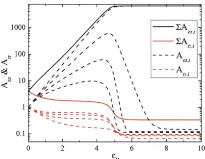
100 --- A. N ZZ,1 rr,1 1 0. 1 -0 2 4 6 8 10 ED

Figure 2-5: FENE-PM for a strain rate of = _{1 s-1. The deformation components,}

Azz,i and A,,,j, for each mode (four total), as well as the sum of all the modes.

longest relaxation time A, = 5.02s, performed at a temperature of T = 250C. Other

relevant properties can be found in table 5.1.

Figure 2-5 shows FENE-PM with four modes under a strain rate of e = 1 s-1

The deformation components Azz,i and A,,,i are plotted for each mode, as well as the sum of all the modes. The first mode sets the steady state value. Subsequent

modes add negligible amounts to the steady state value. From the second mode and onwards, the only contribution is towards the transient response.

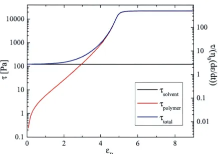
Figure 2-6 shows the polymer stress, rp, for the same strain rate with increasing number of modes. As the figure shows, the addition of each mode has a less and less effect. By the fourth or fifth mode, the stress is very close to what seems like a converging curve. Figure 2-7 shows the total stress, which is the sum of the polymer and solvent stresses.

As expected, Az,, grows to some value, then becomes limited by the FENE pa-rameter,

f,

as the polymer reaches its maximum extension. The first mode reaches a steady state while the others drop. At the first mode, the FENE parameter is just

10000 1000 Nd

:De

100

1

: 5.0225

2 :

1.6683

10

3 : 0.8755

4 : 0.5541

5 : 0.3886

6 : 0.2908

7 : 0.2276

0.1 1 2 3 4 5 6 7 8 9 SD

Figure 2-6: The effect of changing the number of modes used in the FENE-PM

model on the total polymer stress. The strain rate is = 1 s-1. Each line represents

the total polymer stress with the corresponding number of modes that was used.

Additional modes increase the total polymer stress.

10000 1000 100 10 1 0.1 0 2 4 6 8 100 10 0.1 0.01

Figure 2-7: Total fluid stress, as predicted by FENE-PM. Both solvent

contribute to the total stress. The strain rate is

=

1 s-1.

and polymer

solvent

polymer total

at the right size that keeps A,, at the finite length. However, because the FENE parameter is the same for all modes, it actually reduces A,, for the other modes. On the other hand, Arr,i decreases to some steady value.

It is helpful to find a way to determine how many modes are sufficient to model the transient response. We refer to studies on elongational flow with varying De numbers (in the case with no finite extensibility). At high De numbers (De > 1),

the polymer is pulled so fast that it does not have time to relax. As a result, the stress increases exponentially. At De = 1, the stress increases at the same rate as

the area is decreasing, so the force reaches a constant. For j < De < 1, the area decreases faster than the stress, so the resulting force experiences a maximum. The stress still increases exponentially, but not as rapidly as before. At De = ,_{2' the flow} is stretching the polymer just at the rate so that that polymer increases only linearly. At De < , the polymer has time to relax. The flow keeps the polymer stretched at a finite length so that the stress reaches a constant.

The analysis above can be used with FENE-PM models. Each mode will have a slightly different De number, as the relaxation times are different for each mode.

De decreases with each mode. Instead of increasing forever, the stress now has

a maximum limit because the polymers can only be stretched to a finite length. Polymers experiencing De > j will give significantly higher stress contributions than

1

polymers experiencing De <

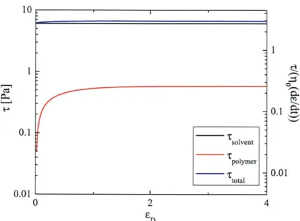
To demonstrate the effects of varying De numbers, figure 2-8 shows a polymer experiencing a strain rate such that the largest De number is less than 1. Note that the stress contribution from the polymer is so low that is dominated by the solvent contribution.

Conversely, if the De is high, then the number of modes needed is increased. Figure below shows a strain rate of 5 s-1, so that the longest relaxation time is A = 25.1 s. The De number does not decrease below I until the 14th mode. As a result, each₂ mode show actually adds a significant amount to the total transient stress response

-i.e., the two outer-most curves.

10 -1 1-0.1 0.1 solvent polymer S.01 total 0.01 0 2 4 E D

Figure 2-8: Total fluid stress resulting from a stretching experiment with a low strain

rate. Here, the strain rate is = 0.05 s-1, giving a Deborah number of De = 0.25.

The solvent stress dominates the polymer stress.

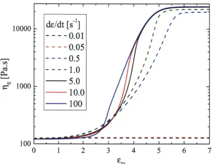
define this in greater detail in the next chapter. Figure 2-9 shows the transient

extensional viscosity for a series of strain rates ranging from e

=

0.1

-

100 s-1.

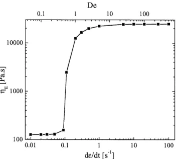
Figure 2-10 shows the steady state extensional viscosity as a function of strain rates

or Deborah number, De. As mentioned above, the extensional viscosity is dominated

by the solvent stresses,

T

E

=

3

77, for low De flows. The polymer stresses do not

contribute until De approaches 1. Above the critical

1

_{value, the extensional viscosity}

2 2

reaches a limiting value set by the length of the polymer chains.

2.4.3

Comments on FENE-PM

In section 2.4.1, we introduced the FENE-PM model. The FENE-PM is in essence

a Rouse chain whose linear springs has been replaced by a FENE springs. Gupta et

al. [16] measured the extensional viscosity of dilute polystyrene solutions with varying

strain rates. His studies showed the results in comparison with FENE-PM and also

FENE-P with the Zimm relaxation spectrum (obtained from shear rheological data).

10000 dE/dt [s , ---- 0.01

- - -- 0.05I

- - -- 0.5

10005 10.0

100

100 - I I I -0 1 2 3 4 5 6 7 ED

Figure 2-9: Extensional viscosity as predicted by FENE-PM, for a range of strain

rates. For low rates, the Deborah number is sufficiently low such that the extensional viscosity is solely determined by the solvent, resulting in a flat line.

of extensional viscosity. The stretching causes the drag on the chains to behave more like a Rouse chain, i.e., it experiences very little hydrodynamic interactions.

2.5

Dimensionless Groups

To measure the fluid stresses, we use a force transducer as the bottom endplate. The specifications of this force transducer will be given in section 3.1.3. There are many forces that contribute to the total force being measured. A detailed force balance will be discussed in detail in section 3.2. Besides the forces that come from the fluid stress, we also need to consider viscous, inertial, gravitational, and surface tension effects. To get a get a good sense of the various degrees of magnitudes, it is useful to define dimensionless numbers to compare the different contributions.

The Reynolds number, Re, is the ratio of inertial to viscous effects. A low Re means that we can neglect the inertial

10 100

0.01 0.1 10 100

de/dt [s1]

Figure 2-10: Steady state extensional viscosity, as predicted by FENE-PM, as a function of strain rate. The x-axis can be represented as strain rate, bottom axis, or Deborah number, top axis. The jump from solvent dominated stresses to polymer dominated stresses occurs at De = .

Re

= inertia _

p

L2

viscous effects o7 =

(2.26)

The Bond number, Bo, is the ratio of gravitational to surface tension effects. A low Bo tells us that we can neglect gravitational effects.

gravity pgD

Bo =surface tension 40-

(2.27)

The capillary number, Ca, is the ratio of viscous to surface tension effects.

viscous effects _ ro0Do

Ca= . =2.25k

surface tension (2.28)

The ratio of the Bond number to the Capillary number represents the ratio of gravitational to viscous effects.

Bo gravity Ca viscous effects pgDO 0.36 = = 0.1 De 10000 1000 100 U, U

* I

U u-u-rn-.--(2.29) I

U-Finally, the Deborah number, De, is the ratio of the material time scale to the experimental time scale.

material time scale

De =-=A = 5 (2.30)

experimental time scale

The material time scale used in our expression is the relaxation time, A, of the polymer solution. The experimental time scale has to do with how fast we are exciting the polymers in the solution, namely the strain rate. As De -- 0, i.e., the imposed

flow is so slow that the polymers are never excited, we reach the Newtonian fluid limit. As De >> 1, we reach the elastic solid limit.

Chapter 3

Filament Stretching

There are different ways to study the extensional rheology of liquids. We will first go over the instrumentation of the experiment, detailing the hardware components that are used in stretching the fluids and measuring the quantities necessary for extensional rheology. We will quickly review the kinematics that was discussed in section 2.2.1 and show how that affects the various stretching experiments.

3.1

Hardware

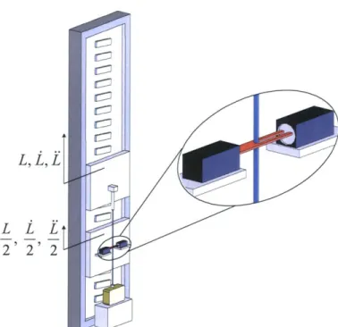
The filament stretching extension rheometer (FiSER) used in our study consists of a DC linear motor, a laser micrometer, and a force transducer. A schematic of the filament stretching extensional rheometer (FiSER) is shown in figure 3-1. A summary of the hardware specifications is given in table 3.1. We now discuss each component in detail.

3.1.1

Linear Motor

The linear motor, made by NorMag (Northern Magnetics, Inc.,1 model EPS-1200), is capable of reaching extensions of 2 m and speeds of 5 m/s. There are two motors on the stage. The top motor carries the top endplate, which in turn stretches the fluid.

L

2'

L

2

Figure 3-1: Schematic of

The bottom motor carries the laser micrometer, which measures the diameter of the

fluid sample. The bottom endplate is the force transducer, which stays stationary.

The laser micrometers always stays at the half-way point between the top and bottom

endplates. Thus, the bottom motor will always travel at half the position, velocity,

and acceleration as the top motor. This allows us to measure the mid-plane diameter

of the fluid sample.

The motors are driven by the Delta Tau Programmable Multi-Axis Controller

(PMAC). The signals from the PMAC are sent through two amplifiers (Glentek

SMA8315-1A-1), which then feed the amplified signals and power to the motors.

Variables and programs are downloaded from and uploaded to a personal computer

(PC, Dell Dimension 8200) through the Delta Tau software interface (PeWin 32 Pro)

via a RS-232 (serial port) connection. Force and diameter measurements are made

through the Delta Tau 16-bit A/D DAQ accessory board (ACC-28B). While the

mo-tion programs are running, all calculamo-tions and communicamo-tion are done within the

PMAC and the motors, and not involving the computer (PC). The PC is only used

the filament stretching extensional rheometer (FiSER).

L , L,L

Table 3.1: FiSER hardware specifications. Motion Lmax 1.5 m ALmin,controllable 150 pm ALmin,observable 1 Am SVmax 2 m/s Diameter Measurement Dmax 9 mm Dmin 50 pm ADmin* 10 pIm Force Measurement Fmax

I_0

g

AFmin 0.01

g

* Refers to resolution, which is different from the smallest measureable diameter,

Dmin-to write the programs, send the programs Dmin-to the PMAC before an experiment, and retrieve the data from the DAQ board after the experiment.

Motion programs are written in a proprietary language specific to Delta Tau con-trollers. The Delta Tau PMAC runs on an internal clock with 447 pus cycle time. Data can be captured at time intervals that are multiples of this cycle time.

There have been other filament stretching rheometers built with different linear motors. Linear motors have different specifications based on manufacturer and model. Furthermore, linear motors are usually paired with specific controllers,2 and different controllers have different capabilities in terms of calculating trajectories for motion blending. For a list and comparison of some of the other extensional rheometers, see

[2].

3.1.2

Laser Micrometer

The laser micrometers are made by Omron (model ZL4A). It is capable of measuring diameters down to 50 pm with 5 pm resolution and has a response time of 0.5 ms. Figure 3-2 shows a typical calibration of the laser micrometers. The data points are acquired with various optical fibers and plastic rods, to simulate the transparency of

the fluid samples.3 The minimum and maximum voltages are 1 and 5 V respectively. 5 V = -0.3208D + 4.9895 2 R 20.9998 > 4-3 --0 1 2 3 4 5 6 7 8 Diameter [mm]

Figure 3-2: Calibration of the Omron laser micrometers.

3.1.3

Force Transducer

The force transducers are made by Futek (Q07512). It is used in conjunction with an amplifier (Futek JM3). The transducer can measure forces of ±10 kdynes (i.e., 10 kdyne in both tension and compression), and has a response time of 50 ms. Figure 3-3 shows a typical force calibration, done with Ohaus@ weights.

We need to determine the dynamics of the force transducer before we can use it to calculate the stresses in the fluid sample. The transducer outputs a voltage to the data acquisition system (DAQ), and the values from the DAQ is then translated to a force measurement. There is complexity introduced by the dynamics, which tells us how the input relates to the output. We analyze the dynamics by creating a Bode plot of output response of the transducer. We excite the transducer at various frequencies

by mounting a magnet on the transducer and holding it under an electromagnet,

which is controlled with a lock-in amplifier (EG&G 7260). We can then measure the

3

For opaque objects, the calibration changes noticeably, but still retains the linear behavior.

'

0 V =-1.OOM - 0.4358 -1 ₂ -2 -3 ---4 -4 6 --7 -8 ---1 0 1 2 3 4 5 6 7 8 Mass [g]

Figure 3-3: Calibration of the Futek force transducer. Ohaus weights were used

to calibrate the transducer in compression. The linearity is preserved with forces in tension (results not shown here).

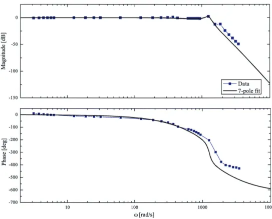
magnitude and phase response of the transducer. From these data, we generate a Bode plot, as shown in figure 3-4.

Once we have a Bode plot, we can try to model it to estimate what a typical response would be. This is done by fitting a linear system of poles and zeros that would result in a similar Bode plot. For the Bode plot given in figure 3-4, we approximated the system to have seven poles. Given these poles, we can simulate a step response of the system. Figure 3-5 shows a step response of the transducer along with the model prediction of the 7-pole system. To simulate a step input experimentally, a weight was placed on the transducer, and pulled off with a string. There is a bit of discrepancy in the initial responses. This is due to the human error introduced as the weight is pulled off manually. The important characteristic is the slope of the curve

- a measure of the rise time4 _{- as it rises from initial to final values.}

The Bode plot of the transducer response tells us that for strain rates of up

4

Rise time is typically defined as the amount of time needed for a signal to change from a specified low value to a specified high value in response to a step input. The specified low and high values are typically 10% and 90%, respectively.

0 -50 -100 -150 0 -100 -200 -300 A -400 -500 -600 -700 10 100 1000 10000 o [rad/s]

Figure 3-4: Bode plot of the Futek force transducer. The blue points are the

data collected by inputting a sinusoidal signal with the EG&G lock-in amplifier and comparing it with the output from the transducer. The black line is the 7-pole linear system that was fit to the data.

to = 1260 s--1, the transducer will theoretically output the force input exactly.

Since the maximum strain rates that the fluid samples are subjected to are orders of magnitudes smaller, we can safely use the raw voltage as a good estimation of the force measurement without having to de-convolute the signal. This is different from the case as presented in Anna's studies

[2].

The force transducer used in Anna's studies had a drop-off frequency of about 126 s-1, about an order of magnitude lower. This means that the transducer's voltage output can lag by as much as 10 ms, depending on the strain rates.

Figure 3-6 shows typical force measurements from two different experiments. Two different rates are shown, the higher rate experiment ends more quickly because the

---e-Data

1.2 I I * I * I 1.0 0.8 o 0.6 0.4 - -_{-2g step} -*-5g step

0.2 _{linear system fit}

0.0

-0.2

-0.02 0.00 0.02 0.04 0.06

time [s]

Figure 3-5: Step responses of the force transducer with two different steps. The

forces have been normalized to be compared with the step simulation done in MatLab.

motors reach the maximum height faster. The force transducer is set close to zero voltage at initial times. Here, positive force corresponds to the transducer feeling a force in tension. As the fluid is stretched, the force "jumps" up to some higher value. The amount of time it takes for the transducer to jump to this higher value is related to the response time of the transducer. It then starts to drop just as a Newtonian fluid would. Then strain-hardening causes the force readings to rise, as the polymers are being stretched. The force readings are more pronounced in the higher rate experiment.

The Futek force transducer experiences noise electrically from the surrounding as well as vibrations from the motor motions. Figure 3-7 shows noise stemming from various sources. The reference reading is taken with all electrical components - motors, amplifiers - off. The data show noise can result from the electrical and mechanical noise. The electrical noise, which mainly come from the amplifiers, are significantly

4 2 --- 3s_ -* - -~ -2 -*3s -2 0 2 4 6 t (s)

Figure 3-6: Typical force readings from a filament stretching experiment.

less than the mechanical noise, which comes from the vibration of the motors. Keep in mind that even when the motors are being asked to stay still, there are still small oscillations in position. This is because the motors are mounted vertically, and so force is constantly being generated to counter gravity.

3.2

Force Balance

To determine the forces that are acting on the fluid sample, we consider half the fluid sample. See figure 3-8. We assume that the fluid sample is symmetric about the mid-plane. The forces acting on this half sample control volume are the forces within the fluid, surface tension, inertia, gravity, and the force transducer, which exerts a force equal and opposite to the force that it measures. The magnitude comparison of these forces, done with dimensional analysis, is covered in section 2.5.

1.4 I * I * I * I 1.2 - -0 all off 1.0 - lamp on M ME 2 amps on 0.8 - m motors on

|

4.

.

M

M

*

motors moving

0.6 -0.6 - -1 g an.m *

*m-0.4

! M!

-0.0 * OF Mpu MEn.* * -0.2 0.0 0.5 1.0 1.5 2.0 2.5 t [s]

Figure 3-7: Noises in force measurements from various sources. For the data with motors moving, the motors were set to move exponentially apart.

FPC

FP

Figure 3-8: Force balance of a fluid sample cut at the midplane. The blue box

marks the control volume.

To determine the fluid stress in the sample, we use the force balance given by Szabo

[45]:

F

[pg6V

0gVO - 1 pVoL

(\zz - Trr) =+ _7R

_R2

₂

1+2irR-+

_7r

_R2

[ _7rR2

_R

-

₂

_7r

_R2

(3.1)

Equation 3.1 shows the various forces acting on the control volume. The term in the ['s, which includes V, applies when the fluid sample is not completely symmetric about the midplane because of sagging effects. This occurs if the strain rates are low and the stress stemming from gravity becomes comparable to the fluid stress. 6V is the extra volume of fluid that has entered the bottom half of the fluid sample. For our calculations, this term will be neglected. This term only becomes important for low strain rates and/or fluids with low viscosities. In such cases of low viscosity, 6V is still often neglected because it is so difficult to measure. Video capture, and most likely video microscopy to get enough resolution to measure the fluid sample geometry accurately, is really the only way to measure the volume of the lower portion of the fluid.

Finally, from equation 2.12, we see that extensional viscosity is related to the fluid stress by (Tzz - Trr) = ?Eieqn : _{Fbal. We can non-dimensionalize the extensional}