HAL Id: halshs-03007904
https://halshs.archives-ouvertes.fr/halshs-03007904
Preprint submitted on 16 Nov 2020
HAL is a multi-disciplinary open access archive for the deposit and dissemination of sci-entific research documents, whether they are pub-lished or not. The documents may come from teaching and research institutions in France or abroad, or from public or private research centers.
L’archive ouverte pluridisciplinaire HAL, est destinée au dépôt et à la diffusion de documents scientifiques de niveau recherche, publiés ou non, émanant des établissements d’enseignement et de recherche français ou étrangers, des laboratoires publics ou privés.
Exchange Rates, Stock Prices, and Stock Market
Uncertainty
Fatemeh Salimi
To cite this version:
Fatemeh Salimi. Exchange Rates, Stock Prices, and Stock Market Uncertainty. 2020. �halshs-03007904�
Working Papers / Documents de travail
WP 2020 - Nr 37
Exchange Rates, Stock Prices, and Stock Market Uncertainty
1
Exchange Rates, Stock Prices, and Stock Market Uncertainty
Fatemeh Salimi Namin
Aix-Marseille University, CNRS, AMSE, France
November 2020
Abstract
While the reference framework for international portfolio choice emphasizes a mean-variance framework, uncovered parity conditions only involve mean stock or bond returns. We propose to augment the empirical specification by using the relative stock market uncertainty of two countries as an extra determinant of their bilateral exchange rate returns. A rise in the relative uncertainty of one stock market will lead capital to flow to the other stock market and generate an appreciation in the currency of the latter. By focusing on the JPY/USD exchange rate returns during the most recent decade (2009-2019) and relying on a nonlinear framework, we provide evidence that the Japanese-US differential stock market uncertainty affects the JPY/USD returns both contemporaneously and with weekly lags. This finding is robust when we control for the stock returns differential and the differential changes in Japanese and US unconventional monetary policy measures.
Key words: exchange rate determination, implied volatility, UEP, flight to safety, flight to quality JEL classification: F31, F32, G15
I am grateful to Eric Girardin for helpful discussions and suggestions. I also would like to thank, without implicating,
Guglielmo Caporale, Yin-Wong Cheung, Christelle Lecourt, Gilles Dufrenot, Kate Phylaktis, Rosnel Sessinou and Zhichao Zhang for their useful comments and suggestions. I also thank Melissa Horn for her help in proofreading. This work was supported by the French National Research Agency Grant ANR-17-EURE-0020.
Address: Maison de l'économie et de la gestion d'Aix, 424 chemin du viaduc, 13080 Aix-en-Provence Email address: Fatemeh.salimi-namin@univ-amu.fr
2
1
Introduction
Modern Portfolio Theory (Markowitz, 1952), in its domestic as well as international versions1 has been based on the first two moments of asset prices, i.e., mean returns and variances. But uncovered parity conditions, specifically Uncovered Interest Parity (UIP) and Uncovered Equity Parity (UEP) (Cappiello and De Santis, 2007; Hau and Rey, 2008, 2006) seem to take a step backward from the mean-variance framework. They assume that capital flows and exchange rate movements are only induced by two countries’ mean (bond or stock) returns differential.2 The role of the second moment as a measure of uncertainty or risk is thus overlooked in investors’ portfolio choice. As a result, despite evidence on the impact of market uncertainty on capital flows (Balakrishnan and Goncalves, 2008; Nier et al., 2014), the relative uncertainty of two countries’ financial markets has not been seriously considered as a driver of exchange rate movements. In this study, we set three objectives. Our primary goal is to evaluate, for the first time, to what extent the relative uncertainty in two countries’ financial markets affects the decision of stock investors to move their investment to the safer/higher-quality market, which in turn appreciates its currency. Consistent with the time-varying effect of uncertainty on financial markets, we pursue this objective in a nonlinear framework. As our second objective, we aim to re-examine the power of relative stock returns in driving exchange rate returns, as suggested by UEP. To do so, we revisit the relationship between the stock returns differential and exchange rate returns in a nonlinear framework. Our third objective is to evaluate the role of the differential between two corresponding countries’ monetary policy stances in driving exchange rate movements. This objective is inspired by UIP, which proposes interest rates differential to be a driving force of exchange rate movements. When the zero-lower bound (ZLB)3 binds in both corresponding countries, and
Unconventional Monetary Policies (UMP) are implemented, the interest rate differential cannot be informative. Instead, we shift our attention toward the differential changes in UMP measures and their nonlinear effect on exchange rate movements.
The main focus of our empirical analysis is on the Japanese yen-US dollar exchange rate (JPY/USD), which is the second most traded currency pair in the global foreign exchange market, after the euro-US dollar (Bank for International Settlements, 2019). We choose this currency pair because it serves as a typical example of the failure of standard variables to drive exchange rate movements. For instance, according to previous studies, the movements of this currency pair do
1 For a review of early literature on international portfolio choice and asset pricing theories refer to Stulz (1995) and
Adler and Dumas (1983).
2 Exchange rate changes are expected to equalize the mean returns from domestic and foreign bonds under Uncovered
Interest Parity (UIP) condition and the mean returns from domestic and foreign stocks under Uncovered Equity Parity condition (Cappiello and De Santis, 2007; Hau and Rey, 2008, 2006).
3 Zero-lower bound binds when the government, in order to stimulate the economy, has used expansionary monetary
policy to the point where the short-term interest rate hits zero. Further stimulating policies should be followed in the form of unconventional monetary policies such as quantitative easing implemented in the US in the aftermath of the global financial crisis in 2008.
3
not comply with UEP (see Hau and Rey (2006) and Curcuru et al. (2014)), and the relationship of the movements of this exchange rate with the UMP measures do not have the expected sign (see Ueda (2012)).
We explore the dynamics of the JPY/USD over the most recent period, after the global financial crisis, from 2009 to 2019. During this period, the two countries experienced episodes of (near-) zero interest rates, and both implemented large-scale UMP. 4 Conducting such an analysis for the
pre-crisis period would require a comparison between two different measures for monetary policy stances of the countries, such as interest rates for the US and reserves growth for Japan, which would be unusual. However, similar measures of the monetary policies of the two countries since 2009 allow us to use a differential UMP variable, facilitating comparison and interpretation. We refrain from including the crisis period during which extreme outliers and noises caused by high volatility may distort estimation results, and because some UMPs were not yet in place.
In this paper, to proxy for stock market uncertainty, we rely on implied volatility indices, such as the VIX index and its counterparts for other stock markets, among the broad range of financial and economic uncertainty measures. We do not intend to thoroughly review these measures here since it has been done by Caporale et al. (2019) and Ferrara et al. (2017). The VIX of the Chicago Board of Exchange is constructed on the basis of the S&P 500 option prices and is a generally accepted proxy for the uncertainty of the US stock market, even being customarily labeled the “fear gauge”. This index has received supportive evidence concerning its explanatory power with respect to various financial markets such as emerging stock markets (Sarwar and Khan, 2019, 2017), commodity-related equities (Badshah et al., 2013; Boscaljon and Clark, 2013; Jubinski and Lipton, 2013; Sari et al., 2011), as well as for capital flows (Balakrishnan and Goncalves, 2008; Nier et al., 2014).
In addition to being reliable uncertainty proxies, we chose implied volatility indices because they suit our purpose in three ways. First, they have a forward-looking nature. Second, they are available at a high frequency. And finally, they represent financial (and not economic) uncertainty. However, such proxies have been criticized in as much as they would not be able to reflect the Knightian uncertainty5 since they do not exclusively reflect uncertainty but include some
forecastable components referred to as risk. Distinguishing between uncertainty and risk components can be essential to establish which one of them is dominantly affected by macroeconomic fundamentals.6 However, such a decomposition is not necessary for the present
study because both components may impact investors’ portfolio choice in a similar way, though
4 Japan has started much earlier in 2001 but reinforced its policies after the global financial crisis.
5 Knight (1921) differentiates uncertainty from risk by defining the former as a situation in which the likelihood of
events happening is not forecastable while the latter relates to a situation in which the probability distribution of events is known.
6 Bekaert et al. (2013) propose an approach to decompose the VIX index into uncertainty and time-varying risk
4
to different extents. Therefore, in this paper, when using these indices, we follow Bloom (2014) in referring to the broad definition of uncertainty, which is a mixture of risk and uncertainty.
In contrast to the implied volatility indices, other proxies of financial uncertainty are at least partially constructed based on historical data and do not fully reflect expectations. For example, the realized volatility of stock markets employed by Chauvet et al. (2015) is a backward-looking proxy. In turn, the variance risk premium proposed by Bollerslev et al. (2009) and employed by Londono and Zhou (2017) and Aloosh (2014) relies on the difference between the realized and implied variances, creating a combination of forward-looking and backward-looking components. Economic policy proxies are usually meant to capture economy-, business- or firm-level uncertainties and are not limited to financial uncertainty. For instance, the most popular economic uncertainty proxy, i.e., the news-based Economic Policy Uncertainty (EPU) index of Baker et al. (2016), reacts more to policy-related events as opposed to the VIX which is highly affected by financial events (Baker et al., 2016). Similar to VIX, EPU has been used in a diverse range of applications, particularly for predicting business cycles (see Caporale et al. (2019)). Similarly, Bachmann et al. (2013)’s empirical business-level proxies are constructed using business climate survey data. A major drawback of economic uncertainty proxies (except econometrically-generated, and thus ex-post ones) is that in contrast to implied volatility indices, they are available neither at high frequencies nor for all countries.
Recently, sophisticated econometrically-driven proxies have been proposed–for instance, by Ferrara et al. (2014) with a conditional volatility model, Jo and Sekkel (2019) with a factor stochastic volatility model, Gilchrist (2014) based on firm-level time-varying equity volatility, and Carriero et al. (2018) thanks to the use of a large VAR model with stochastic error volatility depending on aggregate macroeconomic and financial uncertainty, among many others (refer to Ferrara et al. (2017) and Carriero et al. (2018) for comprehensive list of previously proposed measures). These econometrically-driven proxies are also backward-looking and indicate economic rather than financial uncertainty. Finally, the recursive estimation of expectations by Jurado et al. (2015) and Joëts et al. (2017) help create a forward-looking measure using a sophisticated stochastic volatility model for the unpredictable component of a large set of macroeconomic and financial variables.
This study draws on three strands of literature. First, we draw on the emerging literature that emphasizes the ability of stock markets’ uncertainty to predict exchange rate movements. Intuitively, when high stock market uncertainty or volatility is accompanied by low equity prices, investors fly to safety or quality (Baele et al., 2018).7 Because capital flows connect stock markets
7 Rebalancing portfolios toward safer assets which are less volatile and more liquid such as government bonds, gold,
or safe haven currencies such as the Japanese yen, Swiss franc or the US dollar, following heightened uncertainty and low returns in the market, is known as flight to safety or quality. For theoretical background on flight to safety refer to Vayanos (2004), Caballero and Krishnamurthy (2008) and Brunnermeier and Pedersen (2009) among others.
5
through the foreign exchange market, the movements of capital toward the safer market induce an appreciation of the currency corresponding to the safer market, with more intensity during periods of market stress (Vayanos, 2004). Among the few studies which investigate this relationship, Londono and Zhou (2017) show that the US stock variance risk premium can forecast exchange rate movements. They use the US stock variance premium as a measure of unexpected volatility computed as the difference between the option-implied and the expected realized stock variance. They find that a higher stock variance risk premium indicates a rise in uncertainty in the US stock market, which in turn depreciates the USD.8 In a similar attempt, Aloosh (2014) finds evidence
of the predictability of the returns of the euro, yen, and British pound against the USD by a value-weighted average stock variance risk premium at a one-month horizon.9
A shortcoming of this strand of literature stems from the unilateral view underlying the variance risk premium. This view can result in biased conclusions, specifically in cases when both currencies involved are safe-haven currencies such as the JPY/USD. In such cases, an investor needs an evaluation of the relative uncertainty of the two corresponding countries, which can affect exchange rate movements.10 Therefore, we put forward the use of a simple differential measure,
consistent with the comparative view of an investor to the uncertainty of two stock markets. We call it “differential fear” or the implied volatility (IV) differential. It is defined as the difference between the CBOE’s implied volatility index (VIX) and its Japanese counterpart at the Osaka Securities Exchange, VXJ, calculated based on Nikkei 225 option prices. Besides, we depart from the existing literature by focusing mainly on uncertainty, instead of risk premiums, which involve limitations associated with expected realized variance.
In pursuing the second objective of this study, we draw on the literature on UEP (Cappiello and De Santis, 2007; Hau and Rey, 2008, 2006). This parity condition relies on two underlying mechanisms. The first is that following an outperformance of a foreign over the domestic stock
8 In a different approach, Della Corte et al. (2016) and Londono and Zhou (2017) investigate the role of currency risk
premium in explaining exchange rates. Della Corte et al. (2016) introduce currency volatility risk premium (“the difference between expected future realized volatility and a model-free measure of implied volatility derived from currency option”). They argue that currencies with low implied volatility relative to historical realized volatility have cheap volatility insurance and vice versa. Therefore, investors rebalance their portfolio toward the currencies with cheaper volatility insurance and predictably induce their appreciation. Similarly Londono and Zhou (2017) use global currency variance risk premium (the average of the differences between option-implied and the realized variance of returns of several currencies against the USD) and find that a higher currency variance risk premium signifies a heightened level of global uncertainty and induces an appreciation of the USD as this currency acts as a safe-haven currency.
9 Balakrishnan et al. (2016) blame the lack of attention to the time-varying risk pricing for the failure of traditional
models. Using foreign exchange risk premium (constructed based on interest rate different and Consensus exchange rate forecasts), they show that shocks to the global risk sentiment induce dollar appreciation against major currencies complying with the safe-haven status of the USD and flight-to-safety phenomenon.
10 Looking from a different angle, capital flows, which link different stock markets to the foreign exchange market,
are also influenced by the uncertainty in stock markets. In this regard, Nier et al. (2014) document that during volatile periods, the CBOE’s implied volatility index (VIX) is a major determinant of gross capital flows whereas economic fundamentals prevail during low-volatility periods. Fratzscher (2012) also shows that capital flows are influenced by global shock such as crisis and global liquidity and risk.
6
market, investors repatriate their portfolio to reduce their foreign exchange rate risk. Therefore, capital flows toward the domestic stock market.11 The second mechanism consists of the
depreciation of the foreign against the domestic currency in response to the investment repatriation (selling foreign and buying domestic assets).
Despite the logical and intuitive mechanisms underlying UEP, this parity condition has received mixed empirical support. The most extreme case of rejection is reported by Cenedese et al. (2016), who evaluate UEP using a trading strategy for a sample of 43 countries from 1983 to 2011. In attempts to rationalize the unfavorable evidence on UEP, Kim (2011), Fuertes et al. (2019), and Cho et al. (2016) argue that UEP holds when both corresponding countries are among developed countries. They even suggest that for an emerging economy, the relationship between stock returns differential and exchange rate movements can be the opposite of what is indicated by UEP. Cho et al. (2016) identified that flight to quality during turmoil can be a major driver of exchange rate movements when at least one of the two economies is an emerging one. Along the same lines, Fuertes et al. (2019), find that the divergence from UEP increases in turmoil due to investors’ return-chasing behavior, and suggest that risk pricing is essential in exchange rate determination. While Cenedese et al. (2016) blame systematic equity market risk and global equity volatility risk for the failure of UEP, Kim (2011) argues that significant market risk and government restrictions on capital outflows in emerging markets contribute to this failure. In general, these studies agree that the relevance of UEP depends on investors’ assessment of the relative uncertainty in two markets. Surprisingly, however, neither of these studies considers that relative uncertainty can play a role in the decisions of an international investor, and subsequently affect capital flows and exchange rate movements.
Finally, to investigate the third objective, we draw on the literature on the effects of UMPs (such as forward guidance, large-scale asset purchases, and Quantitative Easing (QE)), implemented by central banks during the (near-)zero interest rate period, on exchange rate dynamics. The existing literature argues that this kind of policy mainly influences asset prices and, subsequently, exchange rates by affecting market expectations through at least four main channels. The first channel is the portfolio-balance channel aimed at boosting demand for riskier assets, following large purchases of specific assets by the central bank, which reduce their supply and lowers the term premium (Gagnon et al., 2011). The second channel is the liquidity channel through which asset prices are affected by the presence of the central bank as a consistent and significant buyer in the market (Gagnon et al., 2011). The last two channels, which are more informational, are the signaling and the confidence channels. The former can induce demand for (the foreign or domestic) higher-yielding assets by informally communicating the commitment of the central bank to keep yields low (Bauer and Rudebusch, 2014). The latter can affect asset prices by providing information to
11 Although, the true incentive behind capital movements following such an outperformance of the foreign over the
domestic market is still open to further research and Curcuru et al. (2014), introduce carry trade or return chasing behaviour of investors as the underlying reason.
7
investors, through easing announcements, on the current and future good health of the economy (Fratzscher et al., 2018).
The existing literature considers that in an open economy framework, the dominant effect of easing policies is a depreciation of the currency of the country implementing it vis-à-vis the high-yielding currencies (Glick and Leduc, 2012; Kenourgios et al., 2015; Neely, 2015; Rosa, 2012; Ueda, 2012). This effect is anticipated because yields are expected to be low for an extended period in the country implementing UMP, inducing capital outflows. However, Ueda (2012) documented that the JPY, differently from other currencies, appreciated against the USD in response to some UMP announcements by the Bank of Japan (BoJ) from 1999 to 2011.
Most of the literature focuses either on cases where only one of the two corresponding countries implements UMP or completely neglects the equally-important effect of the monetary policies of the other country on the exchange rate (Fratzscher et al., 2018). Accordingly, inspired by UIP and consistent with our relative view, we consider whether the differential of the changes of the UMP measures can partially explain exchange rate dynamics.
In addition to the sign of the effect of UMP on exchange rate dynamics, its intensity can also vary over time. For instance, Gagnon et al. (2011) state that the liquidity channel may be functioning more effectively during the first stages of UMP. Fratzscher et al. (2018) claim that the effectiveness of UMP depends on changes in macro-financial uncertainty, i.e., in periods of low macroeconomic uncertainty, the US capital outflows rise following QE announcements. Therefore, nonlinearity is an essential characteristic of such relationships, which has often been neglected in the literature. In this study, we use the nonlinear Markov-switching framework of Hamilton (1989) to fulfill our three objectives. The advantage of this model is that it allows time-varying but recurring relationships between variables where regime changes are endogenously determined (as opposed to the structural break detection of Bai and Perron (2003)). We avoid the use of a nonlinear VAR model or a system of equations.12 In a linear VAR model, the number of parameters grows with
the square of the number of variables included in the model, which exhausts the degrees of freedom very quickly, leading to imprecise estimation of parameters (Krolzig, 2003). This problem can be amplified in a Markov-switching framework, in which all model parameters are allowed to switch. Therefore, to avoid the curse of dimensionality, we prefer to consider a single-equation model.13
We reach three main results. First, the IV differential plays a significant role in explaining exchange rate dynamics. The findings follow our intuition that higher uncertainty in the Japanese relative to the US stock market encourages investors to rebalance their portfolio toward the less risky market and leads to a depreciation of the Japanese yen vis-à-vis the US dollar.
12 For the sake of comparison, a linear VAR model is also estimated and the results are available in Appendix. 13 Using Granger causality tests, we ensure about the lack of a two way causality between the independent variables
8
Second, we find that the stock returns differential is an important driver of the JPY/USD exchange rate movements at a one-week horizon. Following an outperformance of the Japanese over the US stock market, the Japanese yen depreciates against the USD at a one-week horizon. Previous studies never detected this UEP-consistent finding for the JPY/USD, mostly because they rely on samples chosen regardless of the specificities of the two corresponding countries. This effect does not last more than one week, which is in line with the rapid reflection of market participants to events in financial markets.
Third, the differential of the changes in the Japanese and the US UMP measures (reserves growth differential) partially explains the JPY/USD exchange rate movements at one- and two-week horizons. The effect has opposite signs in the two regimes of our model from 2009 to 2019. During the high-volatility regimes of the foreign exchange market, the relationship between the reserves growth differential and the JPY/USD is positive (depreciation of the JPY) in one- and two-week horizons. The depreciation effect is expected inasmuch as more UMP in a country with low-yields finances investments in high-yields countries. However, in the low-volatility regime of the foreign exchange market, the relationship is negative (appreciation of the JPY) at a one-week horizon and changes sign after a week. We conclude that the ultimate effect of a relatively higher increase in the Japanese relative to the US reserves is the depreciation of the JPY against the USD. However, the transitory impact can be affected by the instruments used to implement UMPs.
Our paper contributes to the related strands of literature in several ways. First, the most important contribution of our paper is to put forward a new differential variable as a candidate for the determination of exchange rate dynamics. We underline that not only stock returns differential, but also the differential of stock markets’ uncertainty or the “differential fear” can impact exchange rate returns. Second, we provide evidence of the nonlinearity and time-variability of the relationship between the stock returns differential and exchange rate returns. This nonlinear characteristic is highlighted by the fact that while we provide UEP-consistent evidence for JPY/USD over a recent sample, previous studies never found it over earlier samples. And finally, we stress the importance of having a relative view of the monetary stances, stock returns, or uncertainty levels of the two sides of a currency pair when assessing the movement of an exchange rate. An exclusively unilateral view, forgetting the bilateral nature of an exchange rate, may lead to a misleading conclusion.
The rest of the paper is organized as follows: In section2, we present the data and the modeling strategy we use. In section 3, we provide the results of our empirical investigation concerning the three objectives of this study. Section 4 provides concluding remarks.
2
Data and Methodology 2.1 Data9
of the JPY/USD exchange rate returns from January 2009 to July 2019 obtained from the Pacific Exchange Rate Service. Exchange rate returns computed as:
𝑅, ln
𝑃,
𝑃 , (1)
with l being currency pair and 𝑃, its spot price at time t.
We investigate the power of three differential variables in explaining exchange rate movements. The first is the differential of uncertainty measures of the two countries, which is computed using logarithms of the VXJ and VIX indices. Data on both indices are obtained from Datastream. The IV differential is shown in the lower panel of Figure 1. It is worth mentioning that although the VIX is taken by many as a global uncertainty index, it is, in fact, a composition of both global and US factors (Balakrishnan and Goncalves, 2008). By taking the differential of the VXJ and VIX, we aim for our differential variable to be mostly free from the global factor.
The second variable is the stock returns differential, as suggested by the UEP literature. We compute weekly averages of the differential of the Nikkei 225 and the S&P 500 daily returns as
Diff_SRt = RNIK, t – RS&p500,t with RNIK, t, and RS&p500,t being calculated following Equation (1) (see
the upper panel of Figure 2 for a graph of this variable). We use these two indices as the representatives of the Japanese and the US stock markets, respectively.
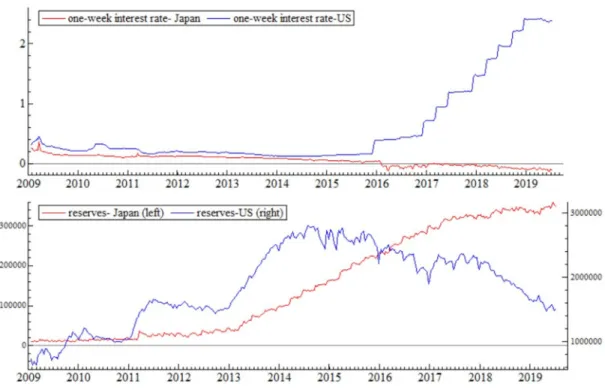
The last variable, as suggested by UIP, should be the interest rate differential. However, as shown in the upper panel of Figure 2, interest rates of both Japan and the US have been almost zero since the beginning of our sample in 2009. While the Japanese short-term interest rate continues to linger around zero, the US short-term interest rate has been rising gradually since late 2015. Therefore, for the whole sample, interest rate differential (as suggested by UIP) cannot be informative in explaining exchange rate movements. Instead, we focus our attention on UMP measures, which can be used as indicators of monetary policy stances of the two countries.
The quantitative easing policy started in late 2008 in the US in the aftermath of the global financial crisis to stimulate the economy. The policy resulted in financial institutions holding excess reserves with the Federal Reserve. The Federal Reserve started tapering policies in 2013, which led to the decrease of these reserves from early 2014 (lower panel of Figure 1). In contrast to the US, the quantitative easing started much earlier in Japan, in March 2001, to trigger the sluggish economy. The BoJ stopped implementing this policy in 2006, but it was resurged after the global financial crisis in late 2008 at a low pace. In October 2010, the Comprehensive Monetary Easing (CME) policy was launched. Later in April 2013, the Japanese UMP was reinforced in the form of a Quantitative and Qualitative Easing policy (QQE), which was followed by a negative interest rate policy in early 2016. All the policies implemented after December 2010 allowed the BoJ to purchase ETFs in addition to government bonds. These policies contributed to an ever-growing
10
expansion of the reserves held at the BoJ and its current account outstanding balance.14
We use the growth rate of the commercial banks’ reserves held with the BoJ and the growth of the excess reserves maintained with the Federal Reserve, which are calculated as (Rl,t ) using Equation
(1) with l being the reserves held with the BoJ or the Federal Reserve and 𝑃, their values at time
t. The differential of growth in reserves is computed as Diff_ΔLRES = RRES(JP) – RRES(US). The
Japanese and the US data are obtained from CEIC and the Board of Governors of the Federal Reserve System at weekly and fortnightly frequencies, respectively. We conduct our analysis at the weekly frequency to be consistent with the rapid responses of financial variables to changes and events. To match the frequency of the US reserves, we use the Litterman method (1983)15 of
temporal disaggregation using money supply (money zero maturity) as the indicator variable. Both the IV differential and stock returns differential include extreme values in March 2011, corresponding to the highest uncertainty in the Japanese stock market at the time of the Tsunami
14 for more details about the Japanese QE, CME and QQE refer to Ueda (2012), Harada and Okimoto (2019) among
others.
15 Litterman’s method of temporal disaggregation for deriving high-frequency from low-frequency time series. This
method is a variant of Chow and Lin (1971) method which interpolates low-frequency series by relating it to a reference high-frequency series based on a regression.
Figure 1 The Japanese and the US stock returns differential (upper panel) and the implied volatility differential of the Japanese and the US stock markets (lower panel)
11
in Japan. Signals of the weakened Chinese manufacturing figures bundled with the tapering news from the US and spikes in the Japanese government yields caused a heightened uncertainty in the Japanese stock market in late May 2013, which in turn lead to high values for both the IV and stock returns differentials. The extreme values of the IV and stock returns differentials in early 2016 correspond to the introduction of negative interest rate policy (on commercial banks’ accounts at the BoJ) in Japan, which was designed to encourage more lending by banks.
Elevated uncertainty in global markets in June 2016 encouraged more purchases of ETFs and the US dollar lending by the BoJ in July 2016. Simultaneously, there were concerns about the deferral of the consumption tax hike in Japan, which contributed to more uncertainty in the Japanese market. In January and February 2018, the fear of an increase in the US interest rates and overdue market corrections caused a sharp fall in major US stock indices and high uncertainty in the US stock market, leading to a negative IV and stock returns differentials. The last extreme value included in our sample corresponds to a negative IV and stock returns differentials when a combination of negative signals contributed to bearish expectations among investors in the US. These negative signals include the tension between the US and China over trade tariffs, slow
Figure 2 One-week interest rates and reserves
Notes: one-week interest rates of Japan and the US in the upper panel and commercial banks’ reserves held with the Japanese and the US central banks in the lower panel (in billions of JPY and millions of USD, respectively).
12 economic growth at the global level, and Brexit.16
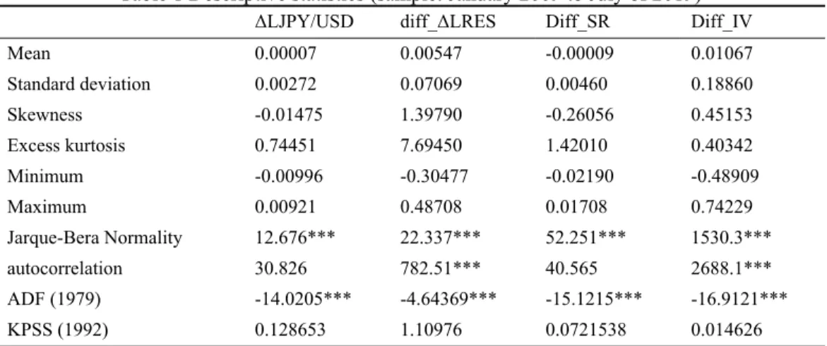
Table 1 shows the descriptive statistics and stationarity results of the exchange rate returns, stock returns differentials, the IV differential, and the reserves growth differential. All variables have non-normal distributions. Besides, the IV differential and the differential of reserves growth suffer from serial autocorrelation. According to the unit-root, ADF (1979), and stationarity, KPSS (1992), tests all variables are stationary.
The use of returns or differenced data may cause a concern, that is, possible long-run relationships between the exchange rate and the levels of explanatory variables are overlooked. Among the three differential variables, the IV differential is computed using the levels of the IV indices and is already stationary. Therefore, a long-run relationship between this variable and the level of the JPY/USD exchange rate is ruled out. The stock returns differential, and the reserves growth differential are computed using first differences of the variables because this approach is intuitively acceptable and theoretically supported. However, to ensure that we do not overlook the long-run aspect of the analysis, we try computing these two differential variables using levels of their constituent components (i.e., logarithms of the stock prices and logarithms of the level of reserves). The results of stationarity and cointegration tests show that the differential of reserves computed using log levels of reserves is stationary and the differential of log stock prices is non-stationary. However, even the latter does not form any long-run relationship with the exchange rate (as reported in Table A 1 in the Appendix).
16 for more details see Arbatli et al. (2017), Le Moign et al. (2018).
Table 1 Descriptive statistics (sample: January 2009 to July of 2019)
ΔLJPY/USD diff_ΔLRES Diff_SR Diff_IV
Mean 0.00007 0.00547 -0.00009 0.01067 Standard deviation 0.00272 0.07069 0.00460 0.18860 Skewness -0.01475 1.39790 -0.26056 0.45153 Excess kurtosis 0.74451 7.69450 1.42010 0.40342 Minimum -0.00996 -0.30477 -0.02190 -0.48909 Maximum 0.00921 0.48708 0.01708 0.74229 Jarque-Bera Normality 12.676*** 22.337*** 52.251*** 1530.3*** autocorrelation 30.826 782.51*** 40.565 2688.1*** ADF (1979) -14.0205*** -4.64369*** -15.1215*** -16.9121*** KPSS (1992) 0.128653 1.10976 0.0721538 0.014626
*** Significant at the 1% level.
ΔLJPY/USD: returns of the Japanese yen vis-à-vis the US dollar, Diff_SR: the differential between the Japanese and the US stock returns (Diff_SRt = RNIK, t – RS&p500,t), diff-IV: the differential between
the logarithms of the VXJ and the VIX (LVXJ-LVIX), diff_ΔLRES: differential of the changes in the reserves held with the BOJ and the Federal Reserve (Diff_ΔLRES = RRES(JP) – RRES(US)).
13
2.2 Methodology
The determinants of exchange rates can vary depending on the economic situation and implemented economic policies, investors’ behavior, and investing technologies, among other factors. For instance, when the interest rates differential is zero or very close to zero, it may not play an essential role in determining the dynamics of exchange rates, leaving room for a temporary effect of other variables. Therefore, it is advisable to use a nonlinear model to capture this time-varying exchange rate dynamics. Accordingly, we use the Markov-switching model of Hamilton (1989), which, in contrast to structural break tests, benefits from the possibility of regime recurrence (Hamilton, 2016).
To analyze the determinants of the JPY/USD exchange rate returns, we use the following general specification:
Δ𝑒 𝛼 𝑠 Δ𝑒 𝛽, 𝑠 𝑑𝑖𝑓𝑓, 𝜎 𝑠 𝜀 (2)
where Δ𝑒 , the JPY/USD exchange rate return, is regressed on its 1 to p lagged values (Δ𝑒 ). The matrix 𝑑𝑖𝑓𝑓, contains the contemporaneous and lagged values of the three differential variables with j indicating stock returns (SR), implied volatility (IV) or reserves growth (ΔLRES), and k the number of lags varying from 1 to q. The error term 𝜀 follows a Gaussian white noise process with covariance matrix Σ.
In this equation, 𝑠 is an unobservable variable that specifies the state at each time. We allow all the parameters in this model to switch state. Therefore, 𝛼 𝑠 s are the state-dependent coefficients of the p autoregressive lags of exchange rate returns. Similarly, 𝛽, 𝑠 s are the state-dependent
coefficients of the stock returns differential, IV differential, and the reserves growth differential. 𝜎 𝑠𝑡 is the state-dependent variance.
The state variable (𝑠 ) follows a first-order Markov chain, implying the dependence of the current value of 𝑠 only on its immediately preceding value. According to our model specification, each observation is designated to a specific state, allowing us to obtain smoothed transition probabilities from one state to the other and the probability of persistence of each state. Estimation of the model parameters is done using the sequential quadratic programming algorithm of Lawrence and Tits (2001) along with a pre-estimation with the Expected Maximization (EM) algorithm of Dempster et al. (1977).
In this empirical analysis, we choose the number of regimes based on statistical tests. To determine the best number of regimes and the best number of lags for the dependent and independent variables, we follow a two-step approach. The first step consists of determining the number of lags to include in Equation (2). To do that, we estimate a vector autoregressive model in a linear
14 framework as follows:
𝑌 Π 𝑌 𝜉 (3)
in which Y is a vector of all our four variables [diff_IV, diff_ΔLRES, diff_SR, ΔLJPY/USD] with
l=1 to 12. We compare the estimated models with 1 to 12 lags using different information criteria,
e.g., the Schwarz (SC), Akaike (AIC), and Hannan and Quinn (HQ) information criteria and we choose the model which yields the lowest value for the information criteria. We use the Granger causality test to ensure the one-way causality from the independent variables to the JPY/USD returns. In the case of a two way-causality, the time t value of the independent variable can be neglected to avoid a simultaneity issue.
A prerequisite to the MS estimation of Equation (2) is to test the outperformance of a Markov-switching model over a linear model. We benefit from the optimal test of Markov-Markov-switching by Carrasco et al. (2014), which only requires the estimation of the Markov-switching model under the null hypothesis of constant parameters. We compute the critical values from 500 iterations for a model that allows switching intercept and variance. Conditional on the rejection of the linear model by this test, we proceed to the second step using the optimal lag suggested by the information criteria from the preceding step.
We allow all the parameters to be regime-dependent and estimate five models with 1 (linear model) to 4 regimes. We compute the Markov-Switching Criterion (MSC), developed by Smith et al. (2006). This criterion is based on the Kullback–Leibler (KL) divergence. As opposed to AIC, SC and HQ, which mislead users to choose an inaccurate number of regimes (Psaradakis and Spagnolo, 2003; Smith et al., 2006), MSC is shown to be efficient across different sample sizes and with noisy data (Smith et al., 2006). This criterion uses full-sample smoothed probabilities in order to balance the fit of the model with its parsimony. The criterion is computed as:
𝑀𝑆𝐶 2𝐿 𝜏̂ 𝜏̂ 𝑆𝜂
𝜏̂ 𝑆𝜂 2 (4)
where L is the log-likelihood of the estimated model, S is the number of regimes, and η is the number of regressors. 𝜏̂ is defined as the sum of smoothed probabilities of being in rth regime
computed using full-sample smoothed probabilities. The model which yields the minimum MSC is chosen as the optimal number of Markov-switching regimes. After selecting the optimal number of lags and regimes, we test whether the linearity of each of the parameters can help improve the fit of the model according to SC.
15
3
Determinants of the JPY/USD Movements
3.1 Markov-switching Model Estimation
Following the first step of our approach, we choose a model with two lags for the dependent and independent variables. Table A 2 in the Appendix shows that all the three criteria choose a model with two lags for the sample from 2009 to 2019.17 According to the Granger causality test results
in Table A 3 in the Appendix, the only variables between which a two-way causality is possible are the exchange rate movements and the stock returns differential. The exchange rate movements can influence the stock returns differential. Therefore, in our nonlinear estimation of Equation (2), we omit the time t value of the stock returns differential and only allow its lagged values in the model as explanatory variables. In the second step, MSC suggests a model with two regimes (Table A 5 in the Appendix). As shown in Table 2, Carrasco et al. (2014)’s test of Markov-switching versus a linear model rejects the null of linearity. Carrasco et al. (2014)’s test results are also confirmed by the MSC, which shows that the outperformance of a linear model is rejected. According to our systematic model comparison using SC, we choose a model in which only four parameters are regime-dependent (Table 3). In this model, the constant term is not significant. Therefore, none of the regimes can be designated to a specific direction of either appreciation or depreciation of the JPY vis-a-vis the USD. The first regime is the dominant and the most persistent (see Table A 6). The variance of the error terms is the parameter that usually governs the regime changes. Therefore, the first and second regimes are the low- and high-volatility regimes, respectively. Apart from the variance of the error terms, only the second autoregressive lag, the second lag of the IV differential, and the first lag of the reserves growth differential are regime-dependent, according to SC.18 The coefficients of the first and second autoregressive lags are
significant with opposite signs, therefore contributing to the JPY/USD appreciation at a one-week horizon and its depreciation at a two-week horizon, respectively.
In accordance with our conjecture, we find a non-switching, positive, and significant relationship between the JPY/USD exchange rate returns and the contemporaneous value of the IV differential during the whole sample. This shows that when volatility is higher in the Japanese stock market in comparison with the US stock market, investors move a part of their portfolio to the safer market (the US market) and induce a depreciation of the Japanese yen vis-à-vis the US dollar and vice versa. This is in line with the findings of Londono and Zhou (2017) and Aloosh (2014). However, it is obtained in a much less complicated framework and taking a two-country relative perspective. This relationship reverses sign in a two-week horizon. In other words, the coefficient of the second
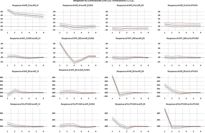
17 For the sake of comparison between the linear and nonlinear estimations (although the models are not identical), we
provide the generalized impulse responses of the VAR estimation in the Appendix (see Figure A 1). The impulse responses show that the exchange rates only react to a shock to the stock returns differential and are not influenced by the shocks to the IV differential and reserves growth differential.
16
lag of the IV differential is significant and negative in both regimes, with a stronger appreciating effect on the exchange rate during the high-volatility (second) regime. This may be a sign that investors move their capital to the market that has already passed an uncertain period, hoping that they can benefit from a “buy the dips” strategy.
The JPY/USD returns have a significantly positive and non-switching relationship with the stock returns differential at a one-week horizon. The positive sign of this coefficient is consistent with UEP, meaning that relatively higher stock returns in Japan lead to a depreciation of the JPY vis-à-vis the USD at a one-week horizon. The coefficient of the second lag is, however, not significant. Therefore, as expected from the fast reactions of investors, the effect of the stock returns differential is short-lived. The UEP-consistent finding at a one-week horizon is unique to this study. The key to this finding is the choice of the sample with regard to the specificities of the two corresponding countries, which was neglected by previous studies.
Finally, the reserves growth differential and the JPY/USD exchange rate returns are not contemporaneously related; however, with one and two weeks of lag, their relationship is significant. The effect with a one-week lag is regime-dependent. During the low-volatility (high-volatility) regime, relatively higher (lower) Japanese reserves growth leads to a stronger (weaker) JPY against the USD. Regardless of how the reserves growth differential affects the exchange rate returns in a one-week horizon, the effect with a 2-week lag contributes completely to a depreciation of the JPY vis-à-vis the USD. The depreciation effect is much more expected in the literature. The appreciation of the JPY against the USD following reinforcement of UMP in Japan has been a source of ambiguity in previous studies such as Ueda (2012) (for a sample from 1999 to 2011).19
One piece of conjecture about the channel through which the reserves growth differential occasionally leads to an appreciation of JPY against the USD is that the Japanese UMP relatively succeeded in guiding investments toward more risky assets inside Japan at a one-week horizon. This could have taken place either by incentivizing investors to rebalance their portfolio toward more risky Japanese assets or by the BoJ’s direct purchases of ETFs since December 2011 under
19 In contrast to the results of the linear VAR model (presented in the Appendix, Figure A 1), the Markov-switching
model shows that the movements of the JPY/USD are also influenced by the IV differential and the reserves growth differential.
Table 2 Linearity vs. Markov-switching test of Carrasco et al. (2014) (sample: 2009/09/26-2019/07/08)
Dependent variable supTS expTS
ΔLJPY/USD 12.689 [0.000] 127.181 [0.000]
Numbers in squared brackets are p-values.
Critical values are computed from 500 iterations for a model with switching mean and variance.
SupTS shows a sup-type test statistic used by Davies (1987), and expTS shows an exponential-type test statistic suggested by Andrews and Ploberger (1994).
17 the CME policy.20
In contrast, the literature enlightens us more about the channel through which the reserves growth differential leads to a depreciation of the JPY vis-à-vis the USD. During the high-volatility periods,
Table 3 Estimated Markov-switching model (sample: 26/09/2009-08/07/2019)
Regime 1 Regime 2 Constant 0.0001 (0.0001) ΔLJPY/USD (-1) -0.1191** (0.0480) ΔLJPY/USD (-2) 0.1543** -0.1037 (0.0621) (0.0768) Diff_SR (-1) 0.0948*** (0.0273) Diff_SR (-2) -0.0278 (0.0264) Diff_IV 0.0048*** (0.0012) Diff_IV (-1) -0.0019 (0.0015) Diff_IV (-2) -0.0024* -0.0037** (0.0013) (0.0017) Diff_ΔLRES 0.0012 (0.0017) Diff_ΔLRES (-1) -0.0060*** 0.0084*** (0.0022) (0.0029) Diff_ΔLRES (-2) 0.0036** (0.0017) Variance 0.0020*** 0.0034*** (0.0001) (0.0002) Prob. of per. 0.9865 0.9706 Normality test 0.64646 [0.7238] ARCH 1-1 test 2.3781 [0.1236] Portmanteau (23) 11.427 [0.9681]
*** Significant at the 1% level, ** Significant at the 5% level, * Significant at the 10% level
ΔLJPY/USD: returns of the Japanese yen vis-à-vis the US dollar, diff_SR: the
differential between the Japanese and the US stock market returns, diff_IV: the differential between the log transformations of VXJ and VIX, diff_ΔLRES: the differential of the Japanese and the US reserves growth.
Robust standard errors are shown in parenthesis and p-values in squared brackets. Numbers centrally aligned between the regimes show the constancy (nonlinearity)
18
reinforced Japanese UMP contributes to the relatively higher reserves growth in Japan, which as a result of low yields of investment in Japan, leads to more carry-induced capital outflows compared to the US. Thus, the JPY depreciates against the USD at a one-week horizon. The same channel functions in a two-week horizon. Nevertheless, the ultimate effect of the reserves growth differential on the exchange rate is the depreciation of the currency of the country with higher reserves growth. This is consistent with the literature but in a two-country relative framework. To ensure about the explanatory power of our differential variables and the outperformance of our selected model, we ran a comparison between constrained models by sequentially omitting one of the explanatory variables. The results in Table A 6 show that AIC always favors our selected model. Also, all three likelihood ratio tests reject the exclusion of our differential variables. So, our selected model outperforms each of the constrained models, and the inclusion of the IV differential statistically significantly improves the explanatory power of the model.
3.2 Portfolio Rebalancing through Capital Flows
Ideally, the channel through which the differential variables affect the exchange rate movements, namely capital flows, should be analyzed in a similar Markov-switching framework. However, such analysis is not possible in this study. On the one hand, it is because of the lack of freely
20 A more-than-two-country framework can be helpful to shed light on the direction of outflows from the US and
Japan and to show which country has been serving more as the funding carry trade currency. Figure 3 Smoothed regime probabilities (2009-2019)
19
available capital flows data at a high-frequency.21 On the other hand, it is because analysis at a
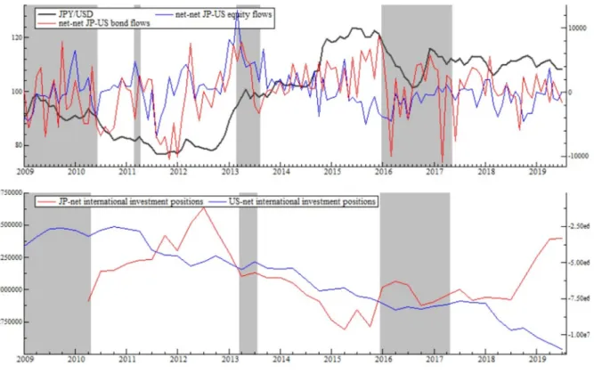
low-frequency requires averaging the high-frequency data, leading to the disappearance of some of the rapid market reactions to the differential variables. Against this limitation, we try to have a close look at the events causing high volatility over the sample and noting the direction of capital flows inducing changes in the JPY/USD exchange rate. To do so, we rely on monthly bilateral data on the Japanese-US capital flows provided by the Treasury International Capital (TIC) system disaggregated based on the type of the capital flows (such as stocks, bonds) and also quarterly international portfolio investment flows data provided by the IMF (See Figure 4).
One of the periods of excessive foreign exchange market volatility prevails from the beginning of the sample in 2009 until mid-2010, during which financial markets were still turbulent after the global financial crisis (see Figure 4 and the regime classifications in Table A 5). The upper panel of Figure 4 shows that during this period, an increasing (decreasing) net-net equity flows (defined as the net equity inflows into Japan minus the net equity inflows into the US) are associated with an appreciation (depreciation) of the JPY against the USD.
The short period of high volatility from March to May 2011 was caused by the earthquake and the heightened worries of the nuclear crisis in Japan. Instability in the Japanese stock market soared, and the JPY depreciated vis-à-vis major currencies. The disorderly foreign exchange market was very soon stabilized thanks to the concerted foreign exchange market intervention by G7 countries. The same negative relationship exists between the net-net equity flows and the exchange rate returns (Figure 4).
The next period of excess foreign exchange market volatility, which started in March 2013 and continued for around five months, was provoked by the implementation of a very intense monetary stimulus in Japan. The purpose of the stimulus was to defeat Japan’s continued deflation and to achieve a targeted inflation rate of two percent in the next two years. Subsequently, the BoJ’s balance sheet experienced a rapid expansion, the Japanese stock market rallied, and the yen depreciated. This monetary policy change was followed by a massive quantitative easing program in April 2013, in response to which financial market uncertainty increased, the JPY experienced further depreciation, and the stock market surged. However, skepticism about Abe’s expansionary policies coupled with some international news on the US tapering in May and June 2013 and China’s slowing growth caused an escalation of uncertainty in stock markets. Stock markets were hit both in Japan and the US, with a more striking effect in the former. The sudden drop of the net-net equity flows into Japan during this period (the third shaded area in Figure 4) is associated with higher uncertainty in the Japanese market and depreciation of this country’s currency, consistent with our hypothesis.
21 There are at least two sources of high-frequency data on capital flows, none of which is accessible freely. EPFR
dataset contains weekly portfolio investment flows at mutual funds level. IIF also provides net private capital inflows at a daily frequency.
20
The next series of events giving rise to heightened volatility in the JPY/USD exchange rate and uncertainty in different countries started in late 2015. On the one hand, in December 2015, US interest rates began to increase, accompanied by signals of further gradual increases during the following years. One the other hand, the BoJ adopted a negative interest rate policy in late January 2016 to stimulate investment and borrowing as well as boosting inflation and weakening the currency. In both cases, uncertainty around the consequences of the moves caused plunges in major, and sometimes in emerging markets. As a result, flight to safety by international investors and repatriation of Japanese overseas investments caused reinforcement of the safe-haven status of the JPY, and the Japanese yen appreciated accordingly. Similarly, later events such as the news on China’s slowdown signals in February, and the Brexit referendum in June both contributed to a strong JPY vis-à-vis the USD. The presidential election in the US in November and an increase in the US target rate in December both led to surges in the value of the USD after long periods of high financial market instability and the JPY depreciation.
In this period of high volatility, in contrast to the previous three periods, a positive relationship
Figure 4 Capital flows and exchange rate
Notes: upper panel shows the JPY/USD exchange rate in black on the left axis, and monthly net-net Japan-US bilateral equity flows in blue, net-net Japan-US bilateral bond flows in red, on the right axis. Lower panel shows quarterly net international investment inflows to Japan in red and net international investment inflows to the US in blue. Shaded areas are classified in the second regime by our selected model (the shaded area in March 2011 disappears in the lower panel due to its short duration and a lower frequency of the data).
21
exists between the net-net equity flows and the exchange rate returns. Therefore, at the first look, it might seem that relatively higher volatility in Japan does not lead to the depreciation of the JPY. But, given the specific status of the Japanese yen and the US dollar as safe-haven currencies, it may not be enough to only take into account the Japanese-US bilateral equity flows. As shown in the lower panel of Figure 4, during this period, gross inflows to Japan increased until mid-2016 and decreased afterward, while the opposite happens to the gross inflows to the US. Therefore, the JPY appreciates until midway in the period and then depreciates against the USD.
4
Conclusion
In this study, we explored for the first time the relationship between relative uncertainties in two countries’ stock markets and their corresponding exchange rate returns. We also examined the explanatory power of some of the previously-proposed determinants of the exchange rate dynamics, namely the stock returns differential and the differential of the growth of unconventional monetary policy measures.
Using a Markov-switching model and focusing on the JPY/USD exchange rate from 2009 to 2019, we show that our proposed determinant, the IV differential has a significant relationship with the exchange rate dynamics in our sample. Moreover, we document that the stock returns differential is an essential non-switching determinant of the JPY/USD exchange rate returns as consistent with UEP (Cappiello and De Santis, 2005; Hau and Rey, 2006). The differential of the relative increase in UMP of the two corresponding countries also plays a crucial nonlinear role in explaining the JPY/USD dynamics with one and two weeks of lag. Our unique findings emphasize the importance of the choice of sample based on corresponding countries' monetary stances.
A serious examination of the role of capital flows, as the transmission mechanism of the effects of the IV differential, stock returns differential, and reserves growth differential on exchange rate remains as a future extension of this study. Also, a comparison of findings using alternative uncertainty measures such as the EPU index can be very informative.
REFERENCES
Adler, M., Dumas, B., 1983. International portfolio choice and corporation finance: A synthesis. J. Finance 38, 925–984. https://doi.org/10.1111/j.1540-6261.1983.tb02511.x
Aloosh, A., 2014. Global variance risk premium and forex return predictability (No. 59931), Munich Personal RePEc Archive. University Library of Munich, Germany.
Andrews, D.W.K., Ploberger, W., 1994. Optimal tests when a nuisance parameter is present only under the alternative. Econometrica 62, 1383. https://doi.org/10.2307/2951753
Arbatli, E., Davis, S., Ito, A., Miake, N., Saito, I., 2017. Policy uncertainty in Japan. IMF Work. Pap. 17, 1. https://doi.org/10.5089/9781484300671.001
22
Bachmann, R., Elstner, S., Sims, E.R., 2013. Uncertainty and economic activity: Evidence from business survey data. Am. Econ. J. Macroecon. 5, 217–249. https://doi.org/10.1257/mac.5.2.217 Badshah, I.U., Frijns, B., Tourani-Rad, A., 2013. Contemporaneous spill-over among equity, gold, and exchange rate implied volatility indices. J. Futur. Mark. 33, 555–572. https://doi.org/10.1002/fut.21600
Baele, L., Bekaert, G., Inghelbrecht, K., Wei, M., 2018. Flights to safety. SSRN Electron. J. https://doi.org/10.2139/ssrn.3204192
Bai, J., Perron, P., 2003. Computation and analysis of multiple structural change models. J. Appl. Econom. 18, 1–22. https://doi.org/10.1002/jae.659
Baker, S.R., Bloom, N., Davis, S.J., 2016. Measuring economic policy uncertainty. Q. J. Econ. 131, 0–52. https://doi.org/10.1093/qje/qjw024.Advance
Balakrishnan, R., Goncalves, F.M., 2008. Financial flows from the United States to latin Amercia: Basic patterns, causes, and implications, in: Mühleisen, M., Roache, S.K., Zettelmeyer, J. (Eds.), Who’s Driving Whom? Analyzing External and Intra-Regional Linkages in the Americas. International Monetary Fund, Washington, DC. https://doi.org/10.5089/9781589067882.087 Balakrishnan, R., Laseen, S., Pescatori, A., 2016. U.S. dollar dynamics: How important are policy divergence and FX risk premiums? IMF Work. Pap. 16, 1. https://doi.org/10.5089/9781498348416.001
Bank for International Settlements, 2019. Triennial Central Bank Survey of Foreign Exchange Turnover in April 2019.
Bauer, M.D., Rudebusch, G.D., 2014. The signaling channel for Federal Reserve bond purchases. Int. J. Cent. Bank. 10, 233–289. https://doi.org/10.24148/wp2011-21
Bekaert, G., Hoerova, M., Lo Duca, M., Adrian, T., Amisano, G., DeJong, D., Mackowiak, B., Smets, F., Valentim, J., 2013. Risk, uncertainty and monetary policy. J. Monet. Econ. 60, 771– 788. https://doi.org/10.1016/j.jmoneco.2013.06.003
Bloom, N., 2014. Fluctuations in Uncertainty. J. Econ. Perspect. 28, 153–176. https://doi.org/10.1257/jep.28.2.153
Bollerslev, T., Tauchen, G., Zhou, H., 2009. Expected stock returns and variance risk premia. Rev. Financ. Stud. 22, 4463–4492. https://doi.org/10.1093/rfs/hhp008
Boscaljon, B., Clark, J., 2013. Do large shocks in VIX signal a flight-to-safety in the gold market? J. Appl. Financ. 23, 120–131.
Brunnermeier, M.K., Pedersen, L.H., 2009. Market liquidity and funding liquidity. Rev. Financ. Stud. 22, 2201–2238. https://doi.org/10.1093/rfs/hhn098
23
Caballero, R.J., Krishnamurthy, A., 2008. Collective risk management in a flight to quality episode. J. Finance 63, 2195–2230. https://doi.org/10.1111/j.1540-6261.2008.01394.x
Caporale, G.M., Karanasos, M., Yfanti, S., 2019. Macro-financial linkages in the high-frequency domain: The effects of uncertainty on realized volatility (No. 8000), Social Science Research Network, CESifo Working Paper. Munich Society for the Promotion of Economic Research- CESifo.
Cappiello, L., De Santis, R.A., 2007. The uncovered return condition (No. 812), Working Paper Series. European Central Bank, Frankfurt.
Cappiello, L., De Santis, R.A., 2005. Explaining exchange rate dynamics: The uncovered equity return parity condition (No. 529), Working Paper Series. European Central Bank.
Carrasco, M., Hu, L., Ploberger, W., 2014. Optimal test for Markov switching parameters. Econometrica 82, 765–784. https://doi.org/10.3982/ECTA8609
Carriero, A., Clark, T.E., Marcellino, M., 2018. Measuring uncertainty and its impact on the economy. Rev. Econ. Stat. 100, 799–815. https://doi.org/10.1162/rest_a_00693
Cenedese, G., Payne, R., Sarno, L., Valente, G., 2016. What do stock markets tell us about exchange rates? Rev. Financ., DP 20, 1045–1080. https://doi.org/10.1093/rof/rfv032
Chauvet, M., Senyuz, Z., Yoldas, E., 2015. What does financial volatility tell us about macroeconomic fluctuations? J. Econ. Dyn. Control 52, 340–360. https://doi.org/10.1016/j.jedc.2015.01.002
Cho, J.W., Choi, J.H., Kim, T., Kim, W., 2016. Flight-to-quality and correlation between currency and stock returns. J. Bank. Financ. 62, 191–212. https://doi.org/10.1016/j.jbankfin.2014.09.003 Chow, G.C., Lin, A., 1971. Best linear unbiased interpolation, distribution, and extrapolation of time series by related series. Rev. Econ. Stat. 53, 372. https://doi.org/10.2307/1928739
Curcuru, S.E., Thomas, C.P., Warnock, F.E., Wongswan, J., 2014. Uncovered equity parity and rebalancing in international portfolios. J. Int. Money Financ. 47, 86–99. https://doi.org/10.1016/j.jimonfin.2014.04.009
Davies, R.B., 1987. Hypothesis testing when a nuisance parameter is present only under the alternative. Biometrika 74, 33–43. https://doi.org/10.1093/biomet/74.1.33
Della Corte, P., Ramadorai, T., Sarno, L., 2016. Volatility risk premia and exchange rate predictability. J. financ. econ. 120, 21–40. https://doi.org/10.1016/j.jfineco.2016.02.015
Dempster, A.A.P., Laird, N.M., Rubin, D.B., 1977. Maximum likelihood from incomplete data via the EM algorithm. J. R. Stat. Soc. Ser. B 39, 1–38.
24
Dickey, D.A., Fuller, W.A., 1979. Distribution of the estimators for autoregressive time series with a unit root. J. Am. Stat. Assoc. 74, 427–431. https://doi.org/10.1080/01621459.1979.10482531 Ferrara, L., Lhuissier, S., Tripier, F., 2017. Uncertainty fluctuations: Measures, effects and macroeconomic policy challenges (No. 20), Policy Brief. CEPII. https://doi.org/10.1007/978-3-319-79075-6_9
Ferrara, L., Marsilli, C., Ortega, J.P., 2014. Forecasting growth during the Great Recession: Is financial volatility the missing ingredient? Econ. Model. 36, 44–50. https://doi.org/10.1016/j.econmod.2013.08.042
Fratzscher, M., 2012. Capital flows, push versus pull factors and the global financial crisis. J. Int. Econ. 88, 341–356. https://doi.org/10.1016/j.jinteco.2012.05.003
Fratzscher, M., Lo Duca, M., Straub, R., 2018. On the international spillovers of US quantitative easing. Econ. J. 128, 330–377. https://doi.org/10.1111/ecoj.12435
Fuertes, A.-M., Phylaktis, K., Yan, C., 2019. Uncovered equity “disparity” in emerging markets. J. Int. Money Financ. 98, 102066. https://doi.org/10.1016/j.jimonfin.2019.102066
Gagnon, J., Raskin, M., Remache, J., Sack, B., 2011. The financial market effects of the federal reserve’s large-scale asset purchases. Int. J. Cent. Bank. 7, 3–43.
Gilchrist, S., Sim, J., Zakrajšek, E., 2014. Uncertainty, financial frictions, and investment dynamics, Antimicrobial Agents and Chemotherapy. Cambridge, MA. https://doi.org/10.3386/w20038
Glick, R., Leduc, S., 2012. Central bank announcements of asset purchases and the impact on global financial and commodity markets. J. Int. Money Financ. 31, 2078–2101. https://doi.org/10.1016/j.jimonfin.2012.05.009
Hamilton, J.D., 1989. A new approach to the economic analysis of nonstationary time series and the business cycle. Econometrica 57, 357. https://doi.org/10.2307/1912559
Harada, K., Okimoto, T., 2019. The BOJ’s ETF purchases and its effects on Nikkei 225 stocks (No. 19- E- 014), Discussion Paper Series. RIETI.
Hau, H., Rey, H., 2008. Global portfolio rebalancing under the microscope (No. 14165), NBER Working Paper Series. National Bureau of Economic Research, Cambridge, MA. https://doi.org/10.3386/w14165
Hau, H., Rey, H., 2006. Exchange rates, equity prices, and capital flows. Rev. Financ. Stud. 19, 273–317. https://doi.org/10.1093/rfs/hhj008
Jo, S., Sekkel, R., 2019. Macroeconomic uncertainty through the lens of professional forecasters. J. Bus. Econ. Stat. 37, 436–446. https://doi.org/10.1080/07350015.2017.1356729
25
Joëts, M., Mignon, V., Razafindrabe, T., 2017. Does the volatility of commodity prices reflect macroeconomic uncertainty? Energy Econ. 68, 313–326. https://doi.org/10.1016/j.eneco.2017.09.017
Jubinski, D., Lipton, A., 2013. VIX, gold, silver, and oil: How do commodities react to financial market volatility? J. Account. Financ. 13, 70–88.
Jurado, K., Ludvigson, S.C., Ng, S., 2015. Measuring uncertainty. Am. Econ. Rev. 105, 1177– 1216. https://doi.org/10.1257/aer.20131193
Kenourgios, D., Papadamou, S., Dimitriou, D., 2015. On quantitative easing and high frequency exchange rate dynamics. Res. Int. Bus. Financ. 34, 110–125. https://doi.org/10.1016/j.ribaf.2015.01.003
Kim, H., 2011. The risk adjusted uncovered equity parity. J. Int. Money Financ. 30, 1491–1505. https://doi.org/10.1016/j.jimonfin.2011.06.020
Knight, F.H., 1921. Risk, uncertainty and profit, Houghton Mifflin Company. Houghton Mifflin Company, Boston and New York. https://doi.org/10.1017/CBO9781107415324.004
Krolzig, H.-M., 2003. General-to-specific model selection procedures for structural vector autoregressions. Oxf. Bull. Econ. Stat. 65, 769–801. https://doi.org/10.1046/j.0305-9049.2003.00088.x
Kwiatkowski, D., Phillips, P.C.B., Schmidt, P., Shin, Y., 1992. Testing the null hypothesis of stationarity against the alternative of a unit root. J. Econom. 54, 159–178. https://doi.org/10.1016/0304-4076(92)90104-Y
Le Moign, C., Raillon, F., 2018. Heightened volatility in early February 2018: The impact of VIX products. Autorité des Marchés Financiers.
Litterman, R.B., 1983. A random walk, Markov model for the distribution of time series. J. Bus. Econ. Stat. 1, 169. https://doi.org/10.2307/1391858
Londono, J.M., Zhou, H., 2017. Variance risk premiums and the forward premium puzzle. J. financ. econ. 124, 415–440. https://doi.org/10.1016/j.jfineco.2017.02.002
Markowitz, H., 1952. Portfolio selection. J. Finance 7, 77–91. https://doi.org/10.1111/j.1540-6261.1952.tb01525.x
Neely, C.J., 2015. Unconventional monetary policy had large international effects. J. Bank. Financ. 52, 101–111. https://doi.org/10.1016/j.jbankfin.2014.11.019
Nier, E., Saadi Sedik, T., Mondino, T., 2014. Gross private capital flows to emerging markets: Can the global financial cycle be tamed? IMF Work. Pap. 14, 1. https://doi.org/10.5089/9781498351867.001
26
Psaradakis, Z., Spagnolo, N., 2003. On the determination of the number of regimes in Markov-switching autoregressive models. J. Time Ser. Anal. 24, 237–252. https://doi.org/10.1111/1467-9892.00305
Rosa, C., 2012. How “unconventional” are large-scale asset purchases?
Sari, R., Soytas, U., Hacihasanoglu, E., 2011. Do global risk perceptions influence world oil prices? Energy Econ. 33, 515–524. https://doi.org/10.1016/j.eneco.2010.12.006
Sarwar, G., Khan, W., 2019. Interrelations of U.S. market fears and emerging markets returns: Global evidence. Int. J. Financ. Econ. 24, 527–539. https://doi.org/10.1002/ijfe.1677
Sarwar, G., Khan, W., 2017. The effect of US stock market uncertainty on emerging market returns. Emerg. Mark. Financ. Trade 53, 1796–1811. https://doi.org/10.1080/1540496X.2016.1180592
Smith, A., Naik, P.A., Tsai, C.L., 2006. Markov-switching model selection using Kullback-Leibler divergence. J. Econom. 134, 553–577. https://doi.org/10.1016/j.jeconom.2005.07.005
Stulz, R.M., 1995. Chapter 6 International Portfolio Choice and Asset Pricing: An Integrative Survey. Handbooks Oper. Res. Manag. Sci. 9, 201–223. https://doi.org/10.1016/S0927-0507(05)80050-7
Ueda, K., 2012. The effectiveness of non-traditional monetary policy measures: The case of the bank of Japan. Japanese Econ. Rev. 63, 1–22. https://doi.org/10.1111/j.1468-5876.2011.00547.x Vayanos, D., 2004. Flight to quality, flight to liquidity, and the pricing of risk (No. 10327), NBER Working Paper Series. Cambridge, MA. https://doi.org/10.3386/w10327