Direct sizing and characterization of Energy Storage Systems in the Energy-Power plane

HAL Id: hal-02330732

https://hal.archives-ouvertes.fr/hal-02330732

Submitted on 24 Oct 2019

HAL is a multi-disciplinary open access

archive for the deposit and dissemination of

sci-entific research documents, whether they are

pub-lished or not. The documents may come from

teaching and research institutions in France or

abroad, or from public or private research centers.

L’archive ouverte pluridisciplinaire HAL, est

destinée au dépôt et à la diffusion de documents

scientifiques de niveau recherche, publiés ou non,

émanant des établissements d’enseignement et de

recherche français ou étrangers, des laboratoires

publics ou privés.

Direct sizing and characterization of Energy Storage

Systems in the Energy-Power plane

Javier M. Cabello, Xavier Roboam, Sergio Junco, Christophe Turpin

To cite this version:

Javier M. Cabello, Xavier Roboam, Sergio Junco, Christophe Turpin. Direct sizing and

charac-terization of Energy Storage Systems in the Energy-Power plane. Mathematics and Computers in

Simulation, Elsevier, 2018, 158, pp.2-17. �10.1016/j.matcom.2018.04.002�. �hal-02330732�

OATAO is an open access repository that collects the work of Toulouse

researchers and makes it freely available over the web where possible

Any correspondence concerning this service should be sent

to the repository administrator:

tech-oatao@listes-diff.inp-toulouse.fr

This is an author’s version published in:

http://oatao.univ-toulouse.fr/24153

To cite this version:

Cabello, Javier M. and Roboam, Xavier and Junco, Sergio

and Turpin, Christophe Direct sizing and characterization of

Energy Storage Systems in the Energy-Power plane. (2018)

Mathematics and Computers in Simulation, 158. 2-17. ISSN

0378-4754

Official URL:

Direct

sizing and characterization of Energy Storage Systems in the

Energy-Power

plane

Javier

M. Cabello

,

Xavier Roboam

_,

Sergio Junco

_,

Christophe Turpin

a_{Laboratorio de Automatización y Control (LAC), Universidad Nacional de Rosario, Ríobamba 245 Bis, Rosario, Argentina} b_{Laboratoire Plasma et Conversion d’Energie (LAPLACE), UMR5213-CNRS-INPT-UPS, Toulouse, France}

Abstract

This paper presents an original sizing method for Energy Storage Systems (ESS) based on directly matching their capabilities – as specified by their energy-power Safe Operation Area (SOA) in the Energy-Power (EP) plane – with the energy and power demand required to accomplish their missions. Starting from the system requirements and from an energy management strategy, the power demanded by a set of representative operating scenarios and its associated energy are calculated and represented as trajectories in the EP plane. The objective is to size the ESS such as its SOA contains these trajectories. Comparison between different technologies of Energy Storage Devices (ESDs) is possible using this SOA characterization. Special attention should be paid to compare specific SOAs across devices. Diverse energy management strategies can be synthesized in the EP plane where they can be compared and analyzed. The sizing method converges extremely fast and is suitable for its integration in an optimization loop. The method allows to determine directly and efficiently the technology and the size most appropriate (in terms of indicators such as mass or cost) to a given EP demand. In the paper, three different technologies (SuperCapacitor, Li-Ion and H2/O2batteries) are characterized and compared in terms of sizing synthesis.

Keywords: Energy storage systems; Sizing method; Energy vs power characterization

1. Introduction

Energy Storage Systems (ESSs) are key elements in electrical systems especially in hybrid systems or smart grids. They allow for increased integration of renewable energy sources connected to the grid [18,24] as well as to increase reliability, stability and resilience of various systems [3,10,15,17,19]. There are several kinds of ESSs technologies such as: Pumped Hydro Storage, Compressed-Air Energy Storage, Battery Energy Storage (BES), Capacitor Storage, Super-Capacitor Energy Storage (SCES), Super-Conducting Magnetic Energy Storage, Thermal

∗

Corresponding author.

E-mail addresses: jcabello@fceia.unr.edu.ar (J.M. Cabello), xavier.roboam@laplace.univ-tlse.fr (X. Roboam), sjunco@fceia.unr.edu.ar (S. Junco), turpin@laplace.univ-tlse.fr (C. Turpin).

Energy Storage, Hydrogen Energy Storage (HES), and Flywheel Energy Storage. Each technology has its benefits and its drawbacks [9,11,19]

The ESS technology selection is a critical stage in a system development. In this aspect the Ragone plot [8,21] is a well-known graphical characterization tool that exhibits the storage types differences in terms of their specific-power and specific-energy. Many other aspects are characterizing such as efficiency, durability, reliability, response time or power vs energy capability [11,19]. According to the application these aspects can be decisive in the early stages of technology selection.

An ESS can be constituted by just one or many Energy Storage Devices (ESDs), in the latter case, of a unique or of diverse technologies. These two situations are defined here as single and hybrid-technology ESS. In this paper only single-technology ESS is considered. Normally, an ESS is composed of a certain number of ESDs. The ESS sizing consists mainly in finding this number of ESDs in order to fulfill the system requirements. There are several sizing methods of high computational-cost requiring multiple simulations, such as Brute Force, Genetic Algorithm [2,22], and Efficient Global Optimization [22].

One method commonly used to size ESS is the maximum power and energy demand method. This simple method consists in taking into account the power span and energy span separately and size the ESS to supply these energy and power [4,13]. But this may result in an over-sizing of the ESS as the method treats the power and energy demand in an uncorrelated way.

In [20] a SCES system is sized based on the constant power discharge over a maximum time interval. In [23] the EP capabilities are taken into account to validate the sizing of a SCES by comparing it with the energy and power demand in the EP plane.

The present work combines the ESD characterization and the complete demand profile in the EP plane in order to match them and directly obtain the ESS size able to satisfy this demand [6].

The first stage of this sizing method is to characterize each ESD according to its EP capabilities. These capabilities are calculated from the limits of the ESD-variables (such as voltage limits, current limits, and state of charge limits) within which the device is expected to operate safely and is represented in an Energy vs Power plane: a SOA (Safe Operating Area) is consequently defined for each ESD. The second stage is the synthesis of a demand profile. Starting from the system requirements and from an energy management strategy, the power demanded by a set of representative operating scenarios and the associated energy are calculated and represented as trajectories in the EP plane, constituting the Demanded Energy-Power Trajectory (DEPT). The third and last stage is to size the ESS such that its SOA contains the DEPT assuring that the EP capabilities of the ESS are not exceeded.

It is worth mentioning that stages 1 and 2 are independent, a change in one does not affect the other. E.g. if a new ESD is to be tested the DEPT does not need to be recalculated; even more if the SOA of this new ESD was already obtained from a previous analysis, only the last stage should be performed reducing the total calculation cost.

The SOA may also be defined in specific EP plane by considering mass specific plane (in Wh/kg vs W/kg), which is of interest for embedded systems, or cost specific plane (in Wh/$ vs W/$), especially for stationary applications. This allows a rapid comparison between ESD (either of the same or different technologies) and realizing which one is more effective in terms of power/energy per specifying parameter (mass, cost, etc.).

The remainder of this work is organized as follows: Section 2 shows the Energy vs Power characterization particularized for the 3 energy storage technologies considered (SCES, BES and HES). In Section3the demanded profile synthesis is analyzed. Section 4 deals with the sizing procedure. In Section 5 the results of applying this method in 2 case studies with numerical validation (and experimental for case study 2) are shown. Finally the main conclusions are summarized in Section6.

2. Energy vs Power characterization of energy storage devices

ESDs can be characterized by their power capability which strongly depends on the State of Charge (SoC) and the safe operating limits of their variables, imposed by the manufacturer or also by the system designer.

Analogously to the commonly known voltage vs current Safe Operating Area,1_{the EP SOA (here after only SOA)} of an ESD can be defined as the EP conditions over which the device can be expected to operate without self-damage.

1_{The power semiconductor devices Safe Operating Area is defined by the voltage and the current conditions over which the device can be}

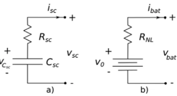
Fig. 1. (a) SuperCapacitor simplest model (capacity in series with a resistance) (b) Electrochemical battery simplified model.

Table 1

Parameters table of 3 Maxwell SC.

Module BMOD00 Csc(F) Rsc(m) Vmax(V) Imax(A)

58 E016 58 22 16 170

06 E160 5.8 220 160 170

83 P048 83 10 48 1150

This SOA can be calculated via physical experiments of the ESD or can be calculated using the ESD model with the corresponding parameterization. In the following subsections the model of 3 energy storage technologies are presented (SCES, BES and HES) and their SOAs calculated but, being generic, this concept can be extended to any ESS technology (flywheel, thermal or hydraulic storage, etc.).

2.1. SuperCapacitor 2.1.1. Model

The simplest SuperCapacitor (SC) model is a capacitance, Csc, in series with a resistance, Rsc, [20] seeFig. 1a.

For a given SC the variables limits are a minimum voltage, Vmi n, a maximum voltage, Vmax, and a maximum current

(for both, charge and discharge), Imax. Normally, Vmaxand Imaxare defined as the maximum nominal values rated by

the manufacturer but Vmi nis a system designer choice as it depends on the power electronic associated. The energy

stored in the SC can be calculated as Esc= 1₂CscVC sc2 . Using this equation the SoC is calculated as

SoCsc = Esc Esc−max = V 2 C sc V2 max (1)

2.1.2. SCES Energy vs Power SOA

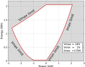
During a charging process at low SoC, the current limits the power input and, at high SoC, the maximum voltage does it. Inversely, at high SoC, the current limits the power output while the minimum voltage limit does it at low SoC. This can be summarized by the following equations. (SeeFig. 2.)

Psc−li m(Esc) =

VC sc(Esc) − Vsc−li m

Rsc

Vsc−li m (2)

Vsc−li m=

{min(Vmax, VCsc+RscImax) isc < 0

max(Vmi n, VCsc−RscImax, VCsc/2) otherwise

2.1.3. Different SOAs for different SCs

The first benefit of this Energy Power oriented storage characterization is the comparison between ESD of the same family but with very different voltage and current limits. Let us take for example 3 SC of Maxwell Technologies (see

Table 1).

Fig. 2. SOA for supercapacitor Maxwell 58F 16V.

Fig. 3. SOA for 3 supercapacitor.

2.2. Electrochemical battery 2.2.1. Model

There are several battery models of diverse complexity and accuracy. Here, the model extension of the commonly used analytic semi-empiric Tremblay–Dessaint battery model presented in [5] is used, which allows for an accurate reproduction of the battery output voltage without increasing the model complexity. It can be summarized as follows:

d dtSoC = − 1 Qi d dti ∗_{= −} 1 Tf i∗+ 1 Tf i vbat =E0+Ae−B Q(1−SoC)−K1Q ( ₁ SoC −1 ) −Ri − K2i∗ ( i sdch SoC + i sch 1.1 − SoC ) (3)

Table 2

Parameters table of Mottcell and SAFT batteries.

Parameter Saft-VL41M Mottcell Battery constant voltage E0(V) 3.24 3.26

Exponential zone amplitude A (mV) 750 74.5 Exponential zone inverse capacity Q (Ah) 0.03 0.033 Battery capacity Q (Ah) 41 36.8 Polarization constant K1(mV/Ah) 0.104 0.24

Polarization resistance K2(m) 0.104 0.747

Internal resistance R (m) 1.97 6.36 Current-filter time constant Tf (s) 30 88

where the variables are the battery discharge current i (A), the State of Charge SoC, the filtered discharge current i∗

(A) and the battery voltagevbat(V). The parameters are the battery capacity Q (Ah), the current-filter time constant Tf

(s), the battery constant voltage E0(V), the exponential-zone amplitude A (V) and exponential-zone inverse capacity

B(1/Ah), the polarization constant K1(V/Ah), the internal resistance R () and the polarization resistance K2().

The logic variables i sdch, being 1 when the battery is discharging and 0 otherwise, and i sch, being 1 when the battery

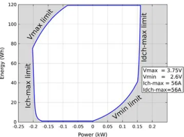
is charging and 0 otherwise, have been introduced to condense notation. 2.2.2. BES Energy vs Power SOA

Similarly to the SC, maximum and minimum voltages are Vmax and Vmi n respectively. For this particular

technology, distinction of the maximum current is normally done for charge and discharge processes (Ich−max and

Idch−max). In order to avoid premature aging SoC limitations (SoCmax and SoCmin) are also included. To calculate the

maximum charge and discharge powers the current dynamics are ignored and the voltage equation in(3)is simplified as in(4), assuming a source in series with a non-linear resistance, seeFig. 1b

vbat =v0−RN Libat v0(SoC) = E0+Ae−B Q(1−SoC)−K1Q ( ₁ SoC −1 ) (4) RN L(SoC) = R + K2 ( i sdch SoC + i sch 1.1 − SoC )

One particularity of this model (and in almost every battery model) is that the SoC represents the remaining charge in battery and not the energy stored. But there is a relation between them. Considering the non dissipative voltage, v0, the energy stored can be calculated as

Ebat(SoC) = Ei ni − ∫ t t0 v0(SoC)ibat(τ)dτ = Ei ni− ∫ SoC SoC0 v0(SoC)Qd SoC (5)

Similarly to Eq.(2), the power limits, as shown inFig. 4, can be calculated as Pbat −li m(Ebat) =

V0bat(Ebat) − Vbat −li m

RN L

Vbat −li m (6)

Vbat −li m =

{min(Vmax, v0+RN LIch−max) ibat < 0

max(Vmi n, v0−RN LIdch−max) otherwise

2.2.3. SOAs comparison between 2 batteries

In order to compare 2 Li-Ion batteries, defined inTable 2, we can plot both SOAs as displayed inFig. 5. 2.3. Hydrogen energy storage

An HES system is normally composed by an electrolyzer (ELYZ), a fuel cell (FC) and two tanks (Hydrogen and Oxygen) [20]. The ELYZ separates the water molecule (H2O) in the corresponding hydrogen (H2) and oxygen (O2)

Fig. 4. SOA for Li Ion battery Mottcell 36 Ah 3.2 V.

Fig. 5. SOA for 2 Li-Ion batteries.

are stored in tanks. Later on, the FC is in charge of combining these 2 gases and producing, once again, electrical energy, with water as a sub-product. Even though the physics involved in the electrochemical process (ELYZ and FC) is complicated and several complex models have been developed [12,20] for this particular stage only steady-state models are used.

In both ELYZ and FC, the base component is a cell. These cells can be combined in series (building a stack) and in parallel in order to obtain higher voltage and current capabilities, respectively. In both cases the base unit is the cell.

It is worth mentioning that in the case of a HES system the sizing of 3 components can be done independently, which provides a freedom of design that is missing in others ESD. Moreover, the maximum power of charge and discharge are independent of the SoC given by the amount of moles of H2/O2in the tanks.

2.3.1. Electrolyzer model

The ELYZ cell steady state behavior, i.e. the V–I polarization curve [12], is approximated by a straight line. The cell uses a considerable amount of electrical power in the auxiliary system composed mainly of compressors and the cooling system. This auxiliary consumption is approximated as a constant power consumption plus a power

consumption proportional to the cell power. From a given ELYZ base system (auxiliary + 1 cell) the maximum input power can be calculated as

Pi n−cellE LY Z −M A X =[(1 + kauxE LY Z) pcellE LY Z −M A X +paux mi nE LY Z] ScellE LY Z (7)

where Pi n−cellE LY Z −M A X is the maximum ELYZ system input power per cell (W), pcell E LY Z −M A X is the maximum

ELYZ cell power density (W/cm2), paux mi nE LY Z is the constant ELYZ auxiliary power density (W/cm

2_{), k}

auxE LY Z is

the proportional ELYZ auxiliary coefficient and ScellE LY Z is the ELYZ cell surface (cm

2_).

2.3.2. Fuel cell model

Similarly, the FC uses a considerable amount of electrical power obtained from the conversion process in the auxiliary system composed also mainly by compressors and the cooling system. The rest of the power is effectively usable electrical power. The linear approximation of the FC’s V–I polarization curve presented in [12] is considered here.

The auxiliary power consumption is approximated as a constant consumption plus a consumption proportional to the cell power. From a given FC (auxiliary + 1 cell) the maximum output power per cell can be calculated as

Pout −cellF C −M A X =[(1 − kauxF C) pcellF C −M A X−paux mi nF C] ScellE LY Z (8)

where Pout −cellF C −M A X is the maximum FC output power per cell (W), pcellF C −M A X is the maximum FC cell power

density (W/cm2_{), p}

aux mi nF C is the constant FC auxiliary power density (W/cm

2_{), k}

auxF C is the proportional FC

auxiliary coefficient and Scell_{F C} is the FC cell surface (cm2).

2.3.3. Tank model

The Hydrogen tank has a defined volume (Vt ank). Considering the ideal gas model, the pressure in the tank ( pt ank)

can be calculated from the number of moles nH2as

pt ank=

nH2RT

Vt ank

(9) where R is the ideal gas constant (8.3144598 J mol−1_K−1_{) and T is the temperature (K).}

Both gases (H2and O2) produced in the electrolysis process are stored in tanks. As the number of Hydrogen moles

formed is the double of the Oxygen moles, the size of the Hydrogen tank is the double of the Oxygen one in order to obtain the same pressure evolution during the charge and discharge processes.

2.3.4. HES Energy vs Power SOA

As mentioned in Section 2.3 the charge and discharge power limits and the energy stored are completely independent and can be calculated as

Phess−li m =

{ Pout −cellF C −M A X if discharge

−Pi n−cellE LY Z −M A X if charge

(10) while the maximum usable energy stored (Ehess−max) can be calculated as

Ehess−max =nH₂EH₂MH₂ =

( pt ank−M A X−pt ank−M I N)Vt ankEH2MH2

RT (11)

where EH₂ is the specific energy of the Hydrogen (39.7 kWh/kg2) and MH₂ is the Hydrogen molar mass.

Fig. 6shows the SOA of the HES system composed by an ELYZ cell, a FC cell and an Hydrogen tank parameterized from the data in [12].

2.4. Absolute and specific SOA

Fig. 7compares the SOA of the 6 ESD analyzed so far with 3 different technologies. We can see the differences between them. The HES systems are clearly the most energetic technology. Lithium Ion Batteries are less energetic than HES but more powerful. While the SC are the most powerful technology even though they are not so energetic.

Fig. 6. SOA of an HES (Hydrogen Power [12]).

Fig. 7. Absolute SOA plots of the ESDs analyzed: 3 SC, 2 Li-Ion batteries and 1 HES.

But in order to truly compare ESD, it is not fair to compare different technologies, or even elements of the same technology but with different sizes, in absolute SOAs displaying absolute EP plane. For instance, which SC is better, the BMOD0058 E016 B02 or the BMOD0006 E160 B02? One solution to make this comparison is the specification of the SOA by choosing a parameter (e.g. mass) and dividing the absolute SOA by this parameter.

This concept is already used in the well-known Ragone plots [8,21]. In the Ragone plot, the ESD is characterized by the available mass-specific energy (in kWh/kg) for mass-specific constant active power request (in kW/kg). When overlapping several ESD plots, each storage technology defines a region in the mass-specific energy and mass-specific power plane. Such vision related to the device mass (or volume) is all the more relevant for embedded systems.

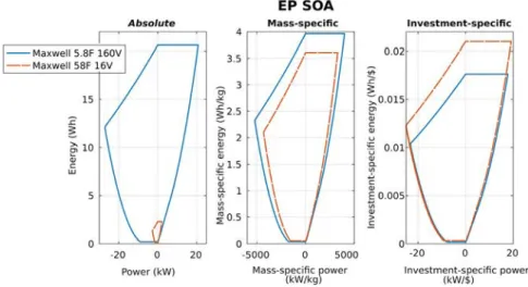
The specific SOAs allow us to compare the ESD by different parameters. Take for example 2 SC (SC160V =

BMOD0006 E160 B02 and SC16V = BMOD0058 E016 B02), both absolute SOAs are quite different, Fig. 8a.

Nevertheless it is not the case if we consider the energy and power per mass or per investment, Figs. 8b and8c.

Comparing the Mass-specific SOA of both SC it can be seen that SC160Vis better from the mass point of view (more

energy and power available per kg). On the contrary, from the economical point of view SC16V is more advantageous

(more energy and power per dollar invested). This vision related to the cost is often more relevant in stationary applications while the mass criteria are often the prime target for embedded systems.

Fig. 8. 2 SC devices (a) SOAs (b) Mass-specific SOAs and (c) Investment-specific SOAs.

Fig. 9. (a) Mass-specific SOAs and (b) Investment-specific SOAs.

Fig. 9summarizes the mass-specific and investment-specific SOAs for the 6 ESD analyzed. The technology regions shown in both specific EP planes reveal, for example, the predominant feature of SC as power storage systems instead of energy ones.

3. Demanded profile synthesis

Starting from the system requirements and from an energy management strategy (e.g. ESS associated to a renewable generator farm in order to reduce curtailment) a power profile along with the associated energy demanded to the ESS is obtained. This allows not only to analyze the demanded energy and power span, and their correlation, but also rapidly synthesize and compare different management strategies as shown in case study 2.

3.1. Demanded energy and power plots

Starting from a power demand, Pdem, the demanded energy, Edem, can be easily calculated as its integral. As the

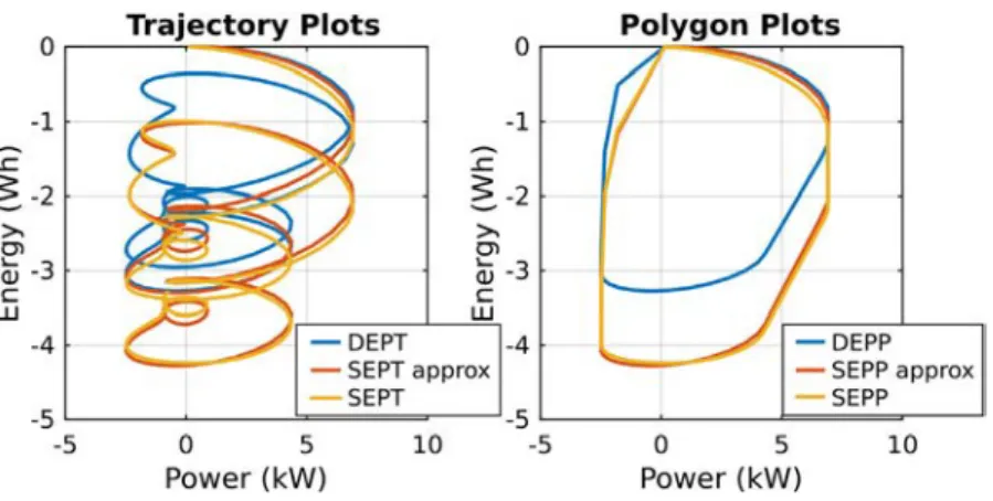
Fig. 10. Comparison in a SC between D E P, S E P and S E Pappr ox(a) Trajectories and (b) Polygons.

variation demanded to the ESS as, Edem(t ) = −

∫

Pdem(t )dt (12)

Plotting these two variables in the EP plane defines the Demanded Energy vs Power Trajectory (DEPT) that correlates both demands. The convex polygon circumscribing the DEPT is the Demanded Energy vs Power Polygon (DEPP) representing the demanded working area. In order to perform the calculation of the convex polygon (DEPP) of a given set of points (the DEPT in this case) the gift wrapping algorithm, a.k.a. Jarvis March algorithm, was implemented [16]. This synthesis reduced the amount of data to be used in the sizing stage (polygon fitting).

3.2. Approximated storage EP plots

The demanded energy of an ESS is not the same as its internal energy variation due to its losses. But the actual losses of the ESS can only be calculated once its size is defined. In order to break this implicit loop, constant efficiency (in charge,ηch, and discharge,ηdch) ESS models are considered. The internal storage energy variation, Est or age, is

calculated as: Est or age(t ) = − ∫ k Pdem(t )dt (13) k = { ηch Pdem ≤0 1/ηdch Pdem > 0

Following, the Storage Energy vs Power Trajectory Approximation (S E P Tappr ox) and the Storage Energy vs Power

Polygon Approximation (S E P Pappr ox) are defined using Est or ageinstead of Edem. The ESDs of the same family have

similar efficiencies (SCES around 98%, BES around 97% and HES around 50%–60% only without co-generation) even though they depend on the storage usage.

Both, the model complexity reduction (constant efficiency model) and the reuse of S E P Pappr ox(and S E P Tappr ox)

of same efficiency ESD, are the main sources of computational cost reduction. 3.3. Storage energy power plots

Once the ESD is selected and the ESS sized, the true internal energy variation given the demanded power can be calculated and both, S E P T and S E P P, obtained. When constant efficiency values (according to the ESD) are correctly chosen, both S E P Tappr oxand S E P T remain close asFig. 10shows for a SC.

4. Sizing procedure

The objective is to synthesize an ESS composed of multiple ESD units able to supply the demanded power profile without exceeding their safe operating capabilities: in other words, the S E P T should remain inside the

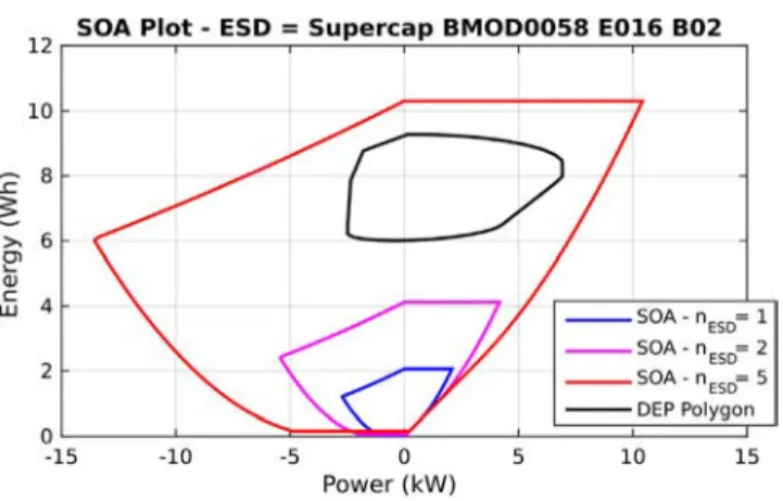
Fig. 11. Sizing procedure: ESS-SOA variation with the number of ESD and polygon fitting.

ESS-SOA. The sizing procedure then consists in increasing the number of ESD units until the S E P T fits inside the ESS-SOA.

4.1. ESS-SOA

It can be demonstrated that the SOA of an ESS composed by nE S Dunits is the same SOA of this ESD scaled by a

factor nE S D. From the EP point of view it does not matter the connection type (series or parallel) of the ESDs.

4.2. Polygon fitting

The size of the ESS will be the minimum value of ESD units (nE S D) such as the S E P P remains inside the

ESS-SOA. As mentioned in the previous section, this gives rise to a looped process, as in order to really know the S E P P the ESS size should be known. This looped process may lead to a great simulation cost depending on the model complexity. A solution to this problem is to use the approximated S E P P (S E P Pappr ox) instead of the exact S E P P,

avoiding the need of simulating each new size and allowing for a fast calculation. For each nE S D the ESS-SOA is

easily calculated and then tested if the S E P Pappr oxfits inside.Fig. 11exemplifies this sizing procedure.

5. Validation cases

The method is paradigmatically presented on two case studies. For the first one, a simple energy management is selected (E M1) and 3 ESD technologies are evaluated in order to make a technological comparison of sizes: Maxwell

SC BMOD0058 E016 B02, Mottcell 12 V 36 Ah LiIon and Hydrogen Power HES system from [12]. The second case takes into account 3 different energy management strategies (E M1, E M2 and E M3) and only one ESD technology

(Maxwell SC BMOD0058 E016 B02) in order to exhibit the influence of the energy management in the sizing process.

5.1. System requirements

The system consists of a reduced scale 450 W wind generation turbine connected to the grid with production commitment on the day ahead market [14]. Note that this strongly reduced case study has been defined aiming at a later validation of the synthesis process on a reduced scale test-bench. The microgrid is committed to delivering a power profile equal to the predicted wind power generation, Peng. Naturally, the real power production, Ppr od, is not

equal to the forecast. The ESS will be used to keep the grid transfer equal to Pengor within a certain tolerance band

Fig. 12. (Top plot) Wind turbine power prediction, Peng, and real generation, Ppr od. (Bottom plot) Power demanded to the ESS, Pdem, for the 3

EM strategies (E M1, E M2, E M3).

5.2. Energy management strategies

The simplest strategy, E M1, does not consider any tolerance band. Thus, the power demanded to the storage, Pdem,

is the difference between the committed power, Peng, and the actual one, Ppr od. Meaning that the ESS will be used

practically all the time. When a power tolerance, Pt ol, is allowed, several energy management strategies could be

defined. E M2consists in using the ESS only when the tolerance band is exceeded, i.e., as less as possible. For E M3,

the last energy management the ESS charging stage (when Pdem < 0) has been increased in order to reduce the energy

span of the Demanded Trajectory allowing a smaller ESS as can be seen in Case 2. Whenever Ppr od is greater than

Peng, Pdemwill be equal to Peng−Ppr od. The 3 strategies are summarized as follows:

E M1:Pdem =Peng−Ppr od (14) E M2:Pdem = ⎧ ⎨ ⎩ Peng−Pt ol−Ppr od i f Ppr od< Peng−Pt ol Peng+Pt ol−Ppr od i f Ppr od> Peng+Pt ol 0 ot herwise (15) E M3:Pdem = ⎧ ⎨ ⎩ Peng−Pt ol−Ppr od i f Ppr od< Peng−Pt ol Peng−Ppr od i f Ppr od> Peng 0 ot herwise (16) 5.3. Case study 1

5.3.1. Demanded profile synthesis

In this particular case the strategy E M1 is selected.Fig. 13depicts the S E P Tappr ox and S E P Pappr ox obtained

considering constant efficiency models for the 3 technologies (SCES with 98%, BES with 97% and HES with 50%). 5.3.2. Polygon fitting

Using the SOAs from the 3 ESD and the S E P Tappr oxcalculated in the previous stage, the sizing process indicates

that 11 SC BMOD0058 or 1 Mottcell are necessary to fulfill the power demand. In the case of HES system, 1 ELYZ cell and 1 FC cell are enough to achieve the power demand; and a tank of 0.72 dm3to achieve the energy demand. 5.3.3. Experimental validation

First, these sizes were validated by simulation verifying that the S E P T remains close to the S E P Pappr oxand none

of the ESS limits were exceeded.

Additionally the solution with SC and BES was also tested in real physical implementation. In order to test them, the power profile demanded to the ESS is emulated on a remote controllable bidirectional source of voltage/current

Fig. 13. S E P Tappr oxand S E P Pappr oxfor the wind turbine generation system for the 3 technologies analyzed: SCES, BES and HES.

Fig. 14. Overlapping of ESS-SOAs, S E P Pappr ox, simulated SEPT and physically tested SEPT.

(configured by a Power source PSI 9080-510 and a Controlled Load ELR 9080-510) using a dSPACE system. Over-and under-voltage protections, as well as thermal protection are implemented. To obtain more accurate Over-and faster sampling rate a SEFRAM Data acquisition System with 3 Clamps on probe HIOKI 3274 is used. This test bench, used already in [7], allows for voltage, current and power control of user defined profiles, and measurements of each ESD voltage, up to 3 currents and several temperatures (environment, ESD terminals, body, etc.).

Fig. 14compares the S E P Pappr ox, the S E P T obtained via simulation and the S E P T obtained via physical

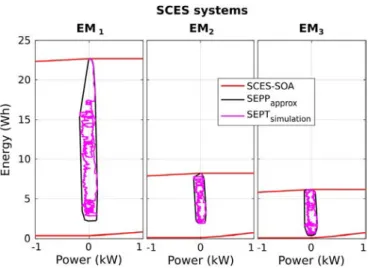
Fig. 15. S E P Tappr oxand S E P Pappr oxfor the wind turbine generation system for the 3 energy management strategies.

5.4. Case study 2

5.4.1. Demanded profile synthesis

The 3 energy management strategies presented with only one technology (SCES) were considered in this case study. The S E P Tappr ox and S E P Pappr ox were obtained considering, once more, equal charge and discharge efficiencies

(98% for SCES), as shown inFig. 15. A considerable reduction of energy demanded can be seen from E M1to E M2

(69% reduction) and a small reduction from E M2to E M3(9%).

5.4.2. Polygon fitting

Using the SOAs from the SCES and the results of the S E P Tappr oxof the previous stage, the sizing process indicates

that 11, 4 or 3 SC BMOD0058 Maxwell modules, using E M1, E M2and E M3respectively, are necessary to fulfill the

power profile demanded.

5.4.3. Simulation validation

These sizes were validated by simulation verifying that the S E P T remains close to the S E P Pappr oxand none of

the ESS limits were exceeded, as depicted inFig. 16.

6. Conclusion

A sizing method for ESS based on the EP plane has been proposed. This method separates the ESD characterization, the demanded profile synthesis and the strictly sizing stage. It is easy to add a new device to the analysis or to change the energy management strategy.

An important application of ESD characterization by the SOA is for comparing different types of storage devices in the early selection stages, considering different as well as a unique technology. In this paper, SC, Li-Ion batteries and Hydrogen–Oxygen storage have been considered for the technological analysis. Specific SOAs are very interesting in this comparison process as different criteria could be considered in terms of the specifying parameters (mass, price, volume, embodied energy, etc.).

In the Demanded Profile Synthesis several strategies can be compared and analyzed independently of the ESD selection as shown in the second case study. Critical areas or repeating patterns could be easily found in the Demanded Energy vs Power Trajectory plot. Furthermore, storage hybridization strategies can be analyzed by observing the obtained energy vs power plots for each storage element.

Fig. 16. Overlapping of the 3 of SCES-SOAs, S E P Pappr oxand simulated SEPT for the 3 EM.

Acknowledgments

This work was supported by the Argentine National Council for Scientific and Technological Research (CONICET) [Ph.D. Scholarship, 2013] and INP Toulouse France [Grant for International Mobility, 2016]. The authors would like to thank M.Sc.Eng. Eric Bru and Eng. Joaqu´ın Mauricio Pulido Aguilar for their support during the test-bench construction and testing.

References

[1] B. Adolph, Field-Effect and Bipolar Power Transistor Physics, Academic Press, 1981.

[2] C.R. Akli, B. Sareni, X. Roboam, A. Jeunesse, Integrated optimal design of a hybrid locomotive with multiobjective genetic algorithms, Int. J. Appl. Electromagn. Mech. 30 (2009) 151–162.

[3] C. Barreto, J. Giraldo, Á.A. Cárdenas, E. Mojica-Nava, N. Quijano, Control systems for the power grid and their resiliency to attacks, IEEE Secur. Priv. 12 (2014) 15–23.

[4] H. Bludszuweit, J.A. Domínguez-Navarro, A probabilistic method for energy storage sizing based on wind power forecast uncertainty, IEEE Trans. Power Syst. 26 (2011) 1651–1658.

[5] J.M. Cabello, E. Bru, X. Roboam, F. Lacressonniere, S. Junco, Battery dynamic model improvement with parameters estimation and experimental validation, in: Proceeding IMAACA 2015, the International Conference on Integrated Modeling and Analysis in Applied Control and Automation, Bergeggi, Italy, pp. 3–70.

[6] J.M. Cabello, X. Roboam, S. Junco, A direct sizing method and specific characterization of energy storage devices/systems in the energy vs power plane, in: Proceeding ELECTRIMACS 2017, Toulouse, France.

[7] J.M. Cabello, X. Roboam, S. Junco, E. Bru, F. Lacressonniere, Scaling electrochemical battery models for time-accelerated and size-scaled experiments on test-benches, IEEE Trans. Power Syst. 32 (2017) 4233–4240.

[8] T. Christen, M.W. Carlen, Theory of ragone plots, J. Power Sources 91 (2000) 210–216.

[9] A. Dekka, R. Ghaffari, B. Venkatesh, B. Wu, A survey on energy storage technologies in power systems, in: Electrical Power and Energy Conference, EPEC, IEEE, 2015, pp. 105–111.

[10] P. Du, N. Lu, Energy Storage for Smart Grids: Planning and Operation for Renewable and Variable Energy Resources (VERs), Academic Press, 2014.

[11] H.L. Ferreira, R. Garde, G. Fulli, W. Kling, J.P. Lopes, Characterisation of electrical energy storage technologies, Energy 53 (2013) 288–298. [12] F. Gailly, Alimentation électrique d’un site isolé à partir d’un générateur photovoltaïque associé à un tandem électrolyseur/pile à combustible

(Batterie H2/O2) (Ph.D. thesis), Institut National Polytechnique de Toulouse, 2011.

[13] D.W. Gao, H. Babazadeh, L. Lin, A practical sizing method of energy storage system considering the wind uncertainty for wind turbine generation systems, in: Green Technologies Conference, IEEE, IEEE, 2013, pp. 127–133.

[14] D. Hernandez-Torres, C. Turpin, X. Roboam, S.,B., Optimal techno-economical storage sizing for wind power producers in day-ahead markets for island networks, in: Proceeding ELECTRIMACS 2017, Toulouse, France.

[15] IEEE guide for the interoperability of energy storage systems integrated with the electric power infrastructure, IEEE Std 2030.2-2015, pp. 1–138.

[17] G.L. Kyriakopoulos, G. Arabatzis, Electrical energy storage systems in electricity generation: energy policies, innovative technologies, and regulatory regimes, Renew. Sustain. Energy Rev. 56 (2016) 1044–1067.

[18] F. Lamberti, V. Calderaro, V. Galdi, G. Graditi, Massive data analysis to assess PV/ESS integration in residential unbalanced LV networks to support voltage profiles, in: Electric Power Systems Research, Vol. 143, 2017, pp. 206–214.

[19] O. Palizban, K. Kauhaniemi, Energy storage systems in modern grids—matrix of technologies and applications, J. Energy Storage 6 (2016) 248–259.

[20] M.C. Pera, D. Hissel, H. Gualous, C. Turpin, Electrochemical Components, John Wiley & Sons, 2013.

[21] D.V. Ragone, Review of Battery Systems for Electrically Powered Vehicles, Technical Report, SAE Technical Paper, 1968.

[22] R. Rigo-Mariani, B. Sareni, X. Roboam, Integrated optimal design of a smart microgrid with storage, IEEE Trans. Smart Grid 8 (2017) 1762–1770.

[23] X. Roboam, O. Langlois, H. Piquet, B. Morin, C. Turpin, Hybrid power generation system for aircraft electrical emergency network, IET Electr. Syst. Transp. 1 (2011) 148–155.

[24] H. Zhao, Q. Wu, S. Hu, H. Xu, C.N. Rasmussen, Review of energy storage system for wind power integration support, Appl. Energy 137 (2015) 545–553.