6. Static and dynamic properties of topological defects in ultrathin films and dots

HAL Id: hal-01166224

https://hal.archives-ouvertes.fr/hal-01166224

Submitted on 22 Jun 2015

HAL is a multi-disciplinary open access

archive for the deposit and dissemination of sci-entific research documents, whether they are pub-lished or not. The documents may come from teaching and research institutions in France or abroad, or from public or private research centers.

L’archive ouverte pluridisciplinaire HAL, est destinée au dépôt et à la diffusion de documents scientifiques de niveau recherche, publiés ou non, émanant des établissements d’enseignement et de recherche français ou étrangers, des laboratoires publics ou privés.

in ultrathin films and dots

Jean-Claude Serge Levy

To cite this version:

Jean-Claude Serge Levy. 6. Static and dynamic properties of topological defects in ultrathin films and dots. Jean-Claude Serge Lévy. Nanostructures and their magnetic properties, S.G. Pandalai, pp.117-141, 2010, Research Signpost, 978-81-308-0371-5. �hal-01166224�

37/661 (2), Fort P.O. Trivandrum-695 023 Kerala, India

Nanostructures and their Magnetic Properties, 2009: ISBN: 978-81-308-0371-5 Editor: Jean-Claude Serge Lévy

6. Static and dynamic properties of

topological defects in ultrathin films and dots

Jean-Claude Serge Lévy

Laboratoire Matériaux et Phénomènes Quantiques, UMR 7162 CNRS, Université Paris 7 Denis Diderot, 10 rue Alice Domon et Léonie Duquet, 75013 Paris France

Abstract. The magnetic structure of ultrathin films caused by dipolar

interactions is studied analytically. A Taylor Maclaurin series expansion of dipolar interactions enables us to consider dipolar interactions as local interactions in function of the spin field and its space derivatives. This allows a fruitful comparison with liquid crystal phenomenological Hamiltonians. Dipolar anisotropy appears at lowest order in the expanded dipolar interaction. The next non zero term favours the appearance of vortices and hyperbolic points in finite ultrathin films while the next one, the fourth order term, controls the competition between vortices, hyperbolic points and other topological defects. The magnetic structure of an ultrathin film depends on the transversal sample size by means of higher order terms. For a very limited ultrathin dot, a structure with just one vortex is stable; for larger samples, networks of vortices, hyperbolic points and other topological defects have a lower energy than a single vortex. For larger and larger samples, more and more complex structures optimize a discrete screening of the dipolar interaction. The dynamical properties of magnetic vortices, hyperbolic points and other defects are also studied with evidence for different classes of eigen modes.

Correspondence/Reprint request: Dr. Jean-Claude Serge Lévy, Laboratoire Matériaux et Phénomènes Quantiques, UMR 7162 CNRS, Université Paris 7 Denis Diderot, 10 rue Alice Domon et Léonie Duquet 75013 Paris France. E-mail: jean-claude.levy@univ-paris-diderot.fr

1. Introduction

During the last years surface science improvements such as surface tunnelling microscopy (STM) and magnetic force microscopy (MFM) have enabled physicists to produce numerous well controlled ultrathin films [1] and ultrathin dots [2, 3] of magnetic materials and to observe them. This led these authors to the observation of numerous magnetic vortices [4] and to the observation of related magnetic states such as hyperbolic points and magnetic leaves and flowers [5]. As a matter of fact Kerr optical observations which were used at such a very submicronic level have taken advantage of early numerical predictions showing evidence for magnetic vortices from Monte-Carlo simulations [6, 7], or from micromagnetism computations [8-10] and more recently from Langevin equation [11] for identifying these vortices. So numerical simulations also demonstrated the evidence of such states [6-11] with vortices, hyperbolic defects and correlated patterns. Earlier polarized electron microscopy already evidenced the presence of magnetic vortices in thicker samples [12-14]. With the obvious recent large need of nanotechnology and nanomagnetism devices for miniaturized components and computers, the study of magnetic vortices, hyperbolic defects and other topological defects in ultrathin samples soon became a classical one experimentally [15] and numerically [16].

These numerous observations and simulations of topological defects in ultrathin magnetic films reactivated the theoretical question of the existence and nature of 2D magnetism. Mermin and Wagner [17] demonstrated a long time ago the instability of 2D magnetism for short ranged interactions. More recently, at the light of Kosterlitz and Thouless’ 2D hexatic transitions [18], Yafet and Gyorgy showed that a non uniform magnetism could exist in 2 D [19] just because of the long ranged dipolar interaction. So magnetic vortices and magnetic hyperbolas have already a deep theoretical surrounding but their practical organization and dynamics remains still not obvious.

Since topological defects such as disclinations have also been largely observed in liquid crystals [20] where long molecules define a natural field of vector directions as spins define a vector field in magnetic materials, the comparison between liquid crystals and ultrathin magnetic films sounds very promising. Liquid crystals are mainly described by local phenomenological Hamiltonians [21]. So a first question brought by this tentative comparison consists in translating the dipolar Hamiltonian into a local Hamiltonian, in order to make clear the comparison between dipolar Hamiltonian and liquid crystals Hamiltonians. This defines a first goal of this paper.

Numerical computations as well as corresponding observations showed the large influence of the sample thickness on the magnetic structure, simply

because the dipolar field increases with the number of spins. Such a size effect appears for the orientation transition from perpendicular to in-plane magnetization, a transition which is observed for a thickness of a very few layers [22]. Similar calculations and observations demonstrated also the influence of the transversal sample size [23], even if such calculations are not easy to be achieved for very large sample sizes. In large samples, there is a weak or poor numerical convergence towards the ground state. This is usually observed about glassy states and called a critical slowing down [24]. Numerous observations of effective glassy magnetic properties of such miniaturized samples have been done when looking at low temperature magnetization with or without external magnetic field [25]. The experimental results confirm this glassy magnetic structure. So the transversal size effect upon the magnetic structure of ultrathin samples is highly probable even if not easily observed. One of the questions also brought by the transversal size effect is the magnetic organization in one vortex or several vortices and other topological defects. There is already a lot of experimental [1, 3, 15, 26] and numerical [7] evidence for systems of vortices and other topological defects, but there is no complete solution about their stability with a 2D vortex lattice for instance which could be a solution as observed in Abrikosov’s superconductor vortex networks [27].

Dynamical properties of these microscopic magnetic vortices have been already observed in various samples by means of different magnetic resonance experiments done at a very nanoscopic level [28-30] with the example of Brillouin spectra [31]. And experiments evidenced several such magnetic modes. The organization in systems of topological defects such as magnetic vortices brings up the question of the observation of independent vortex motions or not and the question of different modes linked with different topological defects. Of course, as usual in magnetism where numerous interactions are competing together, extrinsic causes such as impurities can be assumed to pin magnetic vortices [32] as well as they can pin domain walls or domain structures in thicker samples. This would lead to impurity vortex modes which would be due to the interaction between one impurity and one vortex. However the numerically proved stability of magnetic vortices [7] in finite ultrathin films already suggests the existence of a topological defect network ground state in pure samples. So, intrinsic vortex motions and deformations are suggested to exist in very pure ultrathin materials as well as topological defect motions and deformations. And these motions occur probably in a collective way including different parts of the sample.

So the goal of the present paper is first to obtain a local version of the dipolar interaction function of the spin derivative field by means of a Taylor

expansion of the dipole-dipole interaction as introduced before [33]. This local version is derived in a first part. Then, in a second part, the ground state is determined from the minimization of this Landau like energy, with a variation treatment. This variational treatment is restricted to a few families of test structures such as vortex and hyperbolic defect according to experimental and numerical evidence. This local dipolar interaction exhibits at its lowest order a basic dipolar anisotropy induced by lattice geometry [33]. At higher orders, the detailed discrete structure carried by lattice geometry can be more easily neglected but the transversal sample size effect remains important and is seen to determine the sample magnetic structure as shown here. The comparison with liquid crystals explains the observation of numerous disclinations as magnetic topological defects. These topological defects are shown to be essential in the discrete screening of the dipolar interaction. Finally in a third section, the local approach of the dipolar interaction is shown to be also useful in order to determine the vortex deformation modes as well as the modes of topological defect motions and deformations. Conclusions are reported in the same section.

2. Dipolar interaction as a local interaction in the spin

derivative field

2.1. The local dipolar Hamiltonian

A discrete triangular or square 2D lattice of spins Silocated at sites i of

coordinates(x_i,y_i) fills the plane, at least in the basic ultrathin film. This 2D lattice introduces the running vector rij

r _{linking sites i and j. Then the spin field at}

site j reads as a function of the spin field at site i and of its partial derivatives:

⎟ ⎟ ⎠ ⎞ ⎜ ⎜ ⎝ ⎛ ∂ ∂ ∂ = ∞∞ + =

∑

p q i q p q p q ij p ij j y x S q p y x S , 0 , ! ! (1)

This expression written by means of Taylor expansion assumes an infinite derivability of this spin field and neglects the corrective term. With a one-atom cell as considered for square lattice or triangular lattice, all sites are equivalent. So it is convenient to obtain a site-independent Hamiltonian. Let us consider the usual non local version of the dipolar Hamiltonian [34]:

∑

∑

≠ ≠ ∗ ∗ − ∗ = j i ij ij i ij i j i ij i i d r r S r S r S S H ₃ 3 ( )(₅ ) (2)

This dipolar Hamiltonian reads as a function of the full spin field as a local energy, i.e. in a local way after introducing equations (1):

∑

= i i d d H H , (3a) with

(

)

∑

( )

( )

∑

( ) ( )

(

)

∑

∑

+ ⎟⎟ ⎟ ⎠ ⎞ ⎜⎜ ⎜ ⎝ ⎛ ∂ ∂ ∂ − + ⎟ ⎟ ⎠ ⎞ ⎜ ⎜ ⎝ ⎛ ∂ ∂ ∂ ∗ = + ∞ ∞ = + ∞ ∞ = j ij ij q ij p ij ij ij q p i q p q p i j ij ij q ij p ij q p i q p q p i i d y x y x r r y x S q p S y x y x y x S q p S H ₅₂ 2 2 , 0 , 2 3 2 2 , 0 , , ' ! ! 3 ' ! ! β α β α r r (3b) This expression is deduced for an infinite lattice with translational invariance and the sign apostrophe means that site j is running over all sites but the observation site i. The corrective term of the Taylor expansion is still omitted. In the case of a finite sample such as a square or a rectangle cut in a square lattice or a hexagon cut in a triangular lattice, this expression can be easily applied to a lattice designed on a torus. That limits the effective coordinate variation. Two kinds of lattice sums appear in equation (3b) for such an infinite lattice, or for its restriction on a torus, namely the isotropic sums Ip,q and the anisotropic sums Jp,q,α,β, with:

(

)

∑

+ = j ij ij q ij p ij q p y x q p y x I ₃₂ 2 2 , ! ! '

( ) ( )

(

)

∑

+ = j ij ij q ij p ij ij ij q p y x q p y x r r J ₅₂ 2 2 , , , ! ! ' α β β α r r (4)

In these formulae, site i is an arbitrary 2 D lattice site while site j runs over all the other lattice sites. These origin independent sums depend up to some extent on the lattice symmetry. With these lattice sums, the local dipolar Hamiltonian reads as a sum of local Hamiltonians for site i, up to a corrective term:

( )

α

( )

β , ,α,β , 0 , , , 0 , , 3 _{p q} pq i q p q p i q p q p i q p q p i i d J y x S S I y x S S H ⎟⎟ ⎟ ⎠ ⎞ ⎜⎜ ⎜ ⎝ ⎛ ∂ ∂ ∂ − ⎟ ⎟ ⎠ ⎞ ⎜ ⎜ ⎝ ⎛ ∂ ∂ ∂ ∗ = + ∞ ∞ = + ∞ ∞ =

∑

∑

(5)

It must be noticed first that simple symmetry considerations on the infinite lattice reduce the number of non-zero lattice sums, and secondly that

only the lowest order lattice sums converge. This last consideration means that for large samples, the magnetic structure would be determined by highest order terms if still neglecting the corrective term which is also of highest order. A more complete discussion about the improvement of convergence by introducing a realistic screening of dipolar interaction is reported to another section. This remark on sample extension brings back the transversal size problem which corresponds to the introduction of a fictitious torus instead of an infinite 2D lattice. Such an artefact will enable us to deal with finite samples and size effects within the same calculation.

2.2. The lowest order lattice sums

In a previous paper [33], the lowest order lattice sums, i.e. I0,0 and J0,0,1,1 or J0,0,2,2, were seen to converge on 2 D lattices. They were respectively calculated over a simple square lattice and a triangular lattice with the same density for both lattices, i.e. a convenient lattice parameter ratio

4 1 2 1 ₃ 2 / ' a= −

a for comparison between the two different geometries. And the

results are different for the two lattices.

For a simple square lattice noted by the subscript ss, these lattice sums show a fourfold symmetry, i.e. a planar isotropy, with:

2 , 2 , 0 , 0 1 , 1 , 0 , 0 ss ss J J =

And finally the zero-order Hamiltonian reads [33]:

( )

(

2

)

, 2 , 1 , 1 , 0 , 0 , 2 0 , 0 , 0 , ,ss ss i 3 ss ix iy i I S J S S H = − + (6) And such a fourfold symmetry, i.e. a square symmetry is observed in the domain patterning for films with fcc (100) surfaces [35] as well as for surfaces (110) [36]. It must be added that this dipolar induced anisotropy acts in the same way as magnetocrystalline anisotropy can do. So, according to the lattice symmetry, vortices are made of squares and rectangles, as observed numerically [6, 7] and experimentally [37].

As a matter of fact, for magnetic films with a strong perpendicular anisotropy, i.e. Ising-like materials as they are known for magnetic bubble materials [38], the local magnetization is nearly everywhere normal to the plane. This defines magnetic up and down domains which are differently observed by means of Kerr effect. Then in absence of other in-plane anisotropy terms such as magnetocrystalline anisotropy, the dipolar fourfold symmetry of equations (6) which is induced by the lattice symmetry determines

the easy axes for magnetization and so the directions of the 2D domain walls, i.e. domain lines of the labyrinthine structure as observed experimentally [39] and numerically [7, 40]. And magnetocrystalline anisotropy also acts usually in the same sense. The labyrinthine structure of these Ising spins interacting by dipolar forces just corresponds to the vortex network of XY spins interacting through dipolar forces [33] since these domain walls form a network. And these walls are observed numerically and experimentally to be parallel to the symmetry axes in agreement with this dipolar anisotropy. Such a rectangular labyrinthine structure deduced from Monte-Carlo simulation is reported in Figure 1. It must be noted that in the Hamiltonian which leads to this Figure, there is a nearest neighbour exchange, here characterized by D/J=1. The contribution of this exchange term is just to enlarge the stripe width as well known [7, 41]. This computational artefact, due to the long ranged dipolar interaction compared to the short ranged exchange, is used here and in the following Figures to obtain more macroscopic or more microscopic views according to the focussed point. For realistic samples this point explains the general similarity at different scales.

Figure 1. Portion of 100x100 Ising spins at low temperature on square lattice. Black

Quite similarly to this induced square anisotropy, a magnetic sixfold symmetry or hexagonal symmetry is obtained for a triangular or hexagonal lattice of which the Cartesian axis x is densely occupied while axis y is less dense. When the hexagonal structure is noted by a subscript h, the lattice sums fulfil the condition:

2 , 2 , 0 , 0 1 , 1 , 0 , 0 h h J J <

And finally the lowest order part of the Hamiltonian reads:

( )

(

)

(

)

(

)

(

2

)

, 2 , 2 , 2 , 0 , 0 , 1 , 1 , 0 , 0 , 2 , 2 , 2 , 2 , 0 , 0 , 1 , 1 , 0 , 0 , 2 0 , 0 , 0 , , 2 3 2 3 y i x i h h y i x i h h i h h i I S J J S S J J S S H = − + + − − − (7) So the last anisotropic term lifts the degeneracy between the axes and reads after numerical computation [33]:

(

)

(

)

(

2

)

, 2 , 3 2 , 2 , 2 , 2 , 0 , 0 , 1 , 1 , 0 , 0 , , , 723 . 1 2 3 y i x i y i x i h h à h i S S a S S J J H =− − − = − ∆ (7a)

This anisotropic term favours a magnetization normal to the dense axis of the triangular lattice.

Such a hexagonal symmetry is observed in the domain patterning for films with a fcc (111) surface as well as for a bcc (111) surface [42]. And vortices are made of successive hexagons, as observed numerically [7] and experimentally [15]. Here too, magnetocrystalline anisotropy acts in the same direction. Such a magnetic structure deduced by Monte-Carlo simulation for a system with both exchange and dipolar interaction is reported in Figure 2. As noticed before the choice of the exchange-dipolar ratio is useful to focus on main details within the Figure. In this Figure two sorts of chiral vortices are observed with spins mainly oriented along one of the six equivalent directions. Of course between adjacent vortices of different chirality which are made of parts which are nearly uniform magnetic domains, other topological defects appear. This is the case of hyperbolic defects for instance as seen on Figure 2 in the central part, between vortices.

Such hyperbolic defects are also observed experimentally, in magnetic ultrathin films as well as in liquid crystal emulsions [43]. As a matter of fact, this observation in crystal liquids is also due to dipolar interactions [43]. Moreover, other topological defects can be observed on Figure 2, as discussed later on in this paper when considering the ground state. The location of these defects could be

Figure 2. Fragment of a pattern with 10192 spins on a triangular lattice for a disk

shaped sample. The dipole to exchange ratio is D/Ja3=1. The result is obtained at low temperature by Monte-Carlo simulation. All spins lie within the plane, most of them are aligned with one of the three dense lattice directions. Vortices of different chirality appear as well as hyperbolic defects and higher order defects between.

observed directly on the same graph when introducing the local measure of a discrete rotational operator, as done in another paper [7]. Quite similar fingerprint textures have been observed in liquid crystals where the sixfold symmetry also appears [44, 45].

Such defects belong to the class of disclinations in liquid crystals [20], a class of defects proposed by Frank and frequently observed since that time by means of curves of molecular alignments [46] which are made of circular arcs. The defect similarity between liquid crystals and magnetic order in ultrathin films well justifies the comparison.

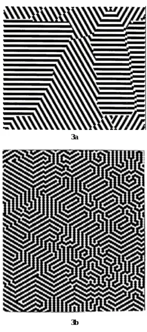
As a matter of fact, for magnetic materials with a strong perpendicular anisotropy, as bubble materials [38], this dipolar hexagonal symmetry shown in equations (7) and induced by lattice symmetry determines the direction of the 2D domain walls of the labyrinthine structure as observed both experimentally and numerically [47]. These walls are perpendicular to the dense axes of the film, i.e. parallel to the magnetization which is itself parallel to the easy magnetic axis. Such labyrinthine structures are reported in Figures 3a and 3b. The details observed in Figure 3a well evidence the three dominant directions while the large scale structure observed in Figure 3b confirms these dominant directions and shows the formation of parallel chevrons and of rather simple labyrinths in Monte-Carlo simulations at low temperature [7]. The large scale effect of Fig. 3b is once more due to the choice of a large dipole versus exchange ratio as explained before. Moreover a temperature increase induces a more complex labyrinthine structure as

3a

3b

Figure 3. Portions of Ising spin structures on triangular lattices. Black stripes, up

spins; white stripes, down spins. (a) 100x100 spins D/Ja3=0.75 and kT/J=0.1; (b) 200x200 spins J=0 and kT/D=0.05. In each Figure stripes occur along three directions.

already reported [7, 47]. Once more the close similarity between magnetic textures and liquid crystal textures must be noticed [48].

2.3. Higher order lattice sums

For these terms, lattice sums diverge. So these sums must be computed over finite samples and main contributions come from external layers. For such external parts, the lattice symmetry effect is quite lowered since in large rings a large number of sites act practically as in a continuum network. So an integral treatment of these sums is convenient, with the following results where radial and angular contributions are easily separated [33]:

q p q p q p A B I , = , , q p q p q p A B J , ,1,1= , +2, ₍₈₎ 1 , , 1 , 2 , , 2 , 1 , ,q = pq = pq pq+ p J A B J 2 , , 2 , 2 , ,q = pq pq+ p A B J

In the case of integration over a circular ring limited by an external circle of radius L and an internal circle of radius a, just one sort of radial integral A and one sort of angular integral B appear when describing all lattice sums I and J, they are:

) 1 ( ! ! ! ! 1 2 1 1 , _{+ −} − = = +− + − +−

∫

r dr L_{pq p} a_q q p A q p q p L a q p q p (9a)

∫

=2π θ θ θ 0 , cos sin d Bpq p q (9b)

Equation (9a) well shows divergence when p+q>1, and logarithmic divergence for p+q=1. So the strength of the corrective term when p+q>1 is well evidenced. Equation (9b) gives classical trigonometric integrals of which the first ones are reported in a short table in ref. 28. Finally these calculated integrals enable us to rewrite the dipolar Hamiltonian as a sum of local contributions of the spin field and its derivatives. Then the ground state determination is easily studied in a local Landau picture.

3. Ground state determination

3.1. Cartesian ground state equations

The local dipolar Hamiltonian is parted according to the level of derivation:

∑

= = à n n i i H H , (10)

Of course only the first terms are effectively relevant because of the corrective term. The first term Hi,0 is associated with anisotropy as seen

before. The next non zero term is the second one because of symmetry consideration. More generally there are only even values of n always because of symmetry. The second term reads when introducing the explicit values of the angular lattice sums:

y x S S y x S S y S S y S S x S S x S S A H x y y x y y x x y y x x _{∂ ∂} ∂ − ∂ ∂ ∂ − ∂ ∂ − ∂ ∂ + ∂ ∂ + ∂ ∂ − = 2 2 2 2 2 2 2 2 2 2 0 , 2 2 _{5 3 3 5 6 6} 4 π (11) Here A2,0 is positive as noticed from eq (9). By means of integration by parts this energy density reads as a quadratic function of the first order spin derivatives, when neglecting boundary terms:

⎟⎟ ⎠ ⎞ ⎜⎜ ⎝ ⎛ ∂ ∂ ⎟ ⎠ ⎞ ⎜ ⎝ ⎛ ∂ ∂ + ⎟⎟ ⎠ ⎞ ⎜⎜ ⎝ ⎛ ∂ ∂ + ⎟⎟ ⎠ ⎞ ⎜⎜ ⎝ ⎛ ∂ ∂ − ⎟⎟ ⎠ ⎞ ⎜⎜ ⎝ ⎛ ∂ ∂ − ⎟ ⎠ ⎞ ⎜ ⎝ ⎛ ∂ ∂ = y S x S y S y S x S x S A H x y x y x y 12 5 3 3 5 4 2 2 2 2 0 , 2 2 π (12)

This expression can be compared with the corresponding square of the magnetization gradient obtained for exchange [41] and shows the very anisotropic nature of dipolar interaction. This quadratic form of the energy density reads in matrix notation:

⎟ ⎟ ⎟ ⎟ ⎟ ⎟ ⎟ ⎟ ⎟ ⎟ ⎟ ⎠ ⎞ ⎜ ⎜ ⎜ ⎜ ⎜ ⎜ ⎜ ⎜ ⎜ ⎜ ⎜ ⎝ ⎛ ⎟⎟ ⎠ ⎞ ⎜⎜ ⎝ ⎛ ∂ ∂ ⎟⎟ ⎠ ⎞ ⎜⎜ ⎝ ⎛ ∂ ∂ ⎟⎟ ⎠ ⎞ ⎜⎜ ⎝ ⎛ ∂ ∂ ⎟ ⎠ ⎞ ⎜ ⎝ ⎛ ∂ ∂ ⎟⎟ ⎟ ⎟ ⎟ ⎠ ⎞ ⎜⎜ ⎜ ⎜ ⎜ ⎝ ⎛ − − ⎟⎟ ⎠ ⎞ ⎜⎜ ⎝ ⎛ ∂ ∂ ⎟⎟ ⎠ ⎞ ⎜⎜ ⎝ ⎛ ∂ ∂ ⎟⎟ ⎠ ⎞ ⎜⎜ ⎝ ⎛ ∂ ∂ ⎟ ⎠ ⎞ ⎜ ⎝ ⎛ ∂ ∂ ≈ y S x S y S x S y S x S y S x S H y y x x y y x x 5 0 0 6 0 3 0 0 0 0 3 0 6 0 0 5 2 (12a)

This term can be compared with the Oseen-Zöcher-Frank phenomenological equations for nematic liquid crystals [21]. It has four eigenvalues (11,−1,−3,−3). This also induces anisotropy.

The fourth term of the Hamiltonian is obtained from a similar calculation and reads up to a numerical factor:

⎟ ⎟ ⎠ ⎞ ⎜ ⎜ ⎝ ⎛ ∂ ∂ ∂ + ∂ ∂ ∂ − ⎟ ⎟ ⎠ ⎞ ⎜ ⎜ ⎝ ⎛ ∂ ∂ ∂ + ∂ ∂ ∂ − ∂ ∂ − ∂ ∂ + ∂ ∂ ∂ − ∂ ∂ ∂ − ∂ ∂ + ∂ ∂ − = 3 4 3 4 3 4 3 4 4 4 4 4 2 2 4 2 2 4 4 4 4 4 0 , 4 4 12 12 9 3 6 6 3 9 8 y x S y x S S y x S y x S S y S S y S S y x S S y x S S x S S x S S A H x x y y y x y y x x y y x x y y x x π (13) Here too this expression could be read as a quadratic function of partial derivatives of order two of the spin field, up to boundary terms, by means of integration by parts.

Because of the previous remark done on the anisotropic properties of

H0, for a system driven only by dipolar interactions the ground state local magnetization lies in the plane. So this local magnetization is

characterized at each site by the angle θ that the local spin makes with axis x'x: S=(cosθ,sinθ,0). So the ground state research is just the search for the optimal angular function θ

( )

x,y . And the constraints of the level-two local Hamiltonian, i.e. of the level-two energy density, are for this

function:

(

)

2 2

(

2 2

)

2 4sin2 x2 y2 6cos2 xy x x 6sin2 x y 4cos2 x x

H ≈ θθ −θ − θθ +θ +θ + θθ θ + θθ −θ

(14)

This expression is obviously non linear. The original dipolar interaction is bilinear and non local [34]. So when translated into a local interaction, equation (14) means it becomes a non linear local interaction.

And at level four these constraints are, after an easy but tedious calculation:

(

)

(

) (

)

(

)

(

)

(

)

(

)

[

]

(

)

[

]

(

)

2

(

)

(

)

2 2 4 2 2 4 2 2 2 2 2 2 4 2 12 12 4 2 4 3 4 1 sin 4 3 4 1 cos 4 2 cos 4 2 6 6 2 3 3 4 2 2 sin 2 2 2 2 2 2 2 2 2 2 3 2 3 3 3 2 2 2 2 2 2 4 3 4 4 y x y x y x y x xy xy y x x xy y y x y y y y x x x x xy y x y x y x y y x x x y y x y x y x xy x y y x y x H θ θ θ θ θ θ θ θ θ θ θ θ θ θ θ θ θ θ θ θ θ θ θ θ θ θ θ θ θ θ θ θ θ θ θ θ θ θ θ θ θ θ θ θ θ θ θ θ θ θ θ − + − + − + + + + − + − + − + − + + − ⎥ ⎥ ⎦ ⎤ ⎢ ⎢ ⎣ ⎡ + − − + + + − + + + + − ≈ (15)

Again a strong non linearity makes the ground state resolution so complex. Of course a complete resolution would determine this function

( )

x,y

θ from boundary conditions. It would be a quite uneasy task. Here we will just compare solutions which are suggested by experimental observation as realistic ones. And for vortex as well as hyperbolic solutions as observed numerically and experimentally a polar representation is quite useful.

3.2. Polar ground state equations at order 2

Central vortices appear in numerical simulations [7] and well agree with experimental observations [2, 4]. They are easily described in polar coordinates

( )

r,ϕ according to their chirality by:

( )

π π ϕ θ 2 2 ± = (16) Quite similarly hyperbolic topological defects with two sorts of chirality appear numerically and experimentally. They are defined by:

( )

π π ϕ θ 2 2 ± − = (17) These topological defects are characterized from their field lines with:

(

θ ϕ

)

ϕ = cot −

rd dr

In this case these field lines are either circles around the origin or hyperbolas such as r cos2ϕ =C.

Figure 4 exhibits vortices and a hyperbolic topological defect. In these expressions the choice of the free sign corresponds to the choice of the vortex or hyperbolic defect chirality. Of course the interest in such structures starts from their natural observation in low temperature simulations as noticed in Figure 2 where both defects appear. It must be noticed that the nearest neighbours of a vortex are hyperbolic defects or higher order defects and reciprocally, with shorter minimal distances for vortex-hyperbola than for vortex-vortex or for hyperbola-hyperbola. These defects also appear in the experimental observation in 2D magnets [15, 39] as well as in liquid crystals [43-45]. The part of these defects appears in the level two Hamiltonian expressed in polar coordinates while higher order defects appear in further expansion steps. So this gives rise to a natural classification of topological defects according to the level of appearance in the local dipolar Hamiltonian.

a

b c

Figure 4. Principle of topological defects: (a) vortex with positive chirality; (b) vortex

with negative chirality; (c) hyperbolic defect with negative chirality.

As obvious from Figure 4 polar coordinates are introduced. This is done by the use of the transformation of the function θ

( )

x,y which becomes a function

( )

ϕ

θ r, of polar coordinates. Derivatives at all order follow with at first order:

r y r x r r ϕθ θ ϕ θ ϕθ θ ϕ θ ϕ ϕ sin cos cos sin + = + − = (18)

The other derivatives are easily deduced. It enables us to rewrite the previous energy density at different levels as functions of θ

( )

r,ϕ and its derivatives.

The energy density at level two reads:

( )

[

]

[

( )

]

_{

_[

_{( )}

_]

_[

_{( )}

_]

_} ( )

[

]

[

( )

]

{ ϕ θ ϕ θ } θ {

[

(ϕ θ)

]

[

(ϕ θ)

]

} θ θ ϕ θ ϕ θ θ θ θ θ θ ϕ θ ϕ ϕ ϕ ϕ ϕ − + + + + − − + − + − − + + ⎟ ⎟ ⎠ ⎞ ⎜ ⎜ ⎝ ⎛ − + + − − ≈ 2 cos 7 2 cos 2 2 2 cos 7 2 cos 2 2 2 cos 7 2 cos 2 2 2 sin 2 sin 7 2 2 2 2 0 , 2 2 2 2 r r r r r r r A H (19) This expression evidences the part of vortices and hyperbolic defects as described by equations (16). This evidence fully justifies the introduction of

polar coordinates. When testing the validity of a vortex or hyperbolic defect solution, the only non zero derivative is obviously:

1 ± = ϕ

θ

Using this remark the energy density at level two becomes:

(

)

[

]

[

(

)

]

{

ϕ θ ϕ θ

}

θϕ _{− + − −} ≈ 2 cos2 7cos2 2 2 2 0 , 2 2 r A H (19)

This energy density shows a modulated maximum for the vortices described by θ ϕ π

( )

2π

2 ±

= and a positive modulated local minimum for the

hyperbolic defects described by θ ϕ π

( )

2π 2 ± −

= . Since the energy density

of this modulated minimum is positive, it is higher than that of a simple ferromagnetic state θ=const. So these vortices states would be metastable if there was no corrective term in the energy density. But, as noticed before, the energy density corrective terms are of the same order as the energy density at level two, so vortices can be stable.

The first conclusions which come from this calculation are:

- There is evidence for vortices and hyperbolic defects as well defined states as seen in Eqs (18) and (19).

- The stability of vortex and other defects arrangements must be studied carefully from a Hamiltonian which does not describe dipole-dipole interaction but deals with effective vortex-dipole interactions or hyperbolic defect-dipole interactions or vortex-vortex interactions since multipolar interactions are obviously more screened than simple dipole-dipole interactions. These multipole-dipole-dipole or multipole-multipole interactions are more localized, being driven by a larger radial exponent. Thus lattice sums show a better convergence in that case than for dipole-dipole interaction. The total moment of a vortex or of a hyperbolic defect is zero, so the first non zero terms are due to higher cumulants than for dipole-dipole interaction. This shift of the effective interaction towards higher order terms increases the convergence of multipole interaction lattice sums. So these effective interactions involve more numerous convergent lattice sums and thus lead to a better optimization process. These effective defect-defect interactions will allow us to calculate the energy density at level two at least, with the possibility of neglecting the

corrective term, i.e. in a safe condition, but at the price of the introduction of numerous new interactions according to the defect natures and sizes.

These convergence problems can be further optimized in several ways and steps as noticed quite earlier by Ewald [49] when using Fourier transforms about infinite dipole lattice sums. A second step of the interaction screening consists in introducing pairs of vortices or pairs of hyperbolic defects of opposite chirality, or mixed pairs of defects. As a result it will introduce more convergent lattice sums. And so the spatial extension of vortices and hyperbolic defects could be optimized.

However, pairs of vortices of opposite chirality or pairs of defects introduce anisotropy as defining the starting point of a line of vortex or of defects, as it occurs in a Von Karman alley in hydrodynamics. So a third step in improving the magnetic screening of the dipolar interaction consists in introducing a real two dimensional problem. There are at least two ways of introducing dimensionality two:

- introducing two orthogonal pairs of vortices, a vortex square, - or introducing three pairs of vortex, a vortex hexagon.

And a vortex square introduces a hyperbolic defect in its centre while a vortex hexagon introduces higher order defects in its centre.

Clearly these considerations introduce a multipolar screening which will enable us to derive the full stability picture at the price of heavy work. For instance a next crown of vortex around the square or hexagon can be chosen in order to increase the screening, with the introduction of square or triangular symmetry for comparison. In this case other topological defects such as hyperbolic ones are also implied as seen on Figure 2. So discrete screening is a very difficult problem. Moreover there is no theoretical evidence for a simple final configuration as well as there is no general experimental evidence for that. Of course the occurrence of boundary conditions and impurities increases this complexity.

3.3. Polar ground state equations at order 4

The calculation of the energy density at level four is instructive since it reveals once more the nature of these terms, even if this analysis remains here rather academic because of non negligible corrective term. So we just write the contribution to the energy density at level four which depends only on the partial first order angular derivative θ_ϕ and its powers, in order to observe the effect on vortices and other topological defects with radial invariance:

(

)

[

]

[

(

)

]

{

}

(

)

[

]

[

(

)

]

( )

{

}

(

)

[

]

[

(

)

]

(

)

(

)

( )

{

}

(

)

[

]

[

(

)

]

( )

(

)

{

θ ϕ θ ϕ ϕ ϕ θ ϕ θ

}

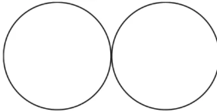
θ ϕ θ ϕ θ ϕ ϕ θ ϕ θ θ ϕ ϕ θ ϕ θ θ ϕ θ ϕ θ θ ϕ ϕ ϕ ϕ 2 4 2 4 2 4 3 2 4 0 , 4 4 sin cos cos sin 2 sin 5 . 1 2 cos 2 cos 1 2 cos 12 2 4 cos 2 4 cos 2 cos 6 2 cos 16 4 cos 11 2 cos 26 2 cos 46 13 2 cos 2 2 cos 6 + − − + − − + + + + + − − + − − + + + + − + + + − − − ≈ r A H (20) This result well exhibits the part of the two defects vortex and hyperbolic defects, and it introduces other topological defects as well as a quartic modulation. The new topological defects are:

) ( 2ϕ π θ = _(21a) ) ( 2 2ϕ π π θ= + (21b) ) ( 2ϕ π θ =− _(21c) ) ( 2 2ϕ π π θ=− + (21d)

They define four field lines parallel to the magnetization

(

θ ϕ

)

ϕ = cot −

rd dr

, respectively a double circle and a sextic curve

3 / 1 0 cos3ϕ

r

r= with sixfold symmetry and six asymptots. Such a double

circle is observed in micromagnetic simulations [50] and parts of the sextic curve are present in Figure 2. Figure 5 shows the double circle

Quite obviously the next step will introduce new defects and a modulation of order six. These new defects are characterized by the equations:

( )

π ϕ

θ=±3 2 (22)

And in Cartesian coordinates, the quartic curves:

(

x2 +y2

)

2 −a2

(

x2 −y2

)

=0 (22a) 0 6 2 2 4 4 4_{− + − =} a y y x x (22b)

And extrapolation to next orders gives a complete series of defects with

( )

π

ϕ

θ=±n 2 ₍₂₃₎

In polar coordinates, there are algebraic curves

(

)

[

1ϕ

]

( )

2π cos 1 0 1₌ − ₋ − n r rn n (23a)

(

)

[

1ϕ

]

( )

2π cos 1 0 1₌ −− ₊ − − _{r n} r n n

One recognizes here Frank’s disclinations in liquid crystals with integer values of

n [44], while for liquid crystals half integer values of n are admitted. This

specificity of liquid crystals is due to the lower symmetry of liquid crystals where the order parameter is just a direction, while for magnetic materials, the order parameter is the spin, a real vector. So the number of magnetic topological defects is reduced in front of the number of liquid crystals topological defects. There is already evidence for such a series of such 2D topological defects with numerous asymptotic branches in magnetic simulations [7], in experiments [47] as well in observation of liquid crystals [39].

3.4. The first four topological defects and their effective potentials

As already introduced in equations (16) and (17) and in Figure 4, the first topological defects to appear are two vortices and two hyperbolas. The simplest view of these defects is reported in Figure 6 on a square lattice.

These defects are known as classical signs. The two vortices are usually called swastika from early Indian language. The two hyperbolas can be deduced from each other by a 90° rotation and appear as a mouth, or a frank ax when rotated by 45°. Their interaction potential with a spin are easily calculated when their centres are at the origin. They are for a lattice parameter a and a unit value of the spin, at first non negligible order:

V1 V2 H1 H2

Figure 6. The four basic topological defects: vortex1 (V1), vortex2 (V2), hyperbolic

defect 1 (H1) and hyperbolic defect 2 (H2).

For V1: _V

(

_{y x}

)

(

OM s

)

_z R a ys xs R a U 1= ₅ − = ₅ ∧ 6 6 ₍₂₄₎ For H1:

[

(

2 2

)

(

2 2

)

]

7 1 9 9 6 y x ys y x xs R a UH = y − + x − + (25)

These interactions are of higher order than the dipole-dipole interaction since the sum of these interacting dipoles is zero. The vortex dipole interaction evidences a chiral effect while the hyperbola-spin interaction is a little bit more complex. Since vortices 1 and 2 have opposite interactions as well as hyperbolas 1 and 2, the association of two vortex of opposite chirality as well as the association of orthogonal hyperbolas leads to a higher order interaction. The association vortex-hyperbola does not increase the interaction level.

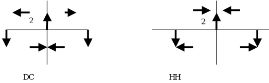
3.5. The main second topological defects

As just written the main second topological defects are the associations of opposite topological defects, i.e. V1V2 or H1H2. Of course there are

different geometrical associations, and there are just two simplest such defects up to rotations, namely the double circle and the sextic curve

already introduced. This is shown in Figure 7 where such associations are reported.

Of course, the order of associated defects as well as the direction defined by associated defects can be changed so finally eight distinct second order topological defects are introduced. As noticed before, they appear in the Hamiltonian and are observed in micromagnetism calculations. The effective interaction created by two vortices of opposite chirality and distant from 2d on the axis x’x is, with a left anticlockwise vortex and a right clockwise vortex, more localized interaction than vortex-spin interaction, as expected. Its symmetry is well noticed. So the fields created by a square of vortices and by a hexagon of vortices can be easily deduced.

DC HH

2 2

Figure 7. The two second order topological defects: DC the double circle and HH the

sextic curve.

Of course higher order defects can be added and they evidence the progressive screening of the dipolar interaction.

4. Defect dynamics and conclusions

The previous determination of the local dipolar Hamiltonian is quite useful to classify intrinsic defect dynamics from this energy landscape, even if the inertial part which can be calculated as a Döring’s mass [51] is less obvious. A first natural motion comes from the defect centre motion. This is not a simple motion since it must compete with other defect motions within the sample. A second mode corresponds to the radial “breathing” mode which consists in an increase and decrease of the defect size. Of course such magnetic breathing and shrinking modes must also be conjugated over several defects for a given sample. From equation (20) and its quartic modulation, quartic deformations of these topological defects also occur. This defines a third series of modes. The extrapolation to higher order of the local Hamiltonian shows other modulations of higher symmetry such as sixfold, eightfold and so on. Moreover these extrapolations show the appearance of new topological defects as double circle and sextic defect which can be created or annihilated, a fourth series of modes. Since the spatial extension of such defects is quite low as observed in Figure 2, their creation or annihilation must have a rather low eigen frequency, and these modes are expected to be rather independent from the rest of the sample. So many new modes appear. Because of their different symmetry they are submitted to different selection rules which can be used to select them in resonance experiments. Since these numerous modes are more or less localized, their interaction with external fields can also be distinguished. These two points suggest a lot of different experimental observations of these modes.

The general analysis of defect stability can be easily derived from the transposition of equations (19) and (20) to the case of a screened interaction, where screening is due to a more complex structure at the origin. Then the resulting energy density for this defect reads because of the competition between successive even orders in the interaction, when omitting extra modulations: ⎟ ⎠ ⎞ ⎜ ⎝ ⎛ ₋ − ⎟ ⎠ ⎞ ⎜ ⎝ ⎛ ₋ = 1_n 1_{n n}1_{−2 n}1₋₂ a L B a L A H (27) In equations (19) and (20) the parameter values A and B are positive, and we admit this here.

So a natural defect length appears:λ=

[

nA

(

n−2 B

)

]

12. If this natural defect length λ _{is larger than the inner integration radius a of lattice sums,} then the defect is stable as compared with the ferromagnetic arrangement when the lateral sample radius L is smaller than the value L1 which satisfies the equation: ⎟ ⎟ ⎠ ⎞ ⎜ ⎜ ⎝ ⎛ − − ⎟ ⎟ ⎠ ⎞ ⎜ ⎜ ⎝ ⎛ − = _{−2 −2} 1 1 1 1 1 1 0 _{n n n n} a L B a L A (28)

If the sample is larger than this disk of radius L1, the one defect situation is no longer stable in front of the ferromagnetic arrangement. So, probably different defects of different species appear simultaneously in the sample in order to obtain a stable solution as observed in large samples [38].

If the natural defect length λ is smaller than the inner integration radius

a, then the defect is never stable. This situation seems to be never observed.

So the practical conclusion is that a one vortex configuration is stable up to some limiting sample lateral size. For larger samples more complex configurations are expected. This well agrees with observation at a larger scale [36, 47].

About defect dynamics, the previous remarks show the abundance of excitation modes which can be selected according to selection rules when using convenient excitation fields, i.e. magnetic fields with convenient symmetry.

Finally this hierarchy of more and more localized defects called disclinations for liquid crystals and the induced hierarchy of their well defined excitation modes could be used to introduce highly localized memory units with a well controlled production and reading [36].

References

1. A. Vaterlaus, C. Stamm, U. Maier, M. G. Pini, P. Politi and D. Pescia, Phys. Rev. Lett. 84, 2247 (2000).

2. S. P. Li, D. Peyrade, M. Natali, A. Lebib, Y. Chen, U. Ebels, L. D. Buda, K. Ounadjela, Phys. Rev. Lett. 86, 1102 (2001); S. P. Li, M. Natali, A. Lebib, A. Pépin, Y. Chen, Y. B. Xu, J. Magn. Magn. Mat. 241, 447 (2002).

3. T. Shinjo, T. Okuno, R. Hassdorf, K. Shigeto, T. Ono, Science 289, 930 (2000). 4. T. Duden and E. Bauer, Phys. Rev. Lett. 77, 2308 (1996); M. Hehn, R. Ferre, K.

Ounadjela, J.-P. Bucher and F. Rousseaux, J. Magn. Magn. Mater. 165, 5 (1997). 5. R. P. Cowburn * and M. E. Welland, Phys. Rev. B 58, 9217 (1998).

6. A.B. MacIsaac, J.P. Whitehead, K. De’Bell and P.H. Poole, Phys. Rev. Lett. 77, 739 (1996); A.B. MacIsaac, K. De’Bell and J.P. Whitehead, Phys. Rev. Lett. 80, 616 (1998); A. Hucht, A. Moschel and K.D. Usadel, J. Magn. Magn. Mater. 148, 32 (1995);

7. P.I. Belobrov, V.A. Voevodin and V.A. Ignatchenko, Sov. Phys. JETP 61, 522 (1985); E.Y. Vedmedenko, A. Ghazali and J.-C.S. Levy, Surf. Sci. 402-404, 391 (1998); Phys. Rev. B 59, 3329 (1999); E.Y. Vedmedenko, H.P. Oepen, A. Ghazali, J.-C.S. Levy and J. Kirschner, Phys. Rev. Lett. 84, 5884 (2000); J. Sasaki and F. Matsubara, J. Phys. Soc. Japan 66, 2138 (1997).

8. J.-G. Zhu and H.N. Bertram, J. Appl. Phys. 63, 3248 (1988); I.R. McFadyen and I.A. Beardsley, J. Appl. Phys. 67, 5540 (1990).

9. D.R. Fredkin and T.R. Koehler, J. Appl. Phys. 67, 5544 (1990); D.R. Fredkin, T.R. Koehler, J.F. Smyth and S. Schultz, J. Appl. Phys. 69, 5276 (1991). 10. S. Rohart, V. Repain, A. Thiaville, and S. Rousset, Phys. Rev. B 76, 104401 (2007). 11. Ph. Depondt and F. Mertens, private communication.

12. J.N. Chapman, J. Phys. D 17, 623 (1984).

13. A.C. Daykin and J.P. Jakubovics, J. Appl. Phys. 80, 3408 (1996).

14. K. Koike and K. Hayakawa, Jpn. J. Appl. Phys. Part 2, 23 L187 (1984); H.P. Oepen, G. Steierl and J. Kirschner, J. Vac. Sci. Technol. B 20, 2535 (2002). 15. J. Li and C. Rau, Phys. Rev. Lett. 97, 107201 (2006) ; J.E. Villegas, C.-P. Li and

I.K. Schuller, Phys. Rev. Lett. 99, 227001 (2007) .

16. K.-S. Lee, K.Y. Guslienko, J-Y. Lee and S.-K. Kim, Phys. Rev. B 76, 174410 (2007); J.-G. Caputo, Y. Gaididei, V.P. Kravchuk, F.G. Mertens and D.D. Sheka, Phys. Rev. B 76, 174428 (2007) ; J-Y. Lee, K.-S. S. Choi Lee, K.Y. Guslienko, and S.-K. Kim, Phys. Rev. B 76, 184408 (2007).

17. N.D. Mermin, H. Wagner, Phys. Rev. Lett. 17, 1133 (1966); B. Jancovici, Phys. Rev. Lett. 19, 20 (1967).

18. J.M. Kosterlitz and D.J. Thouless, J. Phys. C 6, 1181 (1973); B.I. Halperin and D.R. Nelson, Phys. Rev. Lett. 41, 121 (1978); A.P. Young, Phys. Rev. B 19, 1855 (1979). 19. Y. Yafet and E.M. Gyorgy, Phys. Rev. B 38, 9145 (1988).

20. F.C. Frank, Disc. Faraday Soc. 25, 19 (1958).

21. for a review see: P.G. de Gennes and J. Prost, “The Physics of Liquid Crystals” Oxford Clarendon Press (1993); S. Chandrasekhar, “Liquid Crystals” Cambridge University Press, Cambridge (1992).

22. E.Y. Vedmedenko, H.P. Oepen and J. Kirschner, Phys. Rev. B 66, 214401 (2002); Phys. Rev. B 67, 012409 (2003).

23. E.Y. Vedmedenko, H.P. Oepen and J. Kirschner, J. Magn. Magn. Mater. 256, 237 (2003).

24. A. Montanari and G. Semerjian, Phys. Rev. Lett. 94, 247201 (2005).

25. L. Del Bianco, A. Hernando, A. Multigner, C. Prados, J.C. Sanchez-Lopez, A. Fernandez, C.F. Conde and A. Conde, J. Appl. Phys. 84, 2189 (1998).

26. E. O. Kamenetskii, Michael Sigalov, and Reuven Shavit, Phys. Rev. E 74, 036620 (2006); T. Shinjo, T. Okuno, R. Hassdorf, K. Shigeto, and T. Ono

Science 289, 930 (2000).

27. G.R. Berdiyorov, M.V. Milosevic and FM. Peeters, Phys. Rev. B 74, 174512 (2006).

28. Z. Zhang, P.C. Hammel and P.E. Wigen, Appl. Phys. Lett. 68, 2005 (1996). 29. J.P. Park, P. Eames, D.M. Engebretson, J. Berezovsky and P.A. Crowell, Phys.

Rev. Lett. 89, 277201 (2003).

30. M. Bailleul, D. Olligs and C. Fermon, Phys. Rev. Lett. 91, 137204 (2003). 31. G. Gubbiotti, C. Carlotti, T. Okuno, T. Shinjo, F. Nizzoli and R. Zivieri, Phys.

Rev. B 68, 184409 (2003).

32. R. L. Compton and P. A. Crowell, Phys. Rev. Lett. 97, 137202 (2006). 33. J.-C.S. Levy, Phys. Rev. B 63, 104409 (2001).

34. L. D. Landau and E.M. Lifshitz, “The classical theory of fields” 2nd edition, Pergamon Press, Oxford (1962),p. 119.

35. R. Allenspach and A. Bischof, Phys. Rev. Lett. 69, 3385 (1992).

36. R. Zdyb, A. Pavloska, A. Locatelli, S. Heun, S. Cherifi, R. Belkhou and E. Bauer, Appl. Surf. Sci. 249, 38 (2005).

37. A.B. Johnston, J.N. Chapman, B. Khamsehpour and C.D.W. Wilkinson, J. Phys. D: Appl. Phys. 29, 1419 (1996); R. Ferré, M. Hehn and K. Ounadjela, , J. Magn. Magn. Mater. 165, 9 (1997).

38. A. H. Bobeck and E. Della Torre, “Magnetic Bubbles” NHPC, Amsterdam 1975. 39. A. Hubert and R. Schaefer, “Magnetic Domains” (Springer, Berlin 1998). 40. I. Booth, A.B. MacIsaac, J.P. Whitehead and K. De’Bell, Phys. Rev. Lett. 75, 950

(1995); K. De’Bell, A.B. MacIsaac and J.P. Whitehead, Rev. Mod. Phys. 72, 225 (2000); O. Iglesias and A. Labarta, J. Magn. Magn. Mater. 221, 149 (2000). 41. J.A. Cape and G.W. Leman, J. Appl. Phys. 42, 5732 (1971); T. Garel and S.

Doniach, Phys. Rev. B 26, 325 (1982).

42. J.I. Martin, J. Nogués, Kai Liu, J.L. Vicent and Ivan K. Schuller, J. Magn. Magn. Mater. 256, 449 (2003).

43. H.E. Assender and A.H. Windle, Polymer, 38, 677 (1997); T. C. Lubensky, David Pettey, Nathan Currier, and Holger Stark, Phys. Rev. E 57, 610 (1998). 44. C. Robinson, J.C. Ward and R.B. Beevers, Disc. Faraday Soc. 25, 29 (1958). 45. M. Kleman and O.D. Lavrentovitch, Philos. Mag. 86, 4117 (2006).

46. M. Ye, Y. Yokoyama and S. Soto, Appl. Phys. Lett. 89, 141112 (2006).

47. P. Molho, J.L. Porteseil, Y. Souche, J. Gouzerh and J.-C.S. Levy, J. Appl. Phys.

61, 4188 (1987); G.S. Kandaurova, A.E. Sviderskiy, V.P. Klin and V.I. Chany, J.

48. M. Seul and D. Anderman, Science, 267, 476 (1995).

49. M.P. Allen and D. J. Tildesley, “Computer Simulation of Liquids” Oxford: Clarendon Press (1989).

50. W. Schepper, H. Kubota and G. Reiss, in “Nanostructured Magnetic Materials and their Aplications” eds. D. Shi, B. Aktas, L. Pust and F. Mikailov, Springer, Berlin (2002) p. 91.