HAL Id: hal-00271141
https://hal.archives-ouvertes.fr/hal-00271141
Submitted on 21 Jan 2010
HAL is a multi-disciplinary open access
archive for the deposit and dissemination of
sci-entific research documents, whether they are
pub-lished or not. The documents may come from
teaching and research institutions in France or
abroad, or from public or private research centers.
L’archive ouverte pluridisciplinaire HAL, est
destinée au dépôt et à la diffusion de documents
scientifiques de niveau recherche, publiés ou non,
émanant des établissements d’enseignement et de
recherche français ou étrangers, des laboratoires
publics ou privés.
A review of image denoising algorithms, with a new one
Antoni Buades, Bartomeu Coll, Jean-Michel Morel
To cite this version:
Antoni Buades, Bartomeu Coll, Jean-Michel Morel. A review of image denoising algorithms, with
a new one. Multiscale Modeling and Simulation: A SIAM Interdisciplinary Journal, Society for
Industrial and Applied Mathematics, 2005, 4 (2), pp.490-530. �hal-00271141�
ONE.
A. BUADES † ‡, B. COLL †, AND J.M. MOREL ‡
Abstract. The search for efficient image denoising methods still is a valid challenge, at the crossing of functional analysis and statistics. In spite of the sophistication of the recently proposed methods, most algorithms have not yet attained a desirable level of applicability. All show an out-standing performance when the image model corresponds to the algorithm assumptions, but fail in general and create artifacts or remove image fine structures. The main focus of this paper is, first, to define a general mathematical and experimental methodology to compare and classify classical image denoising algorithms, second, to propose an algorithm (Non Local Means) addressing the preservation of structure in a digital image. The mathematical analysis is based on the analysis of the “method noise”, defined as the difference between a digital image and its denoised version. The NL-means algorithm is proven to be asymptotically optimal under a generic statistical image model. The de-noising performance of all considered methods are compared in four ways; mathematical: asymptotic order of magnitude of the method noise under regularity assumptions; perceptual-mathematical: the algorithms artifacts and their explanation as a violation of the image model; quantitative experi-mental: by tables of L2 distances of the denoised version to the original image. The most powerful
evaluation method seems, however, to be the visualization of the method noise on natural images. The more this method noise looks like a real white noise, the better the method.
Key words. Image restoration, non parametric estimation, PDE smoothing filters, adaptive filters, frequency domain filters
AMS subject classifications. 62H35
1. Introduction.
1.1. Digital images and noise. The need for efficient image restoration meth-ods has grown with the massive production of digital images and movies of all kinds, often taken in poor conditions. No matter how good cameras are, an image improve-ment is always desirable to extend their range of action.
A digital image is generally encoded as a matrix of grey level or color values. In the case of a movie, this matrix has three dimensions, the third one corresponding to time. Each pair (i, u(i)) where u(i) is the value at i is called pixel, for “picture element”. In the case of grey level images, i is a point on a 2D grid and u(i) is a real value. In the case of classical color images, u(i) is a triplet of values for the red, green and blue components. All of what we shall say applies identically to movies, 3D images and color or multispectral images. For a sake of simplicity in notation and display of experiments, we shall here be contented with rectangular 2D grey-level images.
The two main limitations in image accuracy are categorized as blur and noise. Blur is intrinsic to image acquisition systems, as digital images have a finite number of samples and must satisfy the Shannon-Nyquist sampling conditions [32]. The second main image perturbation is noise.
†Universitat de les Illes Balears, Anselm Turmeda, Ctra. Valldemossa Km. 7.5, 07122 Palma de
Mallorca, Spain. Author financed by the Ministerio de Ciencia y Tecnologia under grant TIC2002-02172. During this work, the first author had a fellowship of the Govern de les Illes Balears for the realization of his PhD.
‡Centre de Mathmatiques et Leurs Applications. ENS Cachan 61, Av du Prsident Wilson 94235
Cachan, France. Author financed by the Centre National d’Etudes Spatiales (CNES), the Office of Naval Research under grant N00014-97-1-0839, the Direction Gnrale des Armements (DGA), the Ministre de la Recherche et de la Technologie.
Each one of the pixel values u(i) is the result of a light intensity measurement, usually made by a CCD matrix coupled with a light focusing system. Each captor of the CCD is roughly a square in which the number of incoming photons is being counted for a fixed period corresponding to the obturation time. When the light source is constant, the number of photons received by each pixel fluctuates around its average in accordance with the central limit theorem. In other terms one can expect fluctuations of order√n for n incoming photons. In addition, each captor, if not adequately cooled, receives heat spurious photons. The resulting perturbation is usually called “obscurity noise”. In a first rough approximation one can write
v(i) = u(i) + n(i),
where i ∈ I, v(i) is the observed value, u(i) would be the “true” value at pixel i, namely the one which would be observed by averaging the photon counting on a long period of time, and n(i) is the noise perturbation. As indicated, the amount of noise is signal-dependent, that is n(i) is larger when u(i) is larger. In noise models, the normalized values of n(i) and n(j) at different pixels are assumed to be independent random variables and one talks about “white noise”.
1.2. Signal and noise ratios. A good quality photograph (for visual inspec-tion) has about 256 grey level values, where 0 represents black and 255 represents white. Measuring the amount of noise by its standard deviation, σ(n), one can define the signal noise ratio (SNR) as
SN R = σ(u) σ(n),
where σ(u) denotes the empirical standard deviation of u,
σ(u) = Ã 1 |I| X i∈I (u(i)− u)2 !12 and u = 1 |I| P
i∈Iu(i) is the average grey level value. The standard deviation of the
noise can also be obtained as an empirical measurement or formally computed when the noise model and parameters are known. A good quality image has a standard deviation of about 60.
The best way to test the effect of noise on a standard digital image is to add a gaussian white noise, in which case n(i) are i.i.d. gaussian real variables. When σ(n) = 3, no visible alteration is usually observed. Thus, a 60
3 ≃ 20 signal to noise
ratio is nearly invisible. Surprisingly enough, one can add white noise up to a 2 1
ratio and still see everything in a picture ! This fact is illustrated in Figure 1.1 and constitutes a major enigma of human vision. It justifies the many attempts to define convincing denoising algorithms. As we shall see, the results have been rather deceptive. Denoising algorithms see no difference between small details and noise, and therefore remove them. In many cases, they create new distortions and the researchers are so much used to them as to have created a taxonomy of denoising artifacts: “ringing”, “blur”, “staircase effect”, “checkerboard effect”, “wavelet outliers”, etc.
This fact is not quite a surprise. Indeed, to the best of our knowledge, all denoising algorithms are based on
• a noise model
Fig. 1.1. A digital image with standard deviation 55, the same with noise added (standard deviation 3), the signal noise ratio being therefore equal to 18, and the same with signal noise ratio slightly larger than 2. In this second image, no alteration is visible. In the third, a conspicuous noise with standard deviation 25 has been added but, surprisingly enough, all details of the original image still are visible.
In experimental settings, the noise model is perfectly precise. So the weak point of the algorithms is the inadequacy of the image model. All of the methods assume that the noise is oscillatory, and that the image is smooth, or piecewise smooth. So they try to separate the smooth or patchy part (the image) from the oscillatory one. Actually, many fine structures in images are as oscillatory as noise is; conversely, white noise has low frequencies and therefore smooth components. Thus a separation method based on smoothness arguments only is hazardous.
1.3. The “method noise”. All denoising methods depend on a filtering pa-rameter h. This papa-rameter measures the degree of filtering applied to the image. For most methods, the parameter h depends on an estimation of the noise variance σ2.
One can define the result of a denoising method Dh as a decomposition of any image
v as
v = Dhv + n(Dh, v),
(1.1) where
1. Dhv is more smooth than v
2. n(Dh, v) is the noise guessed by the method.
Now, it is not enough to smooth v to ensure that n(Dh, v) will look like a noise.
The more recent methods are actually not contented with a smoothing, but try to recover lost information in n(Dh, v) [19], [25]. So the focus is on n(Dh, v).
Definition 1.1 (Method noise). Let u be a (not necessarily noisy) image and Dh a denoising operator depending on h. Then we define the method noise of u as
the image difference
n(Dh, u) = u− Dh(u).
(1.2)
This method noise should be as similar to a white noise as possible. In addition, since we would like the original image u not to be altered by denoising methods, the method noise should be as small as possible for the functions with the right regularity. According to the preceding discussion, four criteria can and will be taken into account in the comparison of denoising methods:
• a formal computation of the method noise on smooth images, evaluating how small it is in accordance with image local smoothness.
• a comparative display of the method noise of each method on real images with σ = 2.5. We mentioned that a noise standard deviation smaller than 3 is subliminal and it is expected that most digitization methods allow themselves this kind of noise.
• a classical comparison receipt based on noise simulation : it consists of taking a good quality image, add gaussian white noise with known σ and then com-pute the best image recovered from the noisy one by each method. A table of L2 distances from the restored to the original can be established. The L2
distance does not provide a good quality assessment. However, it reflects well the relative performances of algorithms.
On top of this, in two cases, a proof of asymptotic recovery of the image can be obtained by statistical arguments.
1.4. Which methods to compare ?. We had to make a selection of the de-noising methods we wished to compare. Here a difficulty arises, as most original methods have caused an abundant literature proposing many improvements. So we tried to get the best available version, but keeping the simple and genuine character of the original method : no hybrid method. So we shall analyze :
1. the Gaussian smoothing model (Gabor [16]), where the smoothness of u is measured by the Dirichlet integralR |Du|2;
2. the anisotropic filtering model (Perona-Malik [28], Alvarez et al. [1]); 3. the Rudin-Osher-Fatemi [31] total variation model and two recently proposed
iterated total variation refinements [36, 25];
4. the Yaroslavsky ([42], [40]) neighborhood filters and an elegant variant, the SUSAN filter (Smith and Brady) [34];
5. the Wiener local empirical filter as implemented by Yaroslavsky [40]; 6. the translation invariant wavelet thresholding [8], a simple and performing
variant of the wavelet thresholding [10];
7. DUDE, the discrete universal denoiser [24] and the UINTA, Unsupervised Information-Theoretic, Adaptive Filtering [3], two very recent new approaches; 8. the non local means (NL-means) algorithm, which we introduce here. This last algorithm is given by a simple closed formula. Let u be defined in a bounded domain Ω⊂ R2, then N L(u)(x) = 1 C(x) Z e−(Ga∗|u(x +.)−u(y+.)|2 )(0) h2 u(y) dy,
where x ∈ Ω, Ga is a Gaussian kernel of standard deviation a, h acts as a filtering
parameter and C(x) =R e−(Ga∗|u(x+.)−u(h2 z+.)|2 )(0)dz is the normalizing factor. In order
to make clear the previous definition, we recall that (Ga∗ |u(x + .) − u(y + .)|2)(0) =
Z
R2
Ga(t)|u(x + t) − u(y + t)|2dt.
This amounts to say that N L(u)(x), the denoised value at x, is a mean of the values of all pixels whose gaussian neighborhood looks like the neighborhood of x.
1.5. What is left. We do not draw into comparison the hybrid methods, in particular the total variation + wavelets ([7], [11], [17]). Such methods are significant improvements of the simple methods but are impossible to draw into a benchmark :
their efficiency depends a lot upon the choice of wavelet dictionaries and the kind of image.
Second, we do not draw into the comparison the method introduced recently by Y. Meyer [22], whose aim it is to decompose the image into a BV part and a texture part (the so called u + v methods), and even into three terms, namely u + v + w where u is the BV part, v is the “texture” part belonging to the dual space of BV , denoted by G, and w belongs to the Besov space ˙B∞
−1,∞, a space characterized by the fact that
the wavelet coefficients have a uniform bound. G is proposed by Y. Meyer as the right space to model oscillatory patterns such as textures. The main focus of this method is not denoising, yet. Because of the different and more ambitious scopes of the Meyer method, [2, 37, 26], which makes it parameter and implementation-dependent, we could not draw it into the discussion. Last but not least, let us mention the bandlets [27] and curvelets [35] transforms for image analysis. These methods also are separation methods between the geometric part and the oscillatory part of the image and intend to find an accurate and compressed version of the geometric part. Incidentally, they may be considered as denoising methods in geometric images, as the oscillatory part then contains part of the noise. Those methods are closely related to the total variation method and to the wavelet thresholding and we shall be contented with those simpler representatives.
1.6. Plan of the paper. Section 2 computes formally the method noise for the best elementary local smoothing methods, namely gaussian smoothing, anisotropic smoothing (mean curvature motion), total variation minimization and the neighbor-hood filters. For all of them we prove or recall the asymptotic expansion of the filter at smooth points of the image and therefore obtain a formal expression of the method noise. This expression permits to characterize places where the filter performs well and where it fails. In section 3, we treat the Wiener-like methods, which proceed by a soft or hard threshold on frequency or space-frequency coefficients. We examine in turn the Wiener-Fourier filter, the Yaroslavsky local adaptive DCT based filters and the wavelet threshold method. Of course the gaussian smoothing belongs to both classes of filters. We also describe the universal denoiser DUDE, but we cannot draw it into the comparison as its direct application to grey level images is unpractical so far (we discuss its feasibility). Finally, we examine the UINTA algorithms whose principles stand close to the NL-means algorithm. In section 5, we introduce the Non Local means (NL-means) filter. This method is not easily classified in the preced-ing terminology, since it can work adaptively in a local or non local way. We first give a proof that this algorithm is asymptotically consistent (it gives back the con-ditional expectation of each pixel value given an observed neighborhood) under the assumption that the image is a fairly general stationary random process. The works of Efros and Leung [13] and Levina [15] have shown that this assumption is sound for images having enough samples in each texture patch. In section 6, we compare all algorithms from several points of view, do a performance classification and ex-plain why the NL-means algorithm shares the consistency properties of most of the aforementioned algorithms.
2. Local smoothing filters. The original image u is defined in a bounded domain Ω⊂ R2, and denoted by u(x) for x = (x, y)
∈ R2. This continuous image is
usually interpreted as the Shannon interpolation of a discrete grid of samples, [32] and is therefore analytic. The distance between two consecutive samples will be denoted by ε.
the usual screen and printing visualization practice, we do not interpolate the noise samples ni as a band limited function, but rather as a piecewise constant function,
constant on each pixel i and equal to ni.
We write |x| = (x2+ y2)1
2 and x1.x2 = x1x2+ y1y2 their scalar product and
denote the derivatives of u by ux= ∂u∂x, uy = ∂u∂y, uxy = ∂
2u
∂x∂y. The gradient of u
is written as Du = (ux, uy) and the Laplacian of u as ∆u = uxx+ uyy.
2.1. Gaussian smoothing. By Riesz theorem, image isotropic linear filtering boils down to a convolution of the image by a linear radial kernel. The smoothing requirement is usually expressed by the positivity of the kernel. The paradigm of such kernels is of course the gaussian x → Gh(x) = (4πh12)e−
|x|2
4h2 . In that case, Gh has
standard deviation h and it is easily seen that
Theorem 2.1 (Gabor 1960). The image method noise of the convolution with a gaussian kernel Gh is
u− Gh∗ u = −h2∆u + o(h2).
A similar result is actually valid for any positive radial kernel with bounded variance, so one can keep the gaussian example without loss of generality. The preceding estimate is valid if h is small enough. On the other hand, the noise reduction properties depend upon the fact that the neighborhood involved in the smoothing is large enough, so that the noise gets reduced by averaging. So in the following we assume that h = kε, where k stands for the number of samples of the function u and noise n in an interval of length h. The spatial ratio k must be much larger than 1 to ensure a noise reduction. The effect of a gaussian smoothing on the noise can be evaluated at a reference pixel i = 0. At this pixel,
Gh∗ n(0) = X i∈I Z Pi Gh(x)n(x)dx = X i∈I ε2Gh(i)ni,
where we recall that n(x) is being interpolated as a piecewise constant function, the Pi square pixels centered in i have size ε2 and Gh(i) denotes the mean value of the
function Gh on the pixel i.
Denoting by V ar(X) the variance of a random variable X, the additivity of variances of independent centered random variables yields
V ar(Gh∗ n(0)) = X i ε4Gh(i)2σ2≃ σ2ε2 Z Gh(x)2dx = ε2σ2 8πh2. So we have proved
Theorem 2.2. Let n(x) be a piecewise constant white noise, with n(x) = ni on
each square pixel i. Assume that the ni are i.i.d. with zero mean and variance σ2.
Then the “noise residue” after a gaussian convolution of n by Gh satisfies
V ar(Gh∗ n(0)) ≃
ε2σ2
8πh2.
In other terms, the standard deviation of the noise, which can be interpreted as the noise amplitude, is multiplied by h√ε
8π.
Theorems 2.1 and 2.2 traduce the delicate equilibrium between noise reduction and image destruction by any linear smoothing. Denoising does not alter the image
at points where it is smooth at a scale h much larger than the sampling scale ε. The first theorem tells us that the method noise of the gaussian denoising method is zero in harmonic parts of the image. A Gaussian convolution is optimal on harmonic functions, and performs instead poorly on singular parts of u, namely edges or texture, where the Laplacian of the image is large. See Figure 2.2.
2.2. Anisotropic filters and curvature motion. The anisotropic filter (AF ) attempts to avoid the blurring effect of the gaussian by convolving the image u at x only in the direction orthogonal to Du(x). The idea of such filter goes back to Perona and Malik [28] and actually again to Gabor [16]. Set
AFhu(x) =
Z
Gh(t)u(x + tDu(x) ⊥
|Du(x)|)dt,
for x such that Du(x) 6= 0 and where (x, y)⊥ = (−y, x) and G
h(t) = √2πh1 e−
t2 2h2 is
the one-dimensional Gauss function with variance h2. At points where Du(x) = 0 an
isotropic gaussian mean is usually applied and the result of Theorem 2.1 holds at those points. If one assumes that the original image u is twice continuously differentiable (C2) at x, it is easily shown by a second order Taylor expansion that
Theorem 2.3. The image method noise of an anisotropic filter AFh is
u(x)− AFhu(x)≃ − 1 2h 2D2u(Du⊥ |Du|, Du⊥ |Du|) =− 1 2h 2 |Du|curv(u)(x),
where the relation holds when Du(x)6= 0.
By curv(u)(x), we denote the curvature, i.e. the signed inverse of the radius of curvature of the level line passing by x. When Du(x)6= 0, this means
curv(u) = uxxu 2 y− 2uxyuxuy+ uyyu2x (u2 x+ u2y) 3 2 .
This method noise is zero wherever u behaves locally like a one variable function, u(x, y) = f (ax + by + c). In such a case, the level line of u is locally the straight line with equation ax + by + c = 0 and the gradient of f may instead be very large. In other terms, with anisotropic filtering, an edge can be maintained. On the other hand, we have to evaluate the gaussian noise reduction. This is easily done by a one-dimensional adaptation of Theorem 2.2. Notice that the noise on a grid is not isotropic ; so the gaussian average when Du is parallel to one coordinate axis is made roughly on√2 more samples than the gaussian average in the diagonal direction.
Theorem 2.4. By anisotropic gaussian smoothing, when ε is small enough with respect to h, the noise residue satisfies
Var (AFh(n))≤
ε √
2πhσ
2.
In other terms, the standard deviation of the noise n is multiplied by a factor at most equal to (√ε
2πh)
1/2, this maximal value being attained in the diagonals.
Proof. Let L be the line x + tDu|Du(⊥(xx)|) passing by x, parameterized by t∈ R and denote by Pi, i∈ I the pixels which meet L, n(i) the noise value, constant on pixel
Pi, and εi the length of the intersection of L∩ Pi. Denote by g(i) the average of
Gh(x + tDu
⊥(x)
|Du(x)|) on L∩ Pi. Then, one has
AFhn(x)≃
X
i
εin(i)g(i).
The n(i) are i.i.d. with standard variation σ and therefore V ar(AFh(n)) = X i ε2iσ2g(i)2≤ σ2max(εi) X i εig(i)2. This yields Var (AFh(n))≤ √ 2εσ2 Z Gh(t)2dt = ε √ 2πhσ 2.
There are many versions of AFh, all yielding an asymptotic estimate equivalent to
the one in Theorem 2.3 : the famous median filter [14], an inf-sup filter on segments centered at x [5], and the clever numerical implementation of the mean curvature equation in [21]. So all of those filters have in common the good preservation of edges, but they perform poorly on flat regions and are worse there than a gaussian blur. This fact derives from the comparison of the noise reduction estimates of Theorems 2.1 and 2.4, and is experimentally patent in Figure 2.2.
2.3. Total variation. The Total variation minimization was introduced by Rudin, Osher and Fatemi [30, 31]. The original image u is supposed to have a simple ge-ometric description, namely a set of connected sets, the objects, along with their smooth contours, or edges. The image is smooth inside the objects but with jumps across the boundaries. The functional space modelling these properties is BV (Ω), the space of integrable functions with finite total variation T VΩ(u) =R |Du|, where Du
is assumed to be a Radon measure. Given a noisy image v(x), the above mentioned authors proposed to recover the original image u(x) as the solution of the constrained minimization problem
arg min
u T VΩ(u),
(2.1)
subject to the noise constraints
Z Ω (u(x)− v(x))dx = 0 and Z Ω|u(x) − v(x)| 2dx = σ2.
The solution u must be as regular as possible in the sense of the total variation, while the difference v(x)− u(x) is treated as an error, with a prescribed energy. The constraints prescribe the right mean and variance to u− v, but do not ensure that it be similar to a noise (see a thorough discussion in [22]). The preceding problem is naturally linked to the unconstrained problem
arg min u T VΩ(u) + λ Z Ω|v(x) − u(x)| 2dx, (2.2)
for a given Lagrange multiplier λ. The above functional is strictly convex and lower semicontinuous with respect to the weak-star topology of BV. Therefore the minimum exists, is unique and computable (see (e.g.) [6].) The parameter λ controls the trade off between the regularity and fidelity terms. As λ gets smaller the weight of the regularity term increases. Therefore λ is related to the degree of filtering of the solution of the minimization problem. Let us denote by TVFλ(v) the solution of
problem (2.2) for a given value of λ. The Euler Lagrange equation associated with the minimization problem is given by
(u(x)− v(x)) −2λ1 curv(u)(x) = 0, (see [30]). Thus,
Theorem 2.5. The image method noise of the total variation minimization (2.2) is
u(x)− TVFλ(u)(x) =−1
2λcurv(TVFλ(u))(x).
As in the anisotropic case, straight edges are maintained because of their small curvature. However, details and texture can be over smoothed if λ is too small, as is shown in Figure 2.2.
2.4. Iterated Total Variation refinement. In the original TV model the removed noise, v(x)−u(x), is treated as an error and is no longer studied. In practice, some structures and texture are present in this error. Several recent works have tried to avoid this effect [36, 25].
2.4.1. The Tadmor et al. approach. In [36], the authors have proposed to use the Rudin-Osher-Fatemi iteratively. They decompose the noisy image, v = u0+n0
by the total variation model. So taking u0to contain only geometric information, they
decompose by the very same model n0 = u1+ n1, where u1 is assumed to be again
a geometric part and n1 contains less geometric information than n0. Iterating this
process, one obtains u = u0+u1+u2+...+ukas a refined geometric part and nk as the
noise residue. This strategy is in some sense close to the matching pursuit methods [20]. Of course, the weight parameter in the Rudin-Osher-Fatemi has to grow at each iteration and the authors propose a geometric series λ, 2λ, ...., 2kλ. In that way, the
extraction of the geometric part nk becomes twice more asking at each step. Then,
the new algorithm is as follows:
1. Starting with an initial scale λ = λ0,
v = u0+ n0, [u0, n0] = arg min v=u+n Z |Du| + λ0 Z |v(x) − u(x)|2dx. 2. Proceed with successive applications of the dyadic refinement nj = uj+1+
nj+1, [uj+1, nj+1] = arg min nj=u+n Z |Du| + λ02j+1 Z |nj(x)− u(x)|2dx.
3. After k steps, we get the following hierarchical decomposition of v v = u0+ n0
= u0+ u1+ n1
= ...
The denoised image is given by the partial sumPk
j=0uj and nk is the noise residue.
This is a multilayered decomposition of v which lies in an intermediate scale of spaces, in between BV and L2. Some theoretical results on the convergence of this expansion
are presented in [36].
2.4.2. The Osher et al. approach. The second algorithm due to Osher et al. [25], also consists of an iteration of the original model. The new algorithm is as follows.
1. First solve the original TV model u1= arg min u∈BV ½Z |∇u(x)|dx + λ Z (v(x)− u(x))2dx ¾ , to obtain the decomposition v = u1+ n1.
2. Perform a correction step to obtain u2= arg min u∈BV ½Z |∇u(x)|dx + λ Z (v(x) + n1(x)− u(x))2dx ¾ , where n1 is the noise estimated by the first step. The correction step adds
this first estimate of the noise to the original image and raises the following decomposition v + n1= u2+ n2.
3. Iterate : compute uk+1 as a minimizer of the modified total variation
mini-mization, uk+1= arg min u∈BV ½Z |∇u(x)|dx + λ Z (v(x) + nk(x)− u(x))2dx ¾ , where v + nk = uk+1+ nk+1.
Some results are presented in [25] which clarify the nature of the above sequence: • {uk}k converges monotonically in L2 to v, the noisy image, as k→ ∞.
• {uk}kapproaches the noisy free image monotonically in the Bregman distance
associated with the BV seminorm, at least until ku¯k− uk ≤ σ2, where u is
the original image and σ is the standard deviation of the added noise. These two results indicate how to stop the sequence and choose uk¯. It is enough
to proceed iteratively until the result gets noisier or the distanceku¯k−uk2gets smaller
than σ2. The new solution has more details preserved, as Figure 2.2 shows.
The above iterated denoising strategy being quite general, one can make the computations for a linear denoising operator T as well. In that case, this strategy
T (v + n1) = T (v) + T (n1)
amounts to say that the first estimated noise n1 is filtered again and its smooth
components added back to the original, which is in fact the Tadmor et al. strategy. 2.5. Neighborhood filters. The previous filters are based on a notion of spa-tial neighborhood or proximity. Neighborhood filters instead take into account grey level values to define neighboring pixels. In the simplest and more extreme case, the denoised value at pixel i is an average of values at pixels which have a grey level value close to u(i). The grey level neighborhood is therefore
This is a fully non-local algorithm, since pixels belonging to the whole image are used for the estimation at pixel i. This algorithm can be written in a more continuous form
NFhu(x) =
1 C(x)
Z
Ω
u(y)e−|u(y)−u(h2 x)|2dy,
where Ω ⊂ R2 is an open and bounded set, and C(x) = R
Ωe−
|u(y)−u(x)|2
h2 dy is the
normalization factor. The first question to address here is the consistency of such a filter, namely how close the denoised version is to the original when u is smooth.
Lemma 2.6. Suppose u is Lipschitz in Ω and h > 0, then C(x)≥ O(h2).
Proof. Given x, y∈ Ω, by the Mean Value Theorem, |u(x) − u(y)| ≤ K|x − y| for some real constant K. Then, C(x) =R
Ωe− |u(y)−u(x)|2 h2 dy≥R B(x,h)e− |u(y)−u(x)|2 h2 dy ≥ e−K2 O(h2).
Proposition 2.7. (Method noise estimate). Suppose u is a Lipschitz bounded function on Ω, where Ω is an open and bounded domain of R2. Then
|u(x)−NFhu(x)| =
O(h√− log h), for h small, 0 < h < 1, x ∈ Ω.
Proof. Let x be a point of Ω and for a given B and h, B, h∈ R, consider the set Dh={y ∈ Ω | |u(y) − u(x)| ≤ Bh}. Then
|u(x) − NFhu(x)| ≤ 1 C Z Dh e−|u(y )−u(x)|2 h2 |u(y) − u(x)|dy +1 C Z Dc h e−|u(y )−u(x)|2 h2 |u(y) − u(x)|dy.
By one hand, considering thatR
Dhe
−|u(y)−u(h2 x)|2dy≤ C(x) and |u(y) − u(x)| ≤
Bh for y ∈ Dh one one sees that the first term is bounded by Bh. On the other
hand, considering that e−|u(y)−u(h2 x)|2 ≤ e−B 2
for y /∈ Dh, RDc
h|u(y) − u(x)|dy is
bounded and by Lemma 2.6, C ≥ O(h2), one deduces that the second term has an
order O(h−2e−B2
). Finally, choosing B such that B2=−3 log h yields
|u(x) − NFhu(x)| ≤ Bh + O(h−2e−B
2
) = O(hp− log h) + O(h) and so the method noise has order O(h√− log h).
The Yaroslavsky ([40, 42]) neighborhood filters consider mixed neighborhoods B(i, h)∩ Bρ(i), where Bρ(i) is a ball of center i and radius ρ. So the method takes an
average of the values of pixels which are both close in grey level and spatial distance. This filter can be easily written in a continuous form as,
YNFh,ρ(x) =
1 C(x)
Z
Bρ(x)
u(y)e−|u(y)−u(h2 x)|2dy,
where C(x) =R
Bρ(x)e
−|u(y)−u(h2 x)|2dy is the normalization factor. In [34] the authors
present a similar approach where they do not consider a ball of radius ρ but they weigh the distance to the central pixel, obtaining the following close formula,
1 C(x) Z u(y)e− |y−x|2 ρ2 e− |u(y)−u(x)|2 h2 dy,
where C(x) =R e−|y−ρ2x|2e−
|u(y)−u(x)|2
h2 dy is the normalization factor.
First, we study the method noise of the YNFh,ρ in the 1D case. In that case, u
denotes a one dimensional signal.
Theorem 2.8. Suppose u ∈ C2((a, b)), a, b ∈ R. Then, for 0 < ρ << h and
h→ 0
u(s)− YNFh,ρu(s)≃ −ρ 2 2f ( ρ h|u ′(s)|) u′′(s), where f (t) = 1 3− 3 5t2 1−1 3t2 .
Proof. Let s∈ (a, b) and h, ρ ∈ R+. Then
u(s)− YNFh,ρ(s) =− 1 Rρ −ρe− (u(s+t)−u(s))2 h2 dt Z ρ −ρ
(u(s + t)− u(s))e−(u(s+t)−u(s))2h2 dt.
If we take the Taylor expansion of u(s + t) and the exponential function e−x2
and we integrate, then we obtain that
u(s)− YNFh,ρ(s)≃ − ρ3u′′ 3 − 3ρ5u′2u′′ 5h2 2h−2ρ3h3u2′2 ,
for ρ small enough. The method noise follows from the above expression.
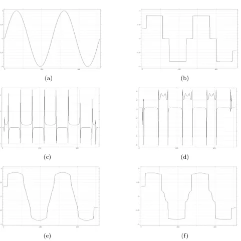
The previous result shows that the neighborhood filtering method noise is pro-portional to the second derivative of the signal. That is, it behaves like a weighted heat equation. The function f gives the sign and the magnitude of this heat equation. Where the function f takes positive values, the method noise behaves as a pure heat equation, while where it takes negative values, the method noise behaves as a reverse heat equation. The zeros and the discontinuity points of f represent the singular points where the behavior of the method changes. The magnitude of this change is much larger near the discontinuities of f producing an amplified shock effect. Figure 2.1 displays one experiment with the one dimensional neighborhood filter. We iterate the algorithm on a sine signal and illustrate the shock effect. For the two intermediate iterations un+1, we display the signal f (ρh|u′n|) which gives the sign and magnitude of
the heat equation at each point. We can see that the positions of the discontinuities of f (ρh|u′
n|) describe exactly the positions of the shocks in the further iterations and the
final state. These two examples corroborate Theorem 2.8 and show how the function f totally characterizes the performance of the one dimensional neighborhood filter.
Next we give the analogous result for 2D images. Theorem 2.9. Suppose u∈ C2(Ω), Ω
⊂ R2. Then, for 0 < ρ << h and h
→ 0 u(x)− YNFh,ρ(x)≃ − ρ2 8 (g( ρ h|Du|) uηη+ h( ρ h|Du|) uξξ), where uηη= D2u( Du |Du|, Du |Du|), uξξ = D 2u(Du⊥ |Du|, Du⊥ |Du|)
(a) (b)
(c) (d)
(e) (f)
Fig. 2.1. One dimensional neighborhood filtering experience. We iterate the filter on the sine signal until it converges to a steady state. We show the input signal (a) and the final state (b). The figures (e) and (f ) display two intermediate states. Figures (c) and (d) display the signal f (hρ|u′
n|)
which gives the magnitude and signal of the heat equation leading to figures (e) and (f ). These two signals describe exactly the positions of the shocks in the further iterations and the final state.
and g(t) = 1− 3 2t 2 1−1 4t2 , h(t) = 1− 1 2t 2 1−1 4t2 .
Proof. Let x∈ Ω and h, ρ ∈ R+. Then
u(x)−YNFh,ρ(x) =− 1 R Bρ(0)e −(u(x+th2)−u(x))2 dt Z Bρ(0)
(u(x+t)−u(x))e−(u(x+th2)−u(t))2 dt.
We take the Taylor expansion of u(x + t), and the exponential function e−y2. Then,
we take polar coordinates and integrate, obtaining
u(x)− YNFh,ρ(x)≃ 1 πρ2−ρ4π 4h2(u2x+ u2y) µ πρ4 8 ∆u− πρ6 16h2¡u 2 xuxx+ u2yuxx+ +u2xuyy+ u2xuxx¢ −πρ 6 8h2(u 2 xuxx+ 2uxuyuxy+ u2yuyy) ¶
for ρ small enough. By grouping the terms of above expression, we get the desired result.
The neighborhood filtering method noise can be written as the sum of a diffusion term in the tangent direction uξξ, plus a diffusion term in the normal direction, uηη.
The sign and the magnitude of both diffusions depend on the sign and the magnitude of the functions g and h. Both functions can take positive and negative values. There-fore, both diffusions can appear as a directional heat equation or directional reverse heat equation depending on the value of the gradient. As in the one dimensional case, the algorithm performs like a filtering / enhancing algorithm depending on the value of the gradient. If B1 =
√
2/√3 and B2 =√2 respectively denote the zeros of the functions g and h, we can distinguish the following cases:
• When 0 < |Du| < B2hρ the algorithm behaves like the Perona-Malik filter
[28]. In a first step, a heat equation is applied but when |Du| > B1hρ the
normal diffusion turns into a reverse diffusion enhancing the edges, while the tangent diffusion stays positive.
• When |Du| > B2hρ the algorithm differs from the Perona-Malik filter. A heat
equation or a reverse heat equation is applied depending on the value of the gradient. The change of behavior between these two dynamics is marked by an asymptotical discontinuity leading to an amplified shock effect.
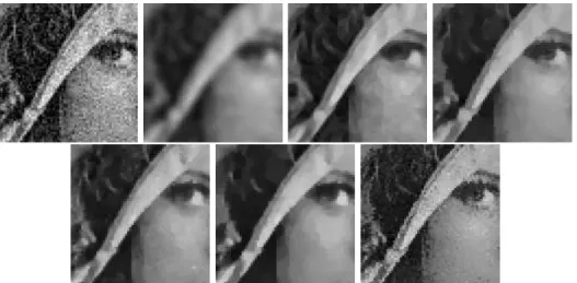
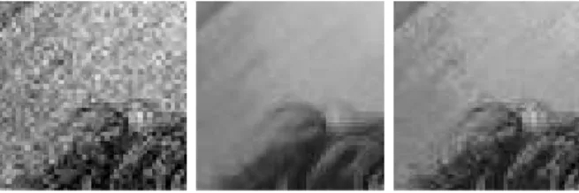
Fig. 2.2. Denoising experience on a natural image. From left to right and from top to bot-tom: noisy image (standard deviation 20), gaussian convolution, anisotropic filter, total variation minimization, Tadmor et al. iterated total variation, Osher et al. iterated total variation and the Yaroslavsky neighborhood filter.
3. Frequency domain filters. Let u be the original image defined on the grid I. The image is supposed to be modified by the addition of a signal independent white noise N . N is a random process where N (i) are i.i.d, zero mean and have constant variance σ2. The resulting noisy process depends on the random noise component,
and therefore is modelled as a random field V , V (i) = u(i) + N (i). (3.1)
Given a noise observation n(i), v(i) denotes the observed noisy image, v(i) = u(i) + n(i).
LetB = {gα}α∈Abe an orthogonal basis of R|I|. The noisy process is transformed as VB(α) = uB(α) + NB(α), (3.3) where VB(α) =hV, gαi, uB(α) =hu, gαi, NB(α) =hN, gαi
are the scalar products of V, u and N with gα ∈ B. The noise coefficients NB(α)
remain uncorrelated and zero mean, but the variances are multiplied bykgαk2,
E[NB(α)NB(β)] = X
m,n∈I
gα(m)gβ(n)E[N (m)N (n)]
=hgα, gβiσ2= σ2kgαk2δ[α− β].
Frequency domain filters are applied independently to every transform coefficient VB(α) and then the solution is estimated by the inverse transform of the new coef-ficients. Noisy coefficients VB(α) are modified to a(α)VB(α). This is a non linear algorithm because a(α) depends on the value VB(α). The inverse transform yields the estimate ˆ U = DV = X α∈A a(α) VB(α) gα. (3.4)
D is also called a diagonal operator. Let us look for the frequency domain filter D which minimizes a certain estimation error. This error is based on the square euclidean distance, and it is averaged over the noise distribution.
Definition 3.1. Let u be the original image, N a white noise and V = u + N . Let D be a frequency domain filter. Define the risk of D as
r(D, u) = E{||u − DV ||2
}, (3.5)
where the expectation is taken over the noise distribution.
The following theorem, which is easily proved, gives the diagonal operator Dinf
that minimizes the risk,
Dinf = arg min
D r(D, u).
Theorem 3.2. The operator Dinf which minimizes the risk is given by the family
{a(α)}α, where a(α) = |uB(α)| 2 |uB(α)|2+kgαk2σ2 , (3.6)
and the corresponding risk is
rinf (u) =X s∈S kgαk4 |uB (α)|2σ2 |uB(α)|2+kgαk2σ2 . (3.7)
The previous optimal operator attenuates all noisy coefficients in order to mini-mize the risk. If one restricts a(α) to be 0 or 1, one gets a projection operator. In that case, a subset of coefficients is kept and the rest gets cancelled. The projection operator that minimizes the risk r(D, u) is obtained by the following family{a(α)}α,
where a(α) = ½ 1 |uB(α)|2 ≥ ||gα||2σ2 0 otherwise and the corresponding risk is
rp(u) =X ||gα||2min(|uB(α)|2,||gα||2σ2).
Note that both filters are ideal operators because they depend on the coefficients uB(α) of the original image, which are not known. We call, as classical, Fourier Wiener Filter the optimal operator (3.6) whereB is a Fourier Basis. This is an ideal filter, since it uses the (unknown) Fourier transform of the original image. By the use of the Fourier basis (see Figure 3.1), global image characteristics may prevail over local ones and create spurious periodic patterns. To avoid this effect, the basis must take into account more local features, as the wavelet and local DCT transforms do. The search for the ideal basis associated with each image still is open. At the moment, the way seems to be a dictionary of basis instead of one single basis, [19].
Fig. 3.1. Fourier Wiener filter experiment. Top Left: Degraded image by an additive white noise of σ = 15. Top Right: Fourier Wiener filter solution. Down: Zoom on three different zones of the solution. The image is filtered as a whole and therefore a uniform texture is spread all over the image.
3.1. Local adaptive filters in transform Domain. The local adaptive filters have been introduced by L. Yaroslavsky [42, 41]. In this case, the noisy image is analyzed in a moving window and in each position of the window its spectrum is computed and modified. Finally, an inverse transform is used to estimate only the signal value in the central pixel of the window.
Let i ∈ I be a pixel and W = W (i) a window centered in i. Then the DCT transform of W is computed and modified. The original image coefficients of W, uB,W(α) are estimated and the optimal attenuation of Theorem 3.2 is applied. Finally, only the center pixel of the restored window is used. This method is called the Empirical Wiener Filter. In order to approximate uB,W(α) one can take averages on the additive noise model, that is,
E|VB,W(α)|2=
|uB,W(α)|2+ σ2||gα||2.
Denoting by µ = σ||gα||, the unknown original coefficients can be written as
|uB,W(α)|2= E|VB,W(α)|2− µ2.
The observed coefficients |vB,W(α)|2 are used to approximate E
|VB,W(α)|2, and the
estimated original coefficients are replaced in the optimal attenuation, leading to the family{a(α)}α, where
a(α) = max ½ 0,|vB,W(α)| 2− µ2 |vB,W(α)|2 ¾ .
Denote by EW Fµ(i) the filter given by the previous family of coefficients. The method
noise of the EW Fµ(i) is easily computed, as proved in the following theorem.
Theorem 3.3. Let u be an image defined in a grid I and let i ∈ I be a pixel. Let W = W (i) be a window centered in the pixel i. Then the method noise of the EWFµ(i) is given by
u(i)− EWFµ(i) =
X α∈Λ vB,W(α) gα(i) + X α /∈Λ µ2 |vB,W(α)|2 vB,W(α) gα(i). where Λ ={α | |vB,W(α)| < µ}.
The presence of an edge in the window W will produce a great amount of large coefficients and as a consequence, the cancelation of these coefficients will produce oscillations. Then, spurious cosines will also appear in the image under the form of chessboard patterns, see Figure 3.2.
3.2. Wavelet thresholding. Let B = {gα}α∈A be an orthonormal basis of
wavelets [20]. Let us discuss two procedures modifying the noisy coefficients, called wavelet thresholding methods (D. Donoho et al. [10]). The first procedure is a projec-tion operator which approximates the ideal projecprojec-tion (3.6). It is called hard thresh-olding, and cancels coefficients smaller than a certain threshold µ,
a(α) = ½
1 |vB(α)| > µ
0 otherwise
Let us denote this operator by HWTµ(v). This procedure is based on the idea that
the image is represented with large wavelet coefficients, which are kept, whereas the noise is distributed across small coefficients, which are canceled. The performance of the method depends on the capacity of approximating u by a small set of large coefficients. Wavelets are for example an adapted representation for smooth functions. Theorem 3.4. Let u be an image defined in a grid I. The method noise of a hard thresholding HWTµ(u) is
u− HWTµ(u) =
X
{α||uB(α)|<µ}
Unfortunately, edges lead to a great amount of wavelet coefficients lower than the threshold, but not zero. The cancelation of these wavelet coefficients causes small oscillations near the edges, i.e. a Gibbs-like phenomenon. Spurious wavelets can also be seen in the restored image due to the cancelation of small coefficients : see Figure 3.2. This artifact will be called: wavelet outliers, as it is introduced in [12]. D. Donoho [9] showed that these effects can be partially avoided with the use of a soft thresholding, a(α) = ( v B(α)−sgn(vB(α))µ vB(α) |vB(α)| ≥ µ 0 otherwise
which will be denoted by SWT µ(v). The continuity of the soft thresholding operator better preserves the structure of the wavelet coefficients, reducing the oscillations near discontinuities. Note that a soft thresholding attenuates all coefficients in order to reduce the noise, as an ideal operator does. As we shall see at the end of this paper, the L2norm of the method noise is lessened when replacing the hard by a soft
threshold. See Figures 3.2 and 6.3 for a comparison of the both method noises. Theorem 3.5. Let u be an image defined in a grid I. The method noise of a soft thresholding SWTµ(u) is u− SWTµ(u) = X {α||uB(α)|<µ} uB(α)gα+ µ X {α||uB(α)|>µ} sgn(uB(α)) gα
A simple example can show how to fix the threshold µ. Suppose the original image u is zero, then vB(α) = nB(α), and therefore the threshold µ must be taken over the maximum of noise coefficients to ensure their suppression and the recovery of the original image. It can be shown that the maximum amplitude of a white noise has a high probability of being smaller than σp2 log |I|. It can be proved that the risk of a wavelet thresholding with the threshold µ = σp2 log |I| is near the risk rp
of the optimal projection, see [10, 20].
Theorem 3.6. The risk rt(u) of a hard or soft thresholding with the threshold
µ = σp2 log |I| is such that for all |I| ≥ 4
rt(u)≤ (2 log |I| + 1)(σ2+ rp(u)).
(3.8)
The factor 2 log|I| is optimal among all the diagonal operators in B, that is,
lim |I|−>∞D∈DinfB sup u∈R|I| E{||u − DV ||2 } σ2+ r p(u) 1 2log|I| = 1. (3.9)
In practice the optimal threshold µ is very high and cancels too many coefficients not produced by the noise. A threshold lower than the optimal is used in the experi-ments and produces much better results, see Figure 3.2. For a hard thresholding the threshold is fixed to 3∗ σ. For a soft thresholding this threshold still is too high ; it is better fixed at 3
2σ.
3.3. Translation invariant wavelet thresholding. R. Coifman and D. Donoho [8] improved the wavelet thresholding methods by averaging the estimation of all trans-lations of the degraded signal. Calling vp(i) the translated signal v(i− p), the wavelet
coefficients of the original and translated signals can be very different, and they are not related by a simple translation or permutation,
vpB(α) =hv(n − p), gα(n)i = hv(n), gα(n + p)i.
The vectors gα(n + p) are not in general in the basisB = {gα}α∈A, and therefore the
estimation of the translated signal is not related to the estimation of v. This new algorithm yields an estimate ˆup for every translated vp of the original image,
ˆ
up= Dvp=X
α∈A
a(α)vBp(α)gα.
(3.10)
The translation invariant thresholding is obtained by averaging all these estimators after a translation in the inverse sense,
1 |I| X p∈I ˆ up(i + p), (3.11)
and will be denoted by TIWT (v).
The Gibbs effect is considerably reduced by the translation invariant wavelet thresholding, (see Figure 3.2), because the average of different estimations of the image reduces the oscillations. This is therefore the version we shall use in the comparison section. Recently, S. Durand and M. Nikolova [12] have actually proposed an efficient variational method finding the best compromise to avoid the three common artifacts in TV methods and wavelet thresholding, namely the stair-casing, the Gibbs effect and the wavelet outliers. Unfortunately, we couldn’t draw the method into the comparison.
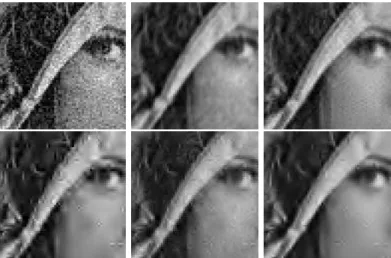
Fig. 3.2. Denoising experiment on a natural image. From left to right and from top to bottom: noisy image (standard deviation 20), Fourier Wiener filter (ideal filter), the DCT empirical Wiener filter, the wavelet hard thresholding, the soft wavelet thresholding and the translation invariant wavelet hard thresholding.
4. Statistical neighborhood approaches. The methods we are going to con-sider are very recent attempts to take advantage of an image model learned from the image itself. More specifically, these denoising methods attempt to learn the statisti-cal relationship between the image values in a window around a pixel and the pixel value at the window center.
4.1. DUDE, a universal denoiser. The recent work by Ordentlich et al. [39] has led to the proposition of a “universal denoiser” for digital images. The authors assume that the noise model is fully known, namely the probability transition matrix Π(a, b) , where a, b ∈ A, the finite alphabet of all possible values for the image. In order to fix ideas, we shall assume as in the rest of this paper that the noise is additive gaussian, in which case one simply has Π(a, b) = √1
2πσe
−(a−b)22σ2 for the probability of
observing b when the real value was a. The authors also fix an error cost Λ(a, b) which, to fix ideas, we can take to be a quadratic function Λ(a, b) = (a− b)2, namely
the cost of mistaking a for b.
The authors fix a neighborhood shape, say, a square discrete window deprived of its center i, ˜Ni= Ni\ {i} around each pixel i. Then the question is : once the image
has been observed in the window ˜Ni, what is the best estimate we can make from the
observation of the full image ?
The authors propose the following algorithm:
• Compute, for each possible value b of u(i) the number of windows Nj in
the image such the restrictions of u to ˜Nj and ˜Ni coincide and the observed
value at the pixel j is b. This number is called m(b, Ni) and the line vector
(m(b, Ni))b∈A is denoted by m(Ni).
• Then, compute the denoised value of u at i as ˜
u(i) = arg min
b∈Am(Ni)Π −1(Λ
b⊗ Πu(i)),
where w⊗ v = (w(b)v(b)) denotes the vector obtained by multiplying each component of u by each component of v, u(i) is the observed value at i, and we denote by Xa the a-column of a matrix X.
The authors prove that this denoiser is universal in the sense “of asymptotically achieving, without access to any information on the statistics of the clean signal, the same performance as the best denoiser that does have access to this information”. In [24] the authors present an implementation valid for binary images with an impulse noise, with excellent results. The reason of these limitations in implementation are clear : first the matrix Π is of very low dimension and invertible for impulse noise. If instead we consider as above a gaussian noise, then the application of Π−1 amounts
to deconvolve a signal by a gaussian, which is a rather ill-conditioned method. All the same, it is doable, while the computation of m certainly is not for a large alphabet, like the one involved in grey tone images (256 values). Even supposing that the learning window Nihas the minimal possible size of 9, the number of possible such windows is
about 2569which turns out to be much larger than the number of observable windows
in an image (whose typical size amounts to 106 pixels). Actually, the number of
samples can be made significantly smaller by quantizing the grey level image and by noting that the window samples are clustered. Anyway, the direct observation of the number m(Ni) in an image is almost hopeless, particularly if it is corrupted by noise.
4.2. The UINTA algorithm. Awate and Whitaker [3] have proposed a method whose principles stand close to the the NL-means algorithm, since, as in Dude, the method involves comparison between subwindows to estimate a restored value. The objective of the algorithm ”UINTA, for unsupervised information theoretic adaptive filter”, is to denoise the image decreasing the randomness of the image. The algorithm proceeds as follows:
• Assume that the (2d + 1) × (2d + 1) windows in the image are realizations of a random vector Z. The probability distribution function of Z is estimated
from the samples in the image, p(z) = 1 |A| X zi∈A Gσ(z− zi), where z ∈ R(2d+1)×(2d+1), G
σ is the gaussian density function in dimension
n with variance σ2,
Gσ(x) = 1
(2π)n2σe
−||xσ2||2,
and A is a random subset of windows in the image.
• Then the authors propose an iterative method which minimizes the entropy of the density distribution,
Eplog p(Z) =−
Z
p(z) log p(z)dz.
This minimization is achieved by a gradient descent algorithm of the previous energy function.
The denoising effect of this algorithm can be understood, as it forces the proba-bility density to concentrate. Thus, groups of similar windows tend to assume a more and more similar configuration which is less noisy. The differences of this algorithm with NL-means are patent, however. This algorithm creates a global interaction be-tween all windows. In particular, it tends to favor big groups of similar windows and to remove small groups. In that extent, it is a global homogenization process and is quite valid if the image consists of a periodic or quasi periodic texture, as is patent in the successful experiments shown in this paper. The spirit of this method is to define a new, information theoretically oriented scale space. In that sense, the gradi-ent descgradi-ent must be stopped before a steady state. The time at which the process is stopped gives us the scale of randomness of the filtered image.
5. Non local means algorithm (NL-means). The local smoothing methods and the frequency domain filters aim at a noise reduction and at a reconstruction of the main geometrical configurations but not at the preservation of the fine structure, details and texture. Due to the regularity assumptions on the original image of pre-vious methods, details and fine structures are smoothed out because they behave in all functional aspects as noise. The NL-means algorithm we shall now discuss tries to take advantage of the high degree of redundancy of any natural image. By this, we simply mean that every small window in a natural image has many similar windows in the same image. This fact is patent for windows close by, at one pixel distance and in that case we go back to a local regularity assumption. Now in a very general sense inspired by the neighborhood filters, one can define as “neighborhood of a pixel i” any set of pixels j in the image such that a window around j looks like a window around i. All pixels in that neighborhood can be used for predicting the value at i, as was first shown in [13] for 2D images. This first work has inspired many variants for the restoration of various digital objects, in particular 3D surfaces [33]. The fact that such a self-similarity exists is a regularity assumption, actually more general and more accurate than all regularity assumptions we have considered in section 2. It also generalizes a periodicity assumption of the image.
Let v be the noisy image observation defined on a bounded domain Ω⊂ R2and
values of all the pixels whose gaussian neighborhood looks like the neighborhood of x, N L(v)(x) = 1 C(x) Z Ω e−(Ga∗|v(x +.)−v(y+.)|2 )(0) h2 v(y) dy,
where Ga is a Gaussian kernel with standard deviation a, h acts as a filtering
pa-rameter and C(x) =R
Ωe−
(Ga∗|v(x+.)−v(z+.)|2 )(0)
h2 dz is the normalizing factor. We recall
that,
(Ga∗ |v(x + .) − v(y + .)|2)(0) =
Z
R2
Ga(t)|v(x + t) − v(y + t)|2dt.
Since we are considering images defined on a discrete grid I, we shall give a discrete description of the NL-means algorithm and some consistency results. This simple and generic algorithm and its application to the improvement of the performance of digital cameras is the object of an European patent application [4].
5.1. Description. Given a discrete noisy image v ={v(i) | i ∈ I}, the estimated value N L(v)(i) is computed as a weighted average of all the pixels in the image,
N L(v)(i) =X
j∈I
w(i, j)v(j),
where the weights{w(i, j)}j depend on the similarity between the pixels i and j, and
satisfy the usual conditions 0≤ w(i, j) ≤ 1 andP
jw(i, j) = 1.
In order to compute the similarity between the image pixels, we define a neigh-borhood system on I.
Definition 5.1 (Neighborhoods). A neighborhood system on I is a family N = {Ni}i∈I of subsets of I such that for all i∈ I,
(i) i∈ Ni,
(ii) j∈ Ni⇒ i ∈ Nj.
The subsetNi is called the neighborhood or the similarity window of i. We set ˜Ni =
Ni\{i}.
The similarity windows can have different sizes and shapes to better adapt to the image. For simplicity we will use square windows of fixed size. The restriction of v to a neighborhoodNi will be denoted by v(Ni),
v(Ni) = (v(j), j∈ Ni).
The similarity between two pixels i and j will depend on the similarity of the intensity gray level vectors v(Ni) and v(Nj). The pixels with a similar grey level
neighborhood to v(Ni) will have larger weights in the average, see Figure 5.1.
In order to compute the similarity of the intensity gray level vectors v(Ni) and
v(Nj), one can compute a gaussian weighted Euclidean distance,kv(Ni)− v(Nj)k22,a.
Efros and Leung [13] showed that the L2 distance is a reliable measure for the
com-parison of image windows in a texture patch. Now, this measure is so much the more adapted to any additive white noise as such a noise alters the distance between windows in a uniform way. Indeed,
Fig. 5.1. q1 and q2 have a large weight because their similarity windows are similar to that of p. On the other side the weight w(p,q3) is much smaller because the intensity grey values in the similarity windows are very different.
where u and v are respectively the original and noisy images and σ2 is the noise
variance. This equality shows that, in expectation, the Euclidean distance preserves the order of similarity between pixels. So the most similar pixels to i in v also are expected to be the most similar pixels to i in u. The weights associated with the quadratic distances are defined by
w(i, j) = 1 Z(i)e −||v(Ni)−v(Nj )|| 2 2,a h2 ,
where Z(i) is the normalizing factor Z(i) =P
je−
||v(Ni)−v(Nj )||2 2,a
h2 and the parameter
h controls the decay of the exponential function and therefore the decay of the weights as a function of the Euclidean distances.
5.2. A consistency theorem for NL-means. The NL-means algorithm is intuitively consistent under stationarity conditions, saying that one can find many samples of every image detail. In fact, we shall be assuming that the image is a fairly general stationary random process. Under these assumptions, for every pixel i, the NL-means algorithm converges to the conditional expectation of i knowing its neighborhood. In the case of an additive or multiplicative white noise model, this expectation is in fact the solution to a minimization problem.
Let X and Y denote two random vectors with values on Rpand R respectively. Let
fX, fY denote the probability distribution functions of X, Y and let fXY denote the
joint probability distribution function of X and Y . Let us recall briefly the definition of the conditional expectation.
Definition 5.2.
i) Define the probability distribution function of Y conditioned to X as
f (y| x) = ( f
XY(x,y)
fX(x) if fX(x) > 0
0 otherwise for all x∈ Rp and y∈ R.
ii) Define the conditional expectation of Y given {X = x} as the expectation with respect to the conditional distribution f (y| x)
E[Y | X = x] = Z
for all x∈ Rp.
The conditional expectation is a function of X and therefore a new random vari-able g(X) which is denoted by E[Y | X].
Let now V be a random field andN a neighborhood system on I. Let Z denote the sequence of random variables Zi={Yi, Xi}i∈Iwhere Yi= V (i) is real valued and
Xi = V ( ˜Ni) is Rp valued. Recall that ˜Ni=Ni\{i}.
Let us restrict Z to the n first elements {Yi, Xi}ni=1. Let us define the function
rn(x), rn(x) = Rn(x)/ ˆfn(x) (5.1) where ˆ fn(x) = 1 nhp n X i=1 K(Xi− x h ), Rn(x) = 1 nhp n X i=1 φ(Yi)K( Xi− x h ), (5.2)
φ is an integrable real valued function, K is a nonnegative kernel and x∈ Rp.
Let X and Y be distributed as X1 and Y1. Under this form the NL-means
algorithm can be seen as an instance for the exponential operator of the Nadaraya-Watson estimator [23, 38]. This is an estimator of the conditional expectation r(x) = E[φ(Y )| X = x]. Some definitions are needed for the statement of the main result.
Definition 5.3. A stochastic process {Zt | t = 1, 2, . . .}, with Zt defined on
some probability space (Ω,A, P), is said to be (strict-sense) stationary if for any finite partition{t1, t2,· · · , tn} the joint distributions Ft1,t2,···,tn(x1, x2,· · · , xn) are the same
as the joint distributions Ft1+τ,t2+τ,···,tn+τ(x1, x2,· · · , xn) for any τ ∈ N .
In the case of images, this stationary condition amounts to say that as the size of the image grows, we are able to find in the image many similar patches for all the details of the image. This is a crucial point to understand the performance of the NL-means algorithm. The following mixing definition is a rather technical condition. In the case of images, it amounts to say that regions become more independent as their distance increases. This is intuitively true for natural images.
Definition 5.4. Let Z be a stochastic and stationary process{Zt| t = 1, 2, · · · , n},
and, for m < n, let Fn
m be the σ− field induced in Ω by the r.v.’s Zj, m≤ j ≤ n.
Then, the sequence Z is said to be β−mixing if for every A ∈ Fk
1 and every B∈ F∞k+n
|P (A ∩ B) − P (A)P (B)| ≤ β(n) with β(n) → 0, as n → ∞.
The following theorem establishes the convergence of rn to r, see Roussas [29].
The theorem is established under the stationary and mixing hypothesis of{Yi, Xi}∞i=1
and asymptotic conditions on the decay of φ, β(n) and K. This set of conditions will be denoted by H and it is more carefully detailed in the Appendix.
Theorem 5.5 (Conditional expectation theorem). Let Zj ={Xj, Yj} for j =
1, 2,· · · be a strictly stationary and mixing process. For i ∈ I, let X and Y be dis-tributed as Xi and Yi. Let J be a compact subset J ⊂ Rp such that
inf{fX(x); x∈ J} > 0.
Then, under hypothesis H,
where ψn are positive norming factors.
Let v be the observed noisy image and let i be a pixel. Taking for φ the identity, we see that rn(v( ˜Ni)) converges to E[V (i) | V ( ˜Ni) = v( ˜Ni)] under stationary and
mixing conditions of the sequence{V (i), V ( ˜Ni)}∞i=1.
In the case where an additive or multiplicative white noise model is assumed, the next result shows that this conditional expectation is in fact the function of V ( ˜Ni)
that minimizes the mean square error with the original field U .
Theorem 5.6. Let V, U, N1, N2 be random fields on I such that V = U + N1+
g(U )N2, where N1 and N2 are independent white noises. Let N be a neighborhood
system on I . Then,
(i) E[V (i)| V ( ˜Ni) = x] = E[U (i)| V ( ˜Ni) = x] for all i∈ I and x ∈ Rp.
(ii) The real value E[U (i) | V ( ˜Ni) = x] minimizes the following mean square
error, min g∗∈RE[(U (i)− g ∗)2 | V ( ˜Ni) = x] (5.3)
for all i∈ I and x ∈ Rp.
(iii) The expected random variable E[U (i)| V ( ˜Ni)] is the function of V ( ˜Ni) that
minimizes the mean square error min
g E[U (i)− g(V ( ˜Ni))] 2
(5.4)
Given a noisy image observation v(i) = u(i) + n1(i) + g(u(i))n2(i), i∈ I, where
g is a real function and n1 and n2 are white noise realizations, then the NL-means
algorithm is the function of v( ˜Ni) that minimizes the mean square error with the
original image u(i).
5.3. Experiments with NL-means. The NL-means algorithm chooses for each pixel a different average configuration adapted to the image. As we explained in the previous sections, for a given pixel i, we take into account the similarity between the neighborhood configuration of i and all the pixels of the image. The similarity between pixels is measured as a decreasing function of the Euclidean distance of the similarity windows. Due to the fast decay of the exponential kernel, large Euclidean distances lead to nearly zero weights, acting as an automatic threshold. The decay of the exponential function and therefore the decay of the weights is controlled by the parameter h. Empirical experimentation shows that one can take a similarity window of size 7× 7 or 9 × 9 for grey level images and 5 × 5 or even 3 × 3 in color images with little noise. These window sizes have shown to be large enough to be robust to noise and at the same time to be able to take care of the details and fine structure. Smaller windows are not robust enough to noise. Notice that in the limit case, one can take the window reduced to a single pixel i and get therefore back to the Yaroslavsky neighborhood filter. We have seen experimentally that the filtering parameter h can take values between 10∗ σ and 15 ∗ σ, obtaining a high visual quality solution. In all experiments this parameter has been fixed to 12∗σ. For computational aspects, in the following experiments the average is not performed in all the image. In practice, for each pixel p, we only consider a squared window centered in p and size 21× 21 pixels. The computational cost of the algorithm and a fast multiscale version is addressed in section 5.5.
Due to the nature of the algorithm, the most favorable case for the NL-means is the periodic case. In this situation, for every pixel i of the image one can find a large
Fig. 5.2. NL-means denoising experiment with a nearly periodic image. Left: Noisy image with standard deviation 30. Right: NL-means restored image.
set of samples with a very similar configuration, leading to a noise reduction and a preservation of the original image, see Figure 5.2 for an example.
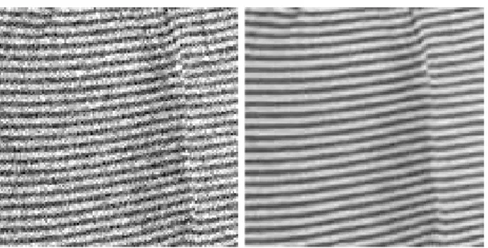
Fig. 5.3. NL-means denoising experiment with a Brodatz texture image. Left: Noisy image with standard deviation 30. Right: NL-means restored image. The Fourier transform of the noisy and restored images show how main features are preserved even at high frequencies.
Another case which is ideally suitable for the application of the NL-means al-gorithm is the textural case. Texture images have a large redundancy. For a fixed configuration many similar samples can be found in the image. In Figure 5.3 one can see an example with a Brodatz texture. The Fourier transform of the noisy and restored images shows the ability of the algorithm to preserve the main features even in the case of high frequencies.
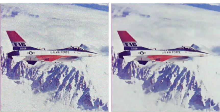
NL-means is not only able to restore periodic or texture images. Natural images also have enough redundancy to be restored. For example in a flat zone, one can find many pixels lying in the same region and similar configurations. In a straight or curved edge a complete line of pixels with a similar configuration is found. In addition, the redundancy of natural images allows us to find many similar configurations in far away pixels. Figures 5.4 and 5.5 show two examples on two well known standard processing images. The same algorithm applies to the restoration of color images and films, see Figure 5.6.
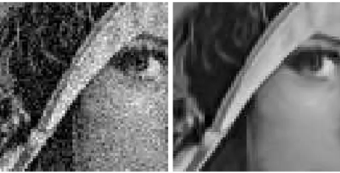
Fig. 5.4. NL-means denoising experiment with a natural image. Left: Noisy image with stan-dard deviation 20. Right: Restored image.
Fig. 5.5. NL-means denoising experiment with a natural image. Left: Noisy image with stan-dard deviation 35. Right: Restored image.
5.4. Testing stationarity : a soft threshold optimal correction. In this section, we describe a simple and useful statistical improvement of NL-means, with a technique similar to the wavelet thresholding. The stationarity assumption of Theo-rem 5.5 is not true everywhere, as each image may contain exceptional, non repeated structures. Such structures can be blurred out by the algorithm. The NL-means al-gorithm, and actually every local averaging alal-gorithm, must involve a detection phase and special treatment of non stationary points. The principle of such a correction is quite simple and directly derived from other thresholding methods, like the SWT method.
Let us estimate the original value at a pixel i, u(i), as the mean of the noisy grey levels v(j) for j∈ J ⊂ I. In order to reduce the noise and restore the original value, pixels j ∈ J should have a non noisy grey level u(j) similar to u(i). Assuming this fact, ˆ u(i) = 1 |J| X j∈J v(j)≃ 1 |J| X j∈J u(i) + n(j)→ u(i) as |J| → ∞,
because the average of noise values tends to zero. In addition, 1 |J| X j∈J (v(j)− ˆu(i))2≃ 1 |J| X j∈J n(j)2→ σ2 as|J| → ∞.
If the averaged pixels have a non noisy grey level value close to u(i), as expected, then the variance of the average should be close to σ2. If it is a posteriori observed that