Supporting Information (SI) for
“Toward link predictability of complex networks”
by Linyuan L¨
u, Liming Pan, Tao Zhou, Yi-Cheng Zhang, and H. Eugene Stanley
I. CASE OF DEGENERATE EIGENVALUES
If the adjacency matrix contains degenerate eigenvalues, we must modify the approach using non-degenerate eigen-values. We denote the eigenvalues as λki, where the index k runs over different eigenvalues and the index i runs over M associated eigenvectors of the same eigenvalue. Note that there is no unique way of choosing a basis for the eigenvectors of the unperturbed network since any linear combination of the eigenvectors belonging to the same eigen-value is still an eigenvector. Repeated eigeneigen-values have been shown to be related to the symmetric motifs and graph automorphisms in networks [1]. After a perturbation is added to the network, the symmetry of the nodes will be lifted either partly or completely, so the degenerate eigenvalues must be chosen such that they can be transformed contin-uously into the perturbed non-degenerate eigenvalues. If we define the chosen eigenvectors to be ¯xki=∑Mj=1βkjxkj, the eigenfunction becomes
( AR+ ∆A)x¯ki= ( λki+ ∆¯λki ) ¯ xki, (1) giving us ∆¯λki M ∑ j=1 βkjxkj= M ∑ j=1 βkj∆Axkj. (2)
For any n = 1· · · M, left multiplying Eq. (2) by xT
kn, we obtain ∆¯λkiβkn= M ∑ j=1 βkjxTkn∆Axkj. (3)
Written in matrix form, Eq. (3) becomes
W Bk= ∆¯λkBk, (4)
where W is an M × M matrix and is defined by Wnj = xT
kn∆Axkj and Bk is the column vector of βkj. After obtaining ∆¯λk and Bk from the eigenfunction (4), the corrected eigenvectors as well as the first-order corrections to the corresponding eigenvalues can be determined simultaneously. Then the structural consistency can be calculated in the same way as in the non-degenerate eigenvalues case. Specifically, to obtain the perturbed adjacency matrix ˜A we simply replace xk and ∆λk in Eq. 4 with ¯xk and ∆¯λk, respectively.
II. SIX STEPS TO CALCULATE σc
Given a network G, we calculate the structural consistency σc via the following procedure:
Step 1: Given network A, we randomly select a fraction of links to constitute a perturbation set ∆E(∆A), while the rest is ER(AR), obviously A = AR+ ∆A .
Step 2: We calculate the eigenvalues λk and their corresponding eigenvectors (xk) of AR. Step 3: We use equation (3) to calculate ∆λ.
Step 4: We use equation (4) to calculate the perturbed matrix ˜A.
Step 5: We rank the non-observed links according to their scores given by ˜A. For a non-observed link (i, j), its score is the value of ˜Aij.
Step 6: We select the top-L non-observed links. Here L is the number of links in set ∆E. And we see how many of them are also in the perturbation set ∆E. This ratio is σc.
For example, a true network with 20 nodes has 100 links, and we select 10 links as ∆E, then there are 20×19/2−90 = 100 non-observed links. By using our method, we find among these 10 links in ∆E, there are 6 links that are ranked within the top-10 places according to their scores in ˜A. Then σc = 6/10 = 0.6.
III. LINK PREDICTION PROBLEM
The purpose of link prediction (LP) is to estimate the existence likelihood of all non-observable links based on known network topology and node attributes (assuming this information is available). We consider an undirected network G(V, E) in which V is the set of nodes and E is the set of links. Multiple links and self connections are not allowed. Denote by U the universal set containing all|V |(|V | − 1)/2 possible links, where |V | denotes the number of elements in set V . Then, the set of non-existent links is U − E. We assume that missing links exist (or will exist in the future) in the set U− E, and the task of link prediction is to locate them.
Because we do not know which links in a system are missing or will appear in the future, we test the algorithm’s accuracy by randomly dividing the observed links E (in the original network) into two sets, (i) a training set ET made up of known information, and (ii) a probe set EP used for testing and from which no information is allowed for use in prediction. Clearly, ET∪EP = E and ET∩EP =∅. In principle, a link prediction algorithm provides an ordered list of all non-observed links (i.e., U− ET) or equivalently gives each non-observed link, say (x, y)∈ U − ET, a score sxy to quantify its existence likelihood. Two standard metrics are used to quantify the accuracy of prediction algorithms: the area under the receiver operating characteristic curve (AUC) [2] and the precision [3]. The AUC evaluates the algorithm’s performance according to the entire list and the precision focuses only on the L links with the top ranks or the highest scores. The following is a detailed description of these two metrics.
(i) AUC.— Given the ranking of the non-observed links, the AUC value is the probability that a randomly chosen missing link (i.e., a link in EP) has a higher score than a randomly chosen nonexistent link (i.e., a link in U− E). In the algorithmic implementation, we usually calculate the score of each non-observed link instead of the ordered list since the latter task is more time-consuming. The computational complexity for an ordered list of nonexistent links in a sparse network isO(|V |2log|V |2). Since the number of nodes|V | can be very large, it is very time-consuming to
obtain the exact value of AUC which requires|EP|·[V (V −1)/2−|E|] pairs of comparison. Instead of the exact value, to estimate the AUC value with very good accuracy does not need to know the ordered list. At each time step we randomly pick a missing link and a nonexistent link and compare their scores. If among n independent comparisons there are n′ times the missing link that have a higher score and n′′times that have the same score, the AUC value is
AUC = n
′+ 0.5n′′
n . (5)
If all the scores are generated from an independent and identical distribution, the AUC value will be approximately 0.5. Thus the degree to which the value exceeds 0.5 indicates how much better the algorithm performs than pure chance.
(ii) Precision.— Given the ranking of the non-observed links, the precision is defined as the ratio of relevant items selected to the number of items selected. That is to say, if we take the top-L links as the predicted ones, among which Lrlinks are right (i.e., there are Lrlinks in the probe set EP), then the precision equals Lr/L. Thus a higher precision value means a higher prediction accuracy.
Figure S1 shows an example of how to calculate the AUC and the precision. In this simple network there are five nodes, seven existent links, and three nonexistent links ((1, 2), (1, 4) and (3, 4)). To test the algorithm’s accuracy, we select several existent links as probe links. For example, we can pick (1, 3) and (4, 5) as probe links (dashed lines in the right plot). Then algorithms can only use the information contained in the training network (presented by solid lines in the right plot). If an algorithm assigns scores of all non-observed links as s12 = 0.4, s13 = 0.5, s14 = 0.6,
s34= 0.5 and s45= 0.6. To calculate the AUC, we compare the scores of a probe link and a nonexistent link. There
are in total six pairs: s13> s12, s13< s14, s13= s34, s45> s12, s45= s14and s45> s34. Thus the AUC value equals
(3× 1 + 2 × 0.5)/6 ≈ 0.67. For the precision, if L = 2, the predicted links are (1, 4) and (4, 5). Clearly the former is wrong and the latter is right, and thus the precision equals 0.5.
In this paper we make predictions based solely on the known topology of the network (i.e., the information contained in training set). In real applications, generally the reliability of prediction is not revealed by the LP algorithm itself, and predictions are sometimes even quite distinct for different algorithms. σc gives a basic understanding of how predictable a network is. Intuitively speaking, σc is a metric of how the observed links and missing links are linearly consist.
IV. CORRELATION BETWEEN INDEPENDENT PERTURBATIONS
The correlation between the first-order corrections and the eigenvalues between independent perturbations is the foundation of the SPM. For the first-order perturbation, each edge acts independently of the correction of the
eigen-1 3 2 4 5 1 3 2 4 5
Original network Training network FIG. S1. An illustration about the calculation of AUC and Precision.
values. That is to say, two independent sets of the hidden edges ∆A1 and ∆A2change the eigenvalues as
∆λk= xT k∆Axk xT kxk = x T k(∆A1+ ∆A2) xk xT kxk =x T k∆A1xk xT kxk +x T k∆A2xk xT kxk = ∆λk1+ ∆λk2. (6)
The two sets are independent because they have no edges in common. We calculate the average Pearson correlation coefficient of ∆λ between independent perturbations, as shown in Table S1. ∆λ for independent perturbations are strongly correlated, implying that missing links can be predicted by perturbing the observed network. Generally, the larger the correlation r is, the higher precision SPM gives (see Table 1).
TABLE S1. Pearson correlation coefficient of ∆λ between independent perturbations. For a given network, we firstly remove two independent sets of edges, named ∆A1 and ∆A2, from the network. Then we perturb the rest network by ∆A1and ∆A2,
respectively, to obtain two group of the corrected eigenvalues.
Nets Jazz Metabolic Neural USAir Food web Hamster NetSci Yeast Email Router
r 0.920 0.778 0.758 0.837 0.882 0.853 0.592 0.680 0.663 0.781
V. FIVE STEPS TO CALCULATE PREDICTION ACCURACY OF SPM For a given network to calculate the link prediction accuracy of SPM method, we have five steps:
Step 1: We first divide the true network A into training set ET and probe set EP, obviously, A = AT+ AP. Step 2: We further divide ET into ER and ∆E.
Step 3: We use ∆E to perturb ER, and calculate ˜A following the procedures (i.e., step 2-4) for calculating σ c. Step 4: Repeat step 2 and 3 for ten times, namely we independently divide ET into ER and ∆E for ten times, then we obtain ten ˜A matrixes. Averaging the scores of ten ˜A, we obtain the final score matrix ⟨ ˜A⟩ where ⟨ ˜A⟩ij is the score of link (i, j).
Step 5: Ranking all the non-observed links (i.e., links in U− ET) in decreasing order according to their scores given by⟨ ˜A⟩, we select |EP| links on the top places and see how many of them are in the probe set. This ratio is precision.
Repeat step 1-5 n times, we obtain an average precision. In this paper, we set n = 100.
VI. STATISTICAL FEATURES OF EXPERIMENTAL NETWORKS
We consider networks from disparate areas, including social, biological, and technological networks. The networks used in the experiment are described as follows and the basic statistical features are shown in Table S2. Directed links are treated as undirected, multiple links are treated as a single unweighted link and self loops are removed. Note that for the very large networks we consider the sampled subnetworks. The detailed sampling method is introduced in section VIII, which provides us with a useful tool for addressing large-scale networks.
(i) Jazz [4]: A collaboration network of jazz musicians consists of 198 nodes and 2742 interactions. (ii) Metabolic [5]: A metabolic network of C.elegans.
(iii) Neural [6]: The neural network of C.elegans. The original network is directed and weighted; here we treat it as simple graph by simply ignore the directions and weights.
(iv) USAir [7]: The US Air transportation system.
(v) Food web [8]: A food web in Florida Bay during the rainy season.
(vi) Hamster [9]: A friendship network of users of the website hamsterster.com.
(vii) NetSci [10]: A coauthorship network of scientists working on network theory and experiment. (viii) Yeast [11]: A protein-protein interaction network in budding yeast.
(ix) Email [12]: A network of e-mail interchanges between members of the University Rovira i Virgili (Tarragona). (x) Router [13]: A symmetrized snapshot of the structure of the Internet at the level of autonomous systems. (xi) Arxiv [14]: A collaboration graph of authors of scientific papers from the arXiv’s High Energy Physics C Theory (hep-th) section. An edge between two authors represents a common publication. Timestamps denote the date of a publication.
(xii) Facebook [15]: A directed network of a small subset of posts to other user’s wall on Facebook. The nodes of the network are Facebook users, and each directed edge represents one post, linking the users writing a post to the users whose wall the post is written on. Since users may write multiple posts on a wall, the network allows multiple edges connecting a single node pair. Since users may write on their own wall, the network contains loops.
(xiii) Enron [16]: This network consists of 1,148,072 emails sent between employees of Enron between 1999 and 2003. Nodes in the network are individual employees and edges are individual emails. It is possible to send an email to oneself, and thus the original network contains loops.
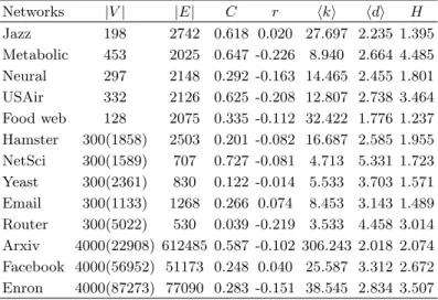
TABLE S2. The basic topological features of thirteen real networks. |V | and |E| are the number of nodes and links. C is the clustering coefficient [6] and r the assortative coefficient [17]. ⟨k⟩ is the average degree, ⟨d⟩ is the average shortest distance, and H is the degree heterogeneity, as H =⟨k2⟩/⟨k⟩2
. Note that for the sampled subnetwork,|V | of the original network are shown in the bracket.
Networks |V | |E| C r ⟨k⟩ ⟨d⟩ H Jazz 198 2742 0.618 0.020 27.697 2.235 1.395 Metabolic 453 2025 0.647 -0.226 8.940 2.664 4.485 Neural 297 2148 0.292 -0.163 14.465 2.455 1.801 USAir 332 2126 0.625 -0.208 12.807 2.738 3.464 Food web 128 2075 0.335 -0.112 32.422 1.776 1.237 Hamster 300(1858) 2503 0.201 -0.082 16.687 2.585 1.955 NetSci 300(1589) 707 0.727 -0.081 4.713 5.331 1.723 Yeast 300(2361) 830 0.122 -0.014 5.533 3.703 1.571 Email 300(1133) 1268 0.266 0.074 8.453 3.143 1.489 Router 300(5022) 530 0.039 -0.219 3.533 4.458 3.014 Arxiv 4000(22908) 612485 0.587 -0.102 306.243 2.018 2.074 Facebook 4000(56952) 51173 0.248 0.040 25.587 3.312 2.672 Enron 4000(87273) 77090 0.283 -0.151 38.545 2.834 3.507
VII. LINK PREDICTION ON REAL NETWORKS
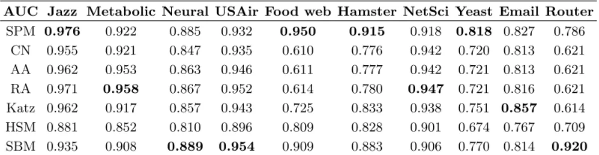
We compare our method, structural perturbation method (SPM), to several well-known methods, including three local algorithms based on the number of common neighbors between pairs of nodes (CN, AA and RA), a path-dependent global method (Katz), and the approaches of Clauset et al. (HSM) and Guimer`a et al. (SBM). For the definition of each algorithm see the Materials and Methods. For each real network a fraction of its links Ep will be removed to constitute the probe set which, in our experiments, always contain 10% of links in E. The rest of the links constitute the training set ET used to generate an observable network. Using the LP methods we then calculate the existence likelihood of each node pair not connected in the observed network, and rank the node pairs in order of decreasing existence likelihood. Prediction accuracy is obtained by precision and AUC respectively, see the definition of these two evaluation metrics in Materials and Methods. We set pH= 0.1 for SPM and L =|0.1E| to calculate the precision. For the parameter-dependent Katz index, the present results are obtained under the optimal parameter α subject to the highest precision.
TABLE S3. Link prediction accuracy measured by AUC on the ten real networks.
AUC Jazz Metabolic Neural USAir Food web Hamster NetSci Yeast Email Router
SPM 0.976 0.922 0.885 0.932 0.950 0.915 0.918 0.818 0.827 0.786 CN 0.955 0.921 0.847 0.935 0.610 0.776 0.942 0.720 0.813 0.621 AA 0.962 0.953 0.863 0.946 0.611 0.777 0.942 0.721 0.813 0.621 RA 0.971 0.958 0.867 0.952 0.614 0.780 0.947 0.721 0.816 0.621 Katz 0.962 0.917 0.857 0.943 0.725 0.833 0.938 0.751 0.857 0.614 HSM 0.881 0.852 0.810 0.896 0.809 0.828 0.901 0.674 0.767 0.709 SBM 0.935 0.908 0.889 0.954 0.909 0.883 0.906 0.770 0.814 0.920
VIII. APPLYING TO LARGE NETWORKS
To apply our method to large networks, we use random walk sampling [18] to obtain a subnetwork. We do this by randomly picking a starting node and then using the random walk to select the subnetwork. At each time step there is a probability c = 0.15 that the random walk will jump back to the staring node. This procedure is continued until the desired number of nodes are selected. When the network is extremely large and computing the full spectrum unpractical, we calculate the σc of the sampled subnetwork to determine its link predictability. Figure S2 shows how the subnetwork sampled using the random walk method can successfully recover the σc of the original network. This enables us to approximate the predictability of large networks using the sampled subnetwork.
0.0 0.2 0.4 0.6 0.8 1.0 0.1 0.2 0.3 0.4 0.5 0.6 0.7 0.8 0.9 c Sample Size
NetSci Router Yeast
0.0 0.2 0.4 0.6 0.8 1.0 0.1 0.2 0.3 0.4 0.5 0.6 c Sample Size Email Hamster
FIG. S2. (Color online). Structural consistency of sampled subnetwork for different sample sizes. When the sample size equals to 1 the sampled network is identical to the original network. Each point is obtained by averaging over 20 realizations.
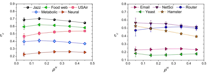
IX. DEPENDENCE OF σc ON THE SIZE OF PERTURBATION SET pH
We have shown how σc is related to the predictability of empirical networks in the main text. The calculation of σc relies on a structural perturbation of the given network. To confirm the relevance of σc in revealing the inherent link predictability of networks, we show that σc is not affected by the size of perturbation set EH. We investigate the dependence of σcon the ratio of the perturbation set ∆E. We change pHfrom 0.05 to 0.45 and find that the differences in σcare relatively small, see the results for ten real-world networks in Fig. S3. Note that σcvaries slowly and steadily with pH, indicating that σc is a robust metric for different sizes of perturbation sets. In practice, therefore, we can select approximately pH of links from the given network to calculate σc. Since σc is not sensitive to the size of ∆E, we can use σc as a metric of link predictability of the network.
0.0 0.1 0.2 0.3 0.4 0.5 0.2 0.3 0.4 0.5 0.6 0.7 0.8 0.9 c p H
Jazz Food web USAir
Metabolic Neural 0.0 0.1 0.2 0.3 0.4 0.5 0.1 0.2 0.3 0.4 0.5 0.6 0.7 0.8 c p H
Email NetSci Router
Yeast Hamster
FIG. S3. (Color online). Dependence of network consistency on the size of perturbation set. The standard deviation is show as the Y-error bar. Each point is obtained by averaging over 100 realizations.
0 5 10 15 20 0.00 0.01 0.02 0.03 0.04 0.05 0.06 0.07 0.08 0.09 0.10 c step PA PA-Random
FIG. S4. The structural consistency for an artificial evolving network. This initial network is constructed by a configuration model with N = 1000,⟨k⟩ = 4 and p(k) ∼ k−3. In each time step, we added 1000 links into the network. The black squares represent the case we continuously using the preferential attachment (PA) mechanism to add new links for 20 time steps, while the red circles stand for the case we change from PA mechanism to random connecting strategy after the 10thtime step.
X. MONITOR THE SUDDEN CHANGES OF EVOLVING NETWORKS WITH σc
The index σc can be used to monitor the changes of network structure during its evolving. Figure S4 gives an example. We artificially build up an evolving model that starting from a configuration network [19] with size N = 1000, average degree ⟨k⟩ = 4 and degree distribution p(k) ∼ k−3. In each step, we will add 1000 new links which are selected according to their popularity (preferential attachment mechanism), that is to say, the probability to add a link connecting nodes (i, j) is proportional to the degree product ki· kj. After the 10thstep (10,000 links are added), we change to random connecting strategy. As shown in figure S4, the structural consistency can well detect this sudden change.
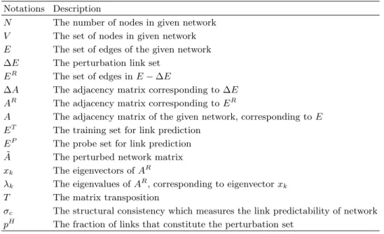
XI. TABLE OF NOTATIONS
TABLE S4. Notations used in the paper. Notations Description
N The number of nodes in given network V The set of nodes in given network E The set of edges of the given network ∆E The perturbation link set
ER The set of edges in E− ∆E
∆A The adjacency matrix corresponding to ∆E AR The adjacency matrix corresponding to ER
A The adjacency matrix of the given network, corresponding to E ET The training set for link prediction
EP The probe set for link prediction ˜
A The perturbed network matrix xk The eigenvectors of AR
λk The eigenvalues of AR, corresponding to eigenvector xk
T The matrix transposition
σc The structural consistency which measures the link predictability of network
pH The fraction of links that constitute the perturbation set
[1] MacArthur BD, S´anchez-Garc´ıa RJ (2009) Spectral characteristics of network redundancy. Phys Rev E 80(2):026117. [2] Hanely JA, McNeil BJ (1983) A method of comparing the areas under receiver operating characteristic curves derived
from the same cases. Radiology 148(3):839-843.
[3] Herlocker JL, Konstann JA, Terveen K, Riedl JT (2004) Evaluating collaborative filtering recommender systems. ACM Trans Inf Syst 22(1):5-53.
[4] Gleiser P, Danon L (2003) Community structure in Jazz. Advances in complex systems 6(04):565.
[5] Duch J, Arenas A (2005) Community detection in complex networks using extremal optimization. Phys Rev E 72(2):027104. [6] Watts DJ, Strogatz SH (1998) Collective dynamics of ’small-world’ networks. Nature 393(6684):440-442.
[7] http://vlado.fmf.uni-lj.si/pub/networks/data/
[8] Ulanowicz RE, Bondavalli C, Egnotovich MS (1998) Network Analysis of Trophic Dynamics in South Florida Ecosystem, FY 97: The Florida Bay Ecosystem. Technical report CBL:98-123. http://www.cbl.umces.edu/ atlss/FBay701.html [9] konect:2013:petster-friendships-hamster, Hamsterster friendships unique network dataset – KONECT, (2013).
http://konect.uni-koblenz.de/networks/petster-friendships-hamster
[10] Newman MEJ (2006) Finding community structure in networks using the eigenvectors of matrices. Phys Rev E 74(3):036104. [11] Sun SW, Ling LJ, Zhang N, Li GJ, Chen RS (2003) Topological structure analysis of the protein-protein interaction
network in budding yeast. Nucleic Acids Research 31(9):2443-2450
[12] Guimer`a R, Danon L, Diaz-Guilera A, Giralt F, Arenas A (2003) Self-similar community structure in a network of human interactions. Phys Rev E 68(6):065103.
[13] Spring N, Mahajan R, Wetherall D, Anderson T (2004) Measuring ISP topologies with Rocketfuel. IEEE/ ACM Trans Networking 12(1):2-16.
[14] Leskovec J, Kleinberg J, Faloutsos C (2007) Graph evolution: Densification and shrinking diameters. ACM Transactions on Knowledge Discovery from Data (TKDD) 1(1):2. (http://konect.uni-koblenz.de/networks/ca-cit-HepTh)
[15] Viswanath B, Mislove A, Cha M, Gummadi KP (2009) On the evolution of user interaction in Facebook. In Proc. Workshop on Online Social Networks, pp 37-42. (http://konect.uni-koblenz.de/networks/facebook-wosn-wall)
[16] Klimt B, Yang Y (2004) The Enron corpus: A new dataset for email classification research. In Proc. European Conf. on Machine Learning, pp 217-226. (http://konect.uni-koblenz.de/networks/enron)
[17] Newman MEJ (2002) Assortative mixing in networks. Phys Rev Lett 89:208701.
[18] Leskovec J, Faloutsos C (2006) Sampling from Large Graphs. Proceedings of the 12th ACM SIGKDD International Con-ference on Knowledge Discovery and Data Mining(ACM, New York), pp 631-636.
[19] Catanzaro M, Boguna M, Pastor-Satorras R (2005) Generation of uncorrelated random scale-free networks. Phys Rev E 71(2):027103.