HAL Id: hal-00015778
https://hal.archives-ouvertes.fr/hal-00015778v2
Submitted on 7 May 2013
HAL is a multi-disciplinary open access
archive for the deposit and dissemination of sci-entific research documents, whether they are pub-lished or not. The documents may come from teaching and research institutions in France or abroad, or from public or private research centers.
L’archive ouverte pluridisciplinaire HAL, est destinée au dépôt et à la diffusion de documents scientifiques de niveau recherche, publiés ou non, émanant des établissements d’enseignement et de recherche français ou étrangers, des laboratoires publics ou privés.
Bias-reduced extreme quantiles estimators of Weibull
distributions
Jean Diebolt, Laurent Gardes, Stephane Girard, Armelle Guillou
To cite this version:
Jean Diebolt, Laurent Gardes, Stephane Girard, Armelle Guillou. Bias-reduced extreme quantiles estimators of Weibull distributions. Journal of Statistical Planning and Inference, Elsevier, 2008, 138 (5), pp.1389-1401. �10.1016/j.jspi.2007.04.025�. �hal-00015778v2�
BIAS-REDUCED EXTREME QUANTILE ESTIMATORS OF WEIBULL TAIL-DISTRIBUTIONS
Jean Diebolt(1), Laurent Gardes(2), St´ephane Girard(2)and Armelle Guillou(3) (1)CNRS, Universit´e de Marne-la-Vall´ee
´
Equipe d’Analyse et de Math´ematiques Appliqu´ees 5, boulevard Descartes, Batiment Copernic
Champs-sur-Marne
77454 Marne-la-Vall´ee Cedex 2, France (2)INRIA Rhˆone-Alpes, team Mistis,
Inovall´ee, 655, av. de l’Europe, Montbonnot, 38334 Saint-Ismier cedex, France
(3)Universit´e Paris VI
Laboratoire de Statistique Th´eorique et Appliqu´ee Boˆıte 158
175 rue du Chevaleret 75013 Paris, France
Abstract. In this paper, we consider the problem of estimating an extreme quantile of a Weibull tail-distribution. The new extreme quantile estimator has a reduced bias compared to the more classical ones proposed in the literature. It is based on an exponential regression model that was introduced in Diebolt et al. (2008). The asymptotic normality of the extreme quantile estimator is established. We also introduce an adaptive selection procedure to determine the number of upper order statistics to be used. A simulation study as well as an application to a real data set are provided in order to prove the efficiency of the above mentioned methods.
Key words and phrases. Weibull tail-distribution, extreme quantile, bias-reduction, least-squares approach, asymptotic normality.
1
Introduction
Let X1, ..., Xn be a sequence of independent and identically distributed (i.i.d.) random
variables with distribution function F. In the present paper, we assume that F is a Weibull tail-distribution, which means that
1− F(x) = exp(−H(x)) with H−1(x) := inf{t : H(t) ≥ x} = xθℓ(x), (1) where θ > 0 denotes the Weibull tail-coefficient and ℓ is a slowly varying function at infinity satisfying
ℓ(λx)
ℓ(x) −→ 1, as x → ∞, for all λ > 0. (2)
Based on the limited sample X1, ..., Xn, the question is how to obtain a good estimate
for a quantile of order 1− pn, pn→ 0 defined by
xpn = inf{y : F(y) ≥ 1 − pn},
such that the quantile to be estimated is situated on the border of or beyond the range of the data. Extrapolation outside the sample occurs for instance in reliability (Ditlevsen, 1994), hydrology (Smith, 1991), and finance (Embrechts et al., 1997). Beirlant et al. (1996) investigated this estimation problem and proposed the following estimator of xpn:
expn =Xn−kn+1,n à log(1/pn) log(n/kn) !eθn , (3)
where X1,n ≤ ... ≤ Xn,n denote the order statistics associated to the original sample and
e
θnis an estimator of θ. One can use for instance the estimator introduced in Diebolt et
al. (2008): e θn= 1 kn kn X i=1
i log(n/i)¡log(Xn−i+1,n)− log(Xn−i,n)¢. (4) We refer to Gardes and Girard (2005) for a study of the properties of (3). In the preceding equations, kndenotes an intermediate sequence, i.e. a sequence such that kn→ ∞ and
kn/n → 0 as n → ∞. See Broniatowski (1993), Beirlant et al. (1995, 1996), Girard
(2004), and Gardes and Girard (2006,2008) for other contributions to the estimation of θ and Beirlant et al. (2006) for Local Asymptotic Normality (LAN) results. Denoting τn = log(1/pn)/ log(n/kn), the estimator (3) can be rewritten as
expn =Xn−kn+1,nτ
e θn
n .
It appears that the extreme quantile of order 1− pn is estimated through an ordinary
quantile of order 1− kn/n with a multiplicative correction τeθnn.
It will appear in the next section that expn exhibits a bias depending on the rate of
convergence to 1 of the ratio of the slowly varying function ℓ in (2). In order to quantify this bias, a second-order condition is required. This assumption can be expressed as follows:
Assumption(Rℓ(b, ρ)). There exists a constant ρ < 0 and a rate function b satisfying b(x)→ 0 as x→ ∞, such that for all ε > 0 and 1 < A < ∞, we have
sup λ∈[1,A] ¯¯ ¯¯ ¯¯log(ℓ(λx)/ℓ(x))b(x)Kρ(λ) − 1 ¯¯ ¯¯
with Kρ(λ) =R1λtρ−1dt.
It can be shown that necessarily |b| is regularly varying with index ρ (see e.g. Geluk and de Haan, 1987). In this paper, we focus on the case where the convergence (2) is slow, and thus when the bias term in eθnand therefore inexpn is large. This situation is
described by the following assumption:
x|b(x)| → ∞ as x → ∞, (5)
which is fulfilled by Gamma, Gaussian and D distributions, see Table 1. The D distribution is an adaptation of Hall’s class (Hall and Welsh, 1985) to the framework of Weibull tail-distributions, see the appendix for its definition. The methodology that we propose in order to reduce the bias ofexpn is to use the following regression model
proposed by Diebolt et al. (2008) for the log-spacings of upper order statistics: Zj := j log¡n/j¢ ³log(Xn−j+1,n)− log(Xn−j,n)
´ = Ã θ + b¡log (n/kn)¢ Ã log(n/kn) log(n/j) !! fj+oP¡b¡log (n/kn)¢¢, (6) for 1 ≤ j ≤ kn, where ( f1, ..., fkn) is a vector of independent and standard
exponen-tially distributed random variables and the oP−term is uniform in j. This exponential regression model is similar to the ones proposed by Beirlant et al. (1999, 2002) and Feuerverger and Hall (1999) in the case of Pareto-type distributions. The model (6) allows us to generate bias-corrected estimates bθn for θ through a Least-Square (LS)
estimation of θ and b(log(n/kn)). The resulting LS estimates are then the following:
b θn =Zkn−bb ¡ log(n/kn)¢xkn bb¡log(n/kn)¢= kn X j=1 (xj− xkn)Zj ,Xkn j=1 (xj− xkn) 2
where xj = log(n/kn)/log(n/j), xkn =
1 kn Pkn j=1xj and Zkn = 1 kn Pkn j=1Zj. The asymptotic
normality of the LS-estimator bθnis established in Diebolt et al. (2008). Now, in order
to refineexpn, we can use the additional information about the slowly varying function
ℓ that is provided by the LS-estimates for θ and b. To this aim, condition (Rℓ(b, ρ)) is used to approximate the ratio F−1(1− p
n)/Xn−kn+1,n, noting that
Xn−kn+1,n
d
=F−1(Un
−kn+1,n),
with U1,n≤ ... ≤ Un,nthe order statistics of a uniform (0, 1) sample of size n,
xpn Xn−kn+1,n d = F −1(1− p n) F−1(Un −kn+1,n) = (− log(pn)) θ (− log(1 − Un−kn+1,n))θ ℓ(− log(pn)) ℓ(− log(1 − Un−kn+1,n)) d = (− log(pn)) θ (− log(Ukn,n))θ ℓ(− log(pn)) ℓ(− log(Ukn,n))
≃ Ã log(1/pn) log(n/kn) !θ exp b¡log(n/kn)¢ ³log(1/pn) log(n/kn) ´ρ − 1 ρ .
The last step follows by replacing Ukn,n with kn/n. Hence, we arrive at the following
estimator for extreme quantiles
bxpn =Xn−kn+1,n à log(1/pn) log(n/kn) !bθn exp bb¡log(n/kn)¢ ³log(1/pn) log(n/kn) ´bρn − 1 b ρn , or equivalently, bxpn =Xn−kn+1,nτ b θn n exp ³ bb(log(n/kn))Kbρ n(τn) ´ .
Here, bρn is an arbitrary estimator of ρ. It will appear in the next section (see
Theo-rem 1(ii)) that, if τnconverges to a constant value τ > 1, one can even choosebρn = ρ#a
constant value, for instance the canonical value ρ# = −1, as suggested by Feuerverger and Hall (1999). Note that the estimator (3) can be seen as a particular case ofbxpn
ob-tained by neglecting the bias-term. In the following, we use the LS-estimators of θ and b defined previously. The study of the asymptotic properties of the extreme quantile estimatorsbxpn andexpn is the aim of Section 2. An adaptive selection procedure for knis
also proposed. A simulation study as well as a real data set are provided in Sections 3 and 4. Proofs are postponed to Section 5.
2
Bias-reduced extreme quantile estimator
The asymptotic normality of our bias-reduced extreme quantile estimatorbxpn is
estab-lished in the following theorem.
Theorem 1 Suppose (1) holds together with (Rℓ(b, ρ)) and (5). We assume that
kn→ ∞, √ kn log(n/kn) b¡log(n/kn)¢ → λ ∈ R, (7) and if λ = 0, √ kn log(n/kn) → ∞ and log2(kn) log(n/kn) → 0. (8) Under the additional condition that
|bρn− ρ| log(τn) = OP(1), (9) we have (i) if τn→ ∞ √ kn log(n/kn) log(τn) ³ log(bxpn)− log(xpn) ´ d −→ N(0, θ2),
(ii) if τn→ τ, τ > 1, and if we replace bρnby a canonical choice ρ# < 0, then
√ kn log(n/kn) ³ log(bxpn)− log(xpn) ´ d −→ N³λµ(τ), θ2σ2(τ)´,
with σ2(τ) = ³Kρ#(τ)− log(τ) ´2 , and µ(τ) =³Kρ#(τ)− Kρ(τ) ´ .
In the following remark we provide some possible choices for the sequences (kn) and
(pn).
Remark 1 Suppose (1) holds together with (Rℓ(b, ρ)) and (5). Then, choosing
kn= Ã λ log(n) b(log(n)) !2 , λ , 0, pn=n−τ, τ > 1, andbρn = ρ#< 0,
Theorem 1(ii) applies and thus 1 b(log(n)) ³ log(bxpn)− log(xpn) ´ d −→ N Ã µ(τ), µθ λ ¶2 σ2(τ) ! . Clearly, the faster b converges to 0, the fasterbxpn converges to xpn.
As a comparison, one can establish similar results forexpn.
Theorem 2 Suppose (1) holds together with (Rℓ(b, ρ)) and (5). We assume that kn→ ∞,
p
knb(log(n/kn))→ λ ∈ R, lim inf τn> 1,
and if λ = 0, log(kn)/ log(n)→ 0, we have:
√ kn
log(τn)
log(expn)− log(xpn)− b(log(n/kn))
log(τkn n) kn X j=1 Ã log(n/j) log(n/kn) !ρ − Kρ(τn) −→ N(0, θd 2). The next corollary allows an asymptotic comparison ofbxpn andexpn.
Corollary 1 Under the assumptions of Theorem 2, we have
(i) if τn→ ∞ √ kn log(τn) ³ log(expn)− log(xpn) ´ d −→ N(λ, θ2), (ii) if τn→ τ, τ > 1, then p kn ³ log(expn)− log(xpn) ´ d −→ N³λ ˜µ(τ), θ2˜σ2(τ)´, with ˜σ2(τ) = log2(τ), and ˜µ(τ) =³log(τ)− Kρ(τ)´.
In the situation where τn → ∞, clearly log(bxpn) is asymptotically unbiased whereas
log(expn) is biased. When τn→ τ, τ > 1 both estimates are asymptotically biased but the
bias of log(bxpn) can be smaller than the one of log(expn) if ρ
Let us now introduce the empirical adapted Asymptotic Mean Squared Error (AMSE∗) ofexpn defined as AMSE∗(expn) = Asymptotic E ³ log(expn)− log(xpn) ´2 .
Note that we use an adapted version of the AMSE since it takes into account the fact that the distribution of the quantile estimators is found to be closer to a lognormal distribution than to the asymptotic normal distribution. This is classical in the literature, see for instance Matthys et al. (2004). As a consequence of Theorem 2, we have
AMSE∗(expn) = θ 2log 2 (τn) kn +b2(log(n/kn)) log(τkn n) kn X j=1 Ã log(n/j) log(n/kn) !ρ − Kρ(τn) 2 . (10) We can now take benefit of the estimation of b(log(n/kn)) by estimating the AMSE∗
given in (10) by: [ AMSE∗(exp n) = (bθn) 2log 2 (τn) kn + (bb(log(n/kn)))2 log(τkn n) kn X j=1 Ã log(n/j) log(n/kn) !−1 + τ−1n − 1 2 . Note that, in the latter formula, we replaced ρ by a canonical choice (ρ =−1) instead of estimating this parameter. In fact, this second-order parameter is difficult to estimate in practice, and we can easily check by simulations that fixing its value does not influence much the result (see e.g. Beirlant et al., 1999, 2002 or Feuerverger and Hall, 1999). Then, the intermediate sequence kncan be selected by minimizing the previous quantity:
ˆkn= arg min kn
[ AMSE∗(exp
n).
This adaptive procedure for selecting the number of upper order statistics is in the same spirit as the one proposed by Matthys et al. (2004) in the case of the Weissman estimator (Weissman, 1978). In order to illustrate the usefulness of the bias reduction and of the selection procedure, we provide a simulation study in the next section.
3
A small simulation study
First, the finite sample performance of the estimatorsexpn andbxpn are investigated on 4
different distributions: |N(0, 1)|, Γ(0.25, 0.25), D(1, 0.5) and W(0.25, 0.25). It is shown in Gardes and Girard (2005) that expn gives better results than the other approaches
(Hosking and Wallis, 1987; Breiman et al., 1990; Beirlant et al., 1995). This explains why bxpn is only compared to the estimatorexpn. In the following, we take pn := pn(τ) = n−τ
with τ = 2 and 4 and we choosebρn = −1. We simulate N = 500 samples (Xn,i)i=1,...,N of
size n = 500. On each sample (Xn,i), the estimatesbxpn(τ),i, are computed for τ = 2, 4 and
for kn = 2, . . . , 360. We present the plots obtained by drawing the points
(kn, medi(log(bxpn(τ),i))) for τ = 2 and 4,
where medi(log(bxpn(τ),i)) is the median value of log(bxpn(τ),i), i = 1, . . . , N. We also present
the associated MSE plots kn, 1 N N X i=1 ³
log(bxpn(τ),i)− log(xpn(τ))
´2
The same procedure is achieved for the estimatorexpn. Results are presented on figures 1–
4. For the|N(0, 1)|, Γ(0.25, 0.25) and D(1, 0.5) distributions, the bias of log(bxpn) is smaller
than the one of log(expn). Let us highlight that, for the latter distribution, a significant bias
reduction is obtained althoughbρn ,ρ. Moreover, bias reduction is usually associated
with an increase in variance. However, as illustrated in panel (b) of figures 1–4, our estimator bxpn is still competitive in an adapted MSE sense. Note that for the
W(0.25, 0.25) distribution, Theorem 1 does not apply since xb(x) = 0. In this case, the behavior of log(expn) is slightly better.
Second, we investigate the behavior of the adaptive procedure for selecting the number of upper order statistics inexpn. For i = 1, . . . , N and τ = 2, 4, we denote by
c kesti
n,i = arg mink
n∈[1,n]
[ AMSE∗(exp
n(τ),i),
the value selected on the sample (Xn,i). As a comparison, we introduce the value that
would be obtained by minimizing the true AMSE∗: koptn = arg min
kn∈[1,n]
AMSE∗(expn(τ)).
Figures 5–8 contain the paired boxplots of the log-quantile estimators log(expn(τ),i) at the
adaptively selected values ckesti
n,i on the right and at the sample fraction k opt
n with smallest
AMSE∗on the left. The horizontal line indicates the true value of log(x
pn). The method
proposed for the adaptive choice of kn, while not achieving the goal of minimizing
the MSE, does lead to quantile estimators that exhibit good bias properties while the variance is inflated in comparison to the asymptotically optimal values.
4
Real data
Here, the good performance of the adaptive selection procedure is illustrated through the analysis of extreme events on the Nidd river data set. This data set is standard in extreme value studies (see e.g. Hosking and Wallis, 1987, or Davison and Smith, 1990.) It consists in 154 exceedances of the level 65 m3s−1by the river Nidd (Yorkshire, England) during the period 1934-1969 (35 years). In environmental studies, the most common quantity of interest is the N-year return level, defined as the level which is exceeded on average once in N years. Here, we focus on the estimation of the 50- and 100- year return levels. According to Hosking and Wallis (1987), the Nidd data may reasonably be assumed to come from a distribution in the Gumbel maximum domain of attraction. This result was confirmed in Diebolt et al. (2008) who have shown that one could consider Weibull tail-distributions as a possible model for such data. The Weibull tail-coefficient is estimated at 0.91. We obtained 321.5m3s−1 as an estimation of the 50-year return level and 359m3s−1 as an estimation of the 100-year return level. Note that these results are in accordance with the results obtained by profile-likelihood or Bayesian methods, see Diebolt et al. (2005) or Davison and Smith (1990).
5
Proofs
Proof of Theorem 1. We decompose our quantile estimator as follows: log(bxpn)− log(xpn) = log(Xn−kn+1,n) + bθnlog(τn)
+ bb¡log(n/kn)¢Kbρ n(τn)− log ³ (− log(pn))θℓ(− log(pn)) ´ d = θ©log¡− log¡Uk n,n ¢¢ − log log(n/kn)ª + ³bθn− θ´log(τn) + ©log ℓ¡− log¡Uk n,n ¢¢ − log ℓ¡log(n/kn)¢ª
+ nlog ℓ¡log(n/kn)¢− log ℓ¡− log(pn)¢+b¡log(n/kn)¢Kρ(τn)o + ³bb¡log(n/kn)¢− b¡log(n/kn)¢´K b ρn(τn) + b¡log(n/kn)¢ nK b ρn(τn)− Kρ(τn) o := 6 X j=1 Bj,kn.
We successively discuss each of the terms Bj,kn, j = 1, ..., 6. First concerning B1,kn, remark
that log¡− log(Ukn,n) ¢ − log log(n/kn) d = log à Tn−kn+1,n log(n/kn) ! ,
where Tj,n denotes the order statistics from an i.i.d. standard exponential sample of
size n. Since it is well known that p kn¡Tn−kn+1,n− log(n/kn) ¢ d −→ N(0, 1), (11) we clearly have √ kn log(n/kn) log(τn) B1,kn =OP Ã 1 log2(n/kn) log τn ! =oP(1). (12)
Remark now that √ kn log(n/kn) log(τn) B2,kn = √ kn log(n/kn) ³ b θn− θ ´ d −→ N(0, θ2), (13)
by Theorem 3.1 in Diebolt et al. (2008). Next, using (Rℓ(b, ρ)) and (11), we get B3,kn d = log à ℓ(Tn−kn+1,n) ℓ(log(n/kn)) ! = Kρ à Tn−kn+1,n log(n/kn) ! b(log(n/kn))(1 + oP(1)) = à Tn−kn+1,n log(n/kn) − 1 ! b(log(n/kn))(1 + oP(1)) = OP √b(log(n/kk n)) nlog(n/kn) , (14) so that under (7), √ kn log(n/kn) log(τn) B3,kn =OP √k 1 nlog(n/kn) log(τn) =oP(1). (15)
Next, under (Rℓ(b, ρ)) one has (for a suitably chosen b) that for all ǫ > 0 (see Drees, 1998, Lemma 2.1) sup t>1 t−(ǫ+ρ)¯¯¯¯¯log ℓ(tx)− log ℓ(x) b(x) − Kρ(t) ¯¯ ¯¯ ¯ −→ 0. Hence, we conclude, choosing ǫ <−ρ, that
¯¯ ¯¯ ¯ B4,kn b(log(n/kn)) ¯¯ ¯¯ ¯ = ¯¯ ¯¯ ¯¯log ℓ ¡
log(n/kn)¢− log ℓ(τnlog(n/kn))
b(log(n/kn))
+Kρ(τn) ¯¯ ¯¯
¯¯ −→ 0, (16)
which implies that, under (7), we have √ kn log(n/kn) log(τn) B4,kn =o à 1 log(τn) ! =o(1). (17)
Next, we can check that, according to (6), B5,kn =Kbρn(τn) 1 kn kn X j=1 βj,n( fj− 1), where βj,n := (xj− xkn)(θ + b(log(n/kn))xj) 1 kn Pkn i=1(xi− xkn)2 .
A direct application of Lyapounov’s theorem, combined with Lemma 7.3 in Diebolt et al. (2008) yields √ kn log(n/kn) 1 kn kn X j=1 βj,n( fj− 1) d −→ N(0, θ2). Therefore √ kn log(n/kn) log(τn) B5,kn = Kbρn(τn) log(τn) ξ1,n with ξ1,n−→ N(0, θd 2). (18)
Finally, following the method of proof of Lemma 1 in de Haan and Rootz´en (1993), we
find that ¯¯ ¯¯ ¯ Z τn 1 sρ−1(sbρn−ρ− 1) ds − (bρ n− ρ) Z τn 1 sρ−1 log(s) ds¯¯¯¯¯ ≤ |bρn− ρ| Z τn 1 sρ−1 log(s) (s|bρn−ρ|− 1) ds ≤ |bρn− ρ| ÃZ τn 1 sρ−1 log(s) ds! ³τ|bρn−ρ| n − 1 ´ , where the first inequality comes from the fact that¯¯¯ex−1
x − 1¯¯¯ ≤ e|x|− 1. Hence √ kn log(n/kn) log(τn) B6,kn = √ kn log(n/kn) b¡log(n/kn)¢ × ¡bρn− ρ¢ R τn 1 x ρ−1 log(x) dx log(τn) n 1 + O³τ|bρn−ρ| n − 1 ´o .
If τn→ ∞, this implies that bρn
P
→ ρ by the assumption (9) and therefore √
kn
log(n/kn) log(τn)
B6,kn =oP(1). (19)
Combining (12), (13) and (15) with (17)-(19), Theorem 1(i) follows. If τn → τ, τ > 1,
then the normalization factor log(τn)→ log(τ) , 0 can be omitted in (12), (15) and (17)
while preserving the negligeability of these terms. Besides, we can replacebρnwith any
canonical choice, for instance ρ# < 0, and therefore √ kn log(n/kn) B6,kn = √ kn log(n/kn) b¡log(n/kn)¢ ³Kρ#(τn)− Kρ(τn) ´ −→ λµ(τ) := λ³Kρ#(τ)− Kρ(τ) ´ . (20)
The limiting distribution is then given by (13) and (18) with a bias term due to (20). To conclude with the second part of our Theorem 1, we have to establish the limiting distribution of Un := √ knKρ#(τn) log(n/kn) ³ bb¡log(n/kn)¢− b¡log(n/kn)¢´+ √ knlog(τn) log(n/kn) ³ b θn− θ ´ . To this aim, remark that
Un = k−12 n log(n/kn) kn X j=1 ωj,n( fj− 1) + oP(1), where ωj,n = βj,nKρ#(τn) + αj,nlog(τn) and αj,n = ³ θ + b¡log(n/kn)¢xj ´ 1 − 1 xj− xkn kn Pkn i=1(xi− xkn)2 xkn . Using Lemma 7.3 in Diebolt et al. (2008), direct computations lead to
kn X j=1 Var³ωj,n( fj− 1) ´ = kn X j=1 ω2j,n ∼ θ2¡log(n/kn)¢2 knσ2(τ) and kn X j=1 E³ωj,n( fj− 1)´4 = 9 kn X j=1 ω4j,n ∼ Ckn ¡log(n/kn)¢4,
where C is a suitable constant. Therefore a direct application of Lyapounov’s theorem yields
Un d
−→ N³0, θ2σ2(τ)´,
Proof of Theorem 2. We have:
log(expn)− log(xpn)− b(log(n/kn)) log(τn)
1 kn kn X j=1 Ã log(n/j) log(n/kn) !ρ +b(log(n/kn))τ ρ n− 1 ρ = θ{log(− log(Uk n,n))− log log(n/kn)} + eθn− θ − b(log n/kn) 1 kn kn X j=1 Ã log(n/j) log(n/kn) !ρ log(τn) + {log ℓ(− log(Uk n,n))− log ℓ(log(n/kn))} + (
log ℓ(log(n/kn))− log ℓ(− log(pn)) + b(log(n/kn))
τρn− 1 ρ ) := B1,kn+B7,kn +B3,kn +B4,kn. From (12), we have √ kn log(τn) B1,kn =OP Ã 1 log(n/kn) log(τn) ! =oP(1),
and Theorem 2.2 in Diebolt et al. (2008) states that √ kn log(τn) B7,kn d −→ N(0, θ2). From (14), we have B3,kn =OP √b(log(n/kk n)) nlog(n/kn) , and thus √knb(log(n/kn))→ λ ∈ R entails
√ kn log(τn) B3,kn =OP √k 1 nlog(n/kn) log(τn) =oP(1). Finally, (16) implies that
B4,kn =oP(b(log(n/kn))),
which, combined with √knb(log(n/kn))→ λ ∈ R yields
√ kn log(τn) B4,kn =oP Ã 1 log(τn) ! =oP(1),
which achieves the proof of Theorem 2. ⊔⊓
Appendix
Diebolt et al. (2008) introduced the class of distributions D(α, β) with distribution function given by
1− F(x) = exp(−H(x)) where H−1(x) := x1/α(1 + x−β),
α and β being two parameters such that 0 < α, 0 < β < 1 and αβ ≤ 1. Under these conditions, the above class of distributions fulfill assumptions (1) with (Rℓ(b, ρ)) and
(5) where θ = 1/α, ρ =−β, ℓ(x) = 1 + x−βand b(x) =−βx−β. It is thus possible to obtain distributions with arbitrary θ > 0 and −1 < ρ < 0. These results are summarized in Table 1.
Acknowledgement
The authors are grateful to the referees for a careful reading of the paper that led to significant improvements of the earlier draft.
References
[1] Beirlant, J., Bouquiaux, C., Werker, B., (2006), Semiparametric lower bounds for tail index estimation, Journal of Statistical Planning and Inference, 136, 705–729. [2] Beirlant, J., Broniatowski, M., Teugels, J.L., Vynckier, P., (1995), The mean residual
life function at great age: Applications to tail estimation, Journal of Statistical Planning and Inference, 45, 21–48.
[3] Beirlant, J., Dierckx, G., Goegebeur, Y., Matthys, G., (1999), Tail index estimation and an exponential regression model, Extremes, 2, 177–200.
[4] Beirlant, J., Dierckx, G., Guillou, A., Starica, C., (2002), On exponential representa-tions of log-spacings of extreme order statistics, Extremes, 5, 157–180.
[5] Beirlant, J., Teugels, J., Vynckier, P., (1996), Practical analysis of extreme values, Leuven university press, Leuven.
[6] Breiman, L., Stone, C. J., Kooperberg, C. (1990), Robust confidence bounds for extreme upper quantiles, Journal of Computational Statistics and Simulation, 37, 127– 149.
[7] Broniatowski, M., (1993), On the estimation of the Weibull tail coefficient, Journal of Statistical Planning and Inference, 35, 349–366.
[8] Davison, A., Smith, R., (1990), Models for exceedances over high thresholds, Journal of the Royal Statistical Society Ser. B, 52, 393–442.
[9] Diebolt, J., El-Aroui, M., Garrido, M., Girard, S., (2005), Quasi-conjugate Bayes estimates for GPD parameters and application to heavy tails modelling, Extremes,
8, 57–78.
[10] Diebolt, J., Gardes, L., Girard, S., Guillou, A., (2008), Bias-reduced estimators of the Weibull-tail coefficient, Test, 17, 311–331.
[11] Ditlevsen, O., (1994), Distribution Arbitrariness in Structural Reliability, Structural Safety and Reliability, 1241–1247, Balkema, Rotterdam.
[12] Drees, H., (1998), On smooth statistical tail functionals, Scandinavian Journal of Statistics, 25, 187–210.
[13] Embrechts, P., Kl ¨uppelberg, C., Mikosch, T., (1997), Modelling extremal events, Springer.
[14] Feuerverger, A., Hall, P., (1999), Estimating a Tail Exponent by Modelling Depar-ture from a Pareto Distribution, Annals of Statistics, 27, 760–781.
[15] Gardes, L., Girard, S., (2005), Estimating extreme quantiles of Weibull tail-distributions, Communication in Statistics - Theory and Methods, 34, 1065–1080. [16] Gardes, L., Girard, S., (2006), Comparison of Weibull tail-coefficient estimators,
REVSTAT - Statistical Journal, 4, 163–188.
[17] Gardes, L., Girard, S., (2008), Estimation of the Weibull tail-coefficient with linear combination of upper order statistics, Journal of Statistical Planning and Inference,
138, 1416–1427.
[18] Geluk, J.L., de Haan, L., (1987), Regular Variation, Extensions and Tauberian Theorems, Math Centre Tracts, 40, Centre for Mathematics and Computer Science, Amsterdam.
[19] Girard, S., (2004), A Hill type estimate of the Weibull tail-coefficient, Communication in Statistics - Theory and Methods, 33, 205–234.
[20] de Haan, L., Rootz´en, H., (1993), On the estimation of high quantiles, Journal of Statistical Planning and Inference, 35, 1–13.
[21] Hall, P., Welsh, A.H., (1985), Adaptive estimates of parameters of regular variation, Annals of Statistics, 13, 331–341.
[22] Hosking, J., Wallis, J., (1987), Parameter and quantile estimation for the generalized Pareto distribution, Technometrics, 29, 339–349.
[23] Matthys, G., Delafosse, E., Guillou, A., Beirlant, J., (2004), Estimating catastrophic quantile levels for heavy-tailed distributions, Insurance Mathematics & Economics,
34, 517–537.
[24] Smith, J., (1991), Estimating the upper tail of flood frequency distributions, Water Resources Research, 23, 1657–1666.
[25] Weissman, I., (1978), Estimation of parameters and large quantiles based on the k largest observations, Journal of the American Statistical Association, 73, 812–815.
Distribution θ b(x) ρ Absolute Gaussian|N|(µ, σ2) 1/2 1 4 log x x −1 Gamma Γ(α , 1, β) 1 (1− α)log x x −1 WeibullW(α, λ) 1/α 0 −∞ D(α, β) 1/α −βx−β −β
0 50 100 150 200 250 300 350 1.6 1.7 1.8 1.9 2.0 2.1 2.2 k Median 0 50 100 150 200 250 300 350 1.6 1.7 1.8 1.9 2.0 2.1 2.2 k Median −−−−−−−−−−−−−−−−−−−−−−−−−−−−−−−−−−−−−−−−−−−−−−−−−−−−−−−−−−−−−−−−−−−−−−−−−−−−−−−−−−−−−−−−−−−−−−−−−−−−−−−−−−−−−−−−−−−−−−−−−−−−−−−−−−−−−−−−−−−−−−−−−−−−−−−−−−−−−−−−−−−−−−−−−−−−−−−−−−−−−−−−−−−−−−−−−−−−−−−−−−−−−−−−−−−−−−−−−−−−−−−−−−−−−−−−−−−−−−−−−−−−−−−−−−−−−−−−−−−−−−−−−−−−−−−−−−−−−−−−−−−−−−−−−−−−−−−−−−−−−−−−−−−−−−−−−−−−−−−−−−−−−−−−−−−−−−−−−−−−−−−−−−−−−−−−−−−−−− 0 50 100 150 200 250 300 350 1.6 1.7 1.8 1.9 2.0 2.1 2.2 k Median + + + + + ++++ +++++++++ ++++++++++++++ +++++++++++++++++++++++++++++++++++++++++++++++++++++++++++++++++++++++++++++++++++++++++++++++++++++++++++++++++++++++++++++++++++++++++++++++++++++++++++++++++++++++++++++++++++++++++++++++++++++++++++++++++++++++++++++++++++++++++++++++++++++++++++++++++++++++++++++++++++++++++++++++++++ 0 50 100 150 200 250 300 350 1.6 1.7 1.8 1.9 2.0 2.1 2.2 k Median ** * * * * * * *** * ** ** ****** * *********************** ********* ***************************************** * ***************************************************************************************** ******************************************************************** ************************************************** ************************************* ***************** 0 50 100 150 200 250 300 350 1.6 1.7 1.8 1.9 2.0 2.1 2.2 k Median ********************************************************************************************************************************************************************************************************************************************************************************************************************************************************************** 0 50 100 150 200 250 300 350 1.6 1.7 1.8 1.9 2.0 2.1 2.2 k Median
(a) Median as a function of kn
0 50 100 150 200 250 300 350 0.000 0.005 0.010 0.015 0.020 k MSE 0 50 100 150 200 250 300 350 0.000 0.005 0.010 0.015 0.020 k MSE + + + + + + + ++ + + ++++ +++ ++++ +++++++++++++++++++++ +++++++++++++++++++++++++++++++++++++++++++++++++++++++++++++++++++++++++++++++++++++++++++++++++++++++++++++++++++++++++++++++++++++++++++++++++++++++++++++++++++++++++++++++++++++++++++++++++++++++++++++++++++++++++++++++++++++++++++++++++++++++++++++++++++++++++++++++++++++++++++++++++++++++++++++++++ 0 50 100 150 200 250 300 350 0.000 0.005 0.010 0.015 0.020 k MSE ** * ** *** *** ** * ** ** ** **** ** ******** * *** * ** ****** ************ *** ****** ******************* ******************* ******************** ************************************************************************************************************************************************* 0 50 100 150 200 250 300 350 0.000 0.005 0.010 0.015 0.020 k MSE (b) MSE as a function of kn
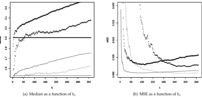
Figure 1: Comparison of log(expn) (τ = 2: continuous line, τ = 4: + + +) and log(bxpn) (τ = 2:
dashed line, τ = 4: ⋆ ⋆ ⋆) for the|N(0, 1)| distribution. The horizontal lines on the left panel
represent the true values of log(xpn) (thin line: τ = 2, thick line: τ = 4).
0 50 100 150 200 250 300 350 8.5 9.0 9.5 10.0 10.5 11.0 11.5 k Median 0 50 100 150 200 250 300 350 8.5 9.0 9.5 10.0 10.5 11.0 11.5 k Median −−−−−−−−−−−−−−−−−−−−−−−−−−−−−−−−−−−−−−−−−−−−−−−−−−−−−−−−−−−−−−−−−−−−−−−−−−−−−−−−−−−−−−−−−−−−−−−−−−−−−−−−−−−−−−−−−−−−−−−−−−−−−−−−−−−−−−−−−−−−−−−−−−−−−−−−−−−−−−−−−−−−−−−−−−−−−−−−−−−−−−−−−−−−−−−−−−−−−−−−−−−−−−−−−−−−−−−−−−−−−−−−−−−−−−−−−−−−−−−−−−−−−−−−−−−−−−−−−−−−−−−−−−−−−−−−−−−−−−−−−−−−−−−−−−−−−−−−−−−−−−−−−−−−−−−−−−−−−−−−−−−−−−−−−−−−−−−−−−−−−−−−−−−−−−−−−−−−−− 0 50 100 150 200 250 300 350 8.5 9.0 9.5 10.0 10.5 11.0 11.5 k Median + + ++ + ++++ +++++++ ++++++++ ++ + +++++++++++++++++++++++++++++++++++++++++++++++++++++++++++++++++++++++++++++++++++++++++++++++++++++++++++++++++++++++++++++++++++++++++++++++++++++++++++++++++++++++++++++++++++++++++++++++++++++++++++++++++++++++++++++++++++++++++++++++++++++++++++++++++++++++++++++++++++++++++++++++++++++++++++++++++++++++++++++++++++++++++++ 0 50 100 150 200 250 300 350 8.5 9.0 9.5 10.0 10.5 11.0 11.5 k Median * * * * * * * * * * *** * *** * * ** * ** * ** * ** * ****** * * ********** * ******************* ********** * ****** * ****************** * **************** * ************************************************ *** ************************************************************************************************************************************************************************************ ** 0 50 100 150 200 250 300 350 8.5 9.0 9.5 10.0 10.5 11.0 11.5 k Median ********************************************************************************************************************************************************************************************************************************************************************************************************************************************************************** 0 50 100 150 200 250 300 350 8.5 9.0 9.5 10.0 10.5 11.0 11.5 k Median
(a) Median as a function of kn
0 50 100 150 200 250 300 350 0 5 10 15 20 k MSE 0 50 100 150 200 250 300 350 0 5 10 15 20 k MSE + + + + + + + ++++++ + + ++++ ++ ++ +++++++++++++++++++++++++++++++++++++++++++++++++++++++++++++++++++++++++++++++++++++++++++++++++++++++++++++++++++++++++++++++++++++++++++++++++++++++++++++++++++++++++++++++++++++++++++++++++++++++++++++++++++++++++++++++++++++++++++++++++++++++++++++++++++++++++++++++++++++++++++++++++++++++++++++++++++++++++++++++++++++ 0 50 100 150 200 250 300 350 0 5 10 15 20 k MSE ****** * * * * * * * * * **** * ** ** ********** ** ** ******* ******* *************** ******** **** *** **************** ******* *********** ******************************** *************************************************************************************************************************** 0 50 100 150 200 250 300 350 0 5 10 15 20 k MSE (b) MSE as a function of kn
Figure 2: Comparison of log(expn) (τ = 2: continuous line, τ = 4: + + +) and log(bxpn) (τ = 2:
dashed line, τ = 4: ⋆ ⋆ ⋆) for theW(0.25, 0.25) distribution. The horizontal lines on the left
0 50 100 150 200 250 300 350 4.0 4.5 5.0 5.5 6.0 6.5 k Median 0 50 100 150 200 250 300 350 4.0 4.5 5.0 5.5 6.0 6.5 k Median −−−−−−−−−−−−−−−−−−−−−−−−−−−−−−−−−−−−−−−−−−−−−−−−−−−−−−−−−−−−−−−−−−−−−−−−−−−−−−−−−−−−−−−−−−−−−−−−−−−−−−−−−−−−−−−−−−−−−−−−−−−−−−−−−−−−−−−−−−−−−−−−−−−−−−−−−−−−−−−−−−−−−−−−−−−−−−−−−−−−−−−−−−−−−−−−−−−−−−−−−−−−−−−−−−−−−−−−−−−−−−−−−−−−−−−−−−−−−−−−−−−−−−−−−−−−−−−−−−−−−−−−−−−−−−−−−−−−−−−−−−−−−−−−−−−−−−−−−−−−−−−−−−−−−−−−−−−−−−−−−−−−−−−−−−−−−−−−−−−−−−−−−−−−−−−−−−−−−− 0 50 100 150 200 250 300 350 4.0 4.5 5.0 5.5 6.0 6.5 k Median + + + +++++ + +++++++++++++ + +++++++++++++++++ +++++++++++++++++++++++++++++++++++++++++++++++++++++++++++++++++++++++++++++++++++++++++++++++++++++++++++++++++++++++++++++++++++++++++++++++++++++++++++++++++++++++++++++++++++++++++++++++++++++++++++++++++++++++++++++++++++++++++++++++++++++++++++++++++++++ 0 50 100 150 200 250 300 350 4.0 4.5 5.0 5.5 6.0 6.5 k Median * * * ** * **** * * ******** * *************** * *** ************************************ ************************************************************************* ******************************************************* *************************** ************************************ ********************************************** ******************* ******************* ***** 0 50 100 150 200 250 300 350 4.0 4.5 5.0 5.5 6.0 6.5 k Median ********************************************************************************************************************************************************************************************************************************************************************************************************************************************************************** 0 50 100 150 200 250 300 350 4.0 4.5 5.0 5.5 6.0 6.5 k Median
(a) Median as a function of kn
0 50 100 150 200 250 300 350 0.0 0.5 1.0 1.5 k MSE 0 50 100 150 200 250 300 350 0.0 0.5 1.0 1.5 k MSE + + + + + ++ + + ++ + +++ ++ ++ + +++++++++++++++ ++++++++++ +++++++++ + ++++++++++++++++++++++++++++++++++++++++++ +++++++++++++ +++++++++++++++++++++++++++++++++++++++ + ++++++++++++++ + ++++++++++++++++++++ + +++++++ + ++++++++++++++++++++++++++ ++++++++++++++++++++ + +++ + ++ + +++++++++ ++++++++++++++++++ 0 50 100 150 200 250 300 350 0.0 0.5 1.0 1.5 k MSE **** *** * * * *** ** * * *** ***** ******* ***** ****** ** * *************** *************** ************************* ****************** ****************************************************************************************** * *********** *************** ************************* ************* **************** 0 50 100 150 200 250 300 350 0.0 0.5 1.0 1.5 k MSE (b) MSE as a function of kn
Figure 3: Comparison of log(expn) (τ = 2: continuous line, τ = 4: + + +) and log(bxpn) (τ = 2:
dashed line, τ = 4: ⋆ ⋆ ⋆) for the Γ(0.25, 0.25) distribution. The horizontal lines on the left panel
represent the true values of log(xpn) (thin line: τ = 2, thick line: τ = 4).
0 50 100 150 200 250 300 350 2.8 3.0 3.2 3.4 k Median 0 50 100 150 200 250 300 350 2.8 3.0 3.2 3.4 k Median + + +++ ++++ +++++ ++++++++++++++++++++++++++++++++++++++++++++++++++++++++++++++++++++++++++++++++++++++++++++++++++++++++++++++++++++++++++++++++++++++++++++++++++++++++++++++++++++++++++++++++++++++++++++++++++++++++++++++++++++++++++++++++++++++++++++++++++++++++++++++++++++++++++++++++++++++++++++++++++++++++++++++++++++++++++++++++++++++++++++++++++++++++ 0 50 100 150 200 250 300 350 2.8 3.0 3.2 3.4 k Median * * * * ** ** ** * * *** **** ** *** * ************* ******* ****** ******************************* ****************************************************************************************************************************************************************************************************************************** ***************************************************** 0 50 100 150 200 250 300 350 2.8 3.0 3.2 3.4 k Median ********************************************************************************************************************************************************************************************************************************************************************************************************************************************************************** 0 50 100 150 200 250 300 350 2.8 3.0 3.2 3.4 k Median −−−−−−−−−−−−−−−−−−−−−−−−−−−−−−−−−−−−−−−−−−−−−−−−−−−−−−−−−−−−−−−−−−−−−−−−−−−−−−−−−−−−−−−−−−−−−−−−−−−−−−−−−−−−−−−−−−−−−−−−−−−−−−−−−−−−−−−−−−−−−−−−−−−−−−−−−−−−−−−−−−−−−−−−−−−−−−−−−−−−−−−−−−−−−−−−−−−−−−−−−−−−−−−−−−−−−−−−−−−−−−−−−−−−−−−−−−−−−−−−−−−−−−−−−−−−−−−−−−−−−−−−−−−−−−−−−−−−−−−−−−−−−−−−−−−−−−−−−−−−−−−−−−−−−−−−−−−−−−−−−−−−−−−−−−−−−−−−−−−−−−−−−−−−−−−−−−−−−− 0 50 100 150 200 250 300 350 2.8 3.0 3.2 3.4 k Median
(a) Median as a function of kn
0 50 100 150 200 250 300 350 0.00 0.01 0.02 0.03 0.04 0.05 0.06 k MSE 0 50 100 150 200 250 300 350 0.00 0.01 0.02 0.03 0.04 0.05 0.06 k MSE + + + + + + ++ + + + + ++ +++ ++ + ++++++++++++++++++++++++++++++++++++++++++++++++++++++++++++++++++++++++++++++++++++++++++++++++++++++++++++++++++++++++++++++++++++++++++++++++++++++++++++++++++++++++++++++++++++++++++++++++++++++++++++++++++++++++++++++++++++++++++++++++++++++++++++++++++++++++++++++++++++++++++++++++++++++++++++++++++++++++++++++++++++++++++ 0 50 100 150 200 250 300 350 0.00 0.01 0.02 0.03 0.04 0.05 0.06 k MSE ** ** **** * * * * ** ** * * * * *** *** * ***** ***** ** ********** ******* *** ******** **** ****** ******************************* ************************************************************************************************ ********************************************************************* 0 50 100 150 200 250 300 350 0.00 0.01 0.02 0.03 0.04 0.05 0.06 k MSE (b) MSE as a function of kn
Figure 4: Comparison of log(expn) (τ = 2: continuous line, τ = 4: + + +) and log(bxpn) (τ = 2:
dashed line, τ = 4: ⋆ ⋆ ⋆) for theD(1, 0.5) distribution. The horizontal lines on the left panel
opt esti 1.2 1.4 1.6 1.8 Log−Quantiles (a) τ = 2 opt esti 1.5 2.0 2.5 Log−Quantiles (b) τ = 4
Figure 5: |N(0, 1)| distribution. Boxplots of log(expn) at the optimal value of kn obtained by
minimizing the true AMSE∗(left), and at the value of knobtained by minimizing the estimated
AMSE∗(right). The horizontal line indicates the true value of log(xpn).
opt esti 5 6 7 8 9 10 Log−Quantiles (a) τ = 2 opt esti 6 8 10 12 14 Log−Quantiles (b) τ = 4
Figure 6: W(0.25, 0.25) distribution. Boxplots of log(expn) at the optimal value of knobtained by
minimizing the true AMSE∗(left), and at the value of knobtained by minimizing the estimated
opt esti 2.5 3.0 3.5 4.0 4.5 5.0 Log−Quantiles (a) τ = 2 opt esti 3 4 5 6 7 Log−Quantiles (b) τ = 4
Figure 7: Γ(0.25, 0.25) distribution. Boxplots of log(expn) at the optimal value of knobtained by
minimizing the true AMSE∗(left), and at the value of knobtained by minimizing the estimated
AMSE∗(right). The horizontal line indicates the true value of log(xpn).
opt esti 2.0 2.5 3.0 3.5 4.0 Log−Quantiles (a) τ = 2 opt esti 2.0 2.5 3.0 3.5 4.0 Log−Quantiles (b) τ = 4
Figure 8: D(1, 0.5) distribution. Boxplots of log(expn) at the optimal value of kn obtained by
minimizing the true AMSE∗(left), and at the value of knobtained by minimizing the estimated