When can temporally focused excitation be axially shifted by dispersion?

(1)

HAL Id: hal-01963755

https://hal.archives-ouvertes.fr/hal-01963755

Submitted on 21 Dec 2018

HAL is a multi-disciplinary open access

archive for the deposit and dissemination of

sci-entific research documents, whether they are

pub-lished or not. The documents may come from

teaching and research institutions in France or

abroad, or from public or private research centers.

L’archive ouverte pluridisciplinaire HAL, est

destinée au dépôt et à la diffusion de documents

scientifiques de niveau recherche, publiés ou non,

émanant des établissements d’enseignement et de

recherche français ou étrangers, des laboratoires

publics ou privés.

When can temporally focused excitation be axially

shifted by dispersion?

B. Leshem, O. Hernandez, E. Papagiakoumou, V. Emiliani, D. Oron

To cite this version:

B. Leshem, O. Hernandez, E. Papagiakoumou, V. Emiliani, D. Oron. When can temporally focused

excitation be axially shifted by dispersion?. Optics Express, Optical Society of America - OSA

Pub-lishing, 2014, 22 (6), pp.7087. �10.1364/oe.22.007087�. �hal-01963755�

(2)

When can temporally focused excitation

be axially shifted by dispersion?

B. Leshem,1,3_{O. Hernandez,}2,3_{E. Papagiakoumou,}2_{V. Emiliani,}2_and

D. Oron1,*

1_{Department of physics of Complex Systems, Weizmann Institute of Science, Rehovot 76100,}

Israel

2_{Wavefront-engineering Microscopy Group, Neurophotonics Laboratory, CNRS UMR 8250,}

Paris Descartes University, 45 rue des Saints-P`eres 75270 Paris Cedex 06, France

3_{Equal contributors}

∗_{dan.oron@weizmann.ac.il}

Abstract: Temporal focusing (TF) allows for axially confined wide-field multi-photon excitation at the temporal focal plane. For temporally focused Gaussian beams, it was shown both theoretically and experimentally that the temporal focus plane can be shifted by applying a quadratic spectral phase to the incident beam. However, the case for more complex wave-fronts is quite different. Here we study the temporal focus plane shift (TFS) for a broader class of excitation profiles, with particular emphasis on the case of temporally focused computer generated holography (CGH) which allows for generation of arbitrary, yet speckled, 2D patterns. We present an analytical, numerical and experimental study of this phenomenon. The TFS is found to depend mainly on the autocorrelation of the CGH pattern in the direction of the beam dispersion after the grating in the TF setup. This provides a pathway for 3D control of multi-photon excitation patterns.

OCIS codes: (090.1995) Digital holography; (170.6900) Three-dimensional microscopy; (320.7110) Ultrafast nonlinear optics.

References and links

1. D. Oron, E. Tal, and Y. Silberberg, “Scanningless depth-resolved microscopy,” Opt. Express 13, 1468–1476 (2005).

2. G. Zhu, J. van Howe, M. E. Durst, W. Zipfel, and C. Xu, “Simultaneous spatial and temporal focusing of fem-tosecond pulses,” Opt. Express 13, 2153–2159 (2005).

3. E. Papagiakoumou, F. Anselmi, A. B`egue, V. de Sars, J. Gl¨uckstad, E. Y. Isacoff, and V. Emiliani, “Scanless two-photon excitation of channelrhodopsin-2,” Nat. Methods 7, 848–854 (2010).

4. A. Vaziri, J. Tang, H. Shroff, and C. V. Shank, “Multilayer three-dimensional super resolution imaging of thick biological samples,” Proc. Natl Acad. Sci. U. S. A. 105, 20221–20226 (2008).

5. E. Y. S. Yew, H. Choi, D. Kim, and P. T. C. So, “Wide-field two-photon microscopy with temporal focusing and hilo background rejection,” in “SPIE BiOS” (International Society for Optics and Photonics, 2011), p. 79031O. 6. E. Papagiakoumou, A. B`egue, B. Leshem, O. Schwartz, B. M. Stell, J. Bradley, D. Oron, and V. Emiliani,

“Func-tional patterned multiphoton excitation deep inside scattering tissue,” Nat. Photonics 7, 274–278 (2013). 7. E. Block, M. Greco, D. Vitek, O. Masihzadeh, D. A. Ammar, M. Y. Kahook, N. Mandava, C. Durfee, and

J. Squier, “Simultaneous spatial and temporal focusing for tissue ablation,” Bio. Opt. Express 4, 831–841 (2013). 8. H. Suchowski, D. Oron, and Y. Silberberg, “Generation of a dark nonlinear focus by spatio-temporal coherent

control,” Opt. Commun. 264, 482–487 (2006).

9. M. E. Durst, G. Zhu, and C. Xu, “Simultaneous spatial and temporal focusing for axial scanning,” Opt. Express 14, 12243–12254 (2006).

10. M. E. Durst, G. Zhu, and C. Xu, “Simultaneous spatial and temporal focusing in nonlinear microscopy,” Opt. Commun. 281, 1796–1805 (2008).

(3)

11. O. Martinez, “3000 times grating compressor with positive group velocity dispersion: Application to fiber com-pensation in 1.3-1.6 µm region,” IEEE J. Quantum Electron. 23, 59–64 (1987).

12. R. W. Gerchberg and W. O. Saxton, “A practical algorithm for the determination of phase from image and diffraction plane pictures,” Optik 35, 237–246 (1972).

13. M. Reicherter, T. Haist, E. U. Wagemann, and H. J. Tiziani, “Optical particle trapping with computer-generated holograms written on a liquid-crystal display,” Opt. Lett. 24, 608–610 (1999).

14. C. Lutz, T. S. Otis, V. de Sars, S. Charpak, D. A. DiGregorio, and V. Emiliani, “Holographic photolysis of caged neurotransmitters,” Nat. Methods 5, 821–827 (2008).

15. P. Wang and R. Menon, “Three-dimensional lithography via digital holography,” in “Frontiers in Optics” (Optical Society of America, 2012).

16. J. E. Curtis, B. A. Koss, and D. G. Grier, “Dynamic holographic optical tweezers,” Opt. Commun. 207, 169–175 (2002).

17. I. Reutsky-Gefen, L. Golan, N. Farah, A. Schejter, L. Tsur, I. Brosh, and S. Shoham, “Holographic optogenetic stimulation of patterned neuronal activity for vision restoration,” Nat. Commun. 4, 1509 (2013).

18. S. Yang, E. Papagiakoumou, M. Guillon, V. de Sars, C.-M. Tang, and V. Emiliani, “Three-dimensional holo-graphic photostimulation of the dendritic arbor,” J. Neur. Eng. 8, 046002 (2011).

19. F. Anselmi, C. Ventalon, A. B`egue, D. Ogden, and V. Emiliani, “Three-dimensional imaging and photostimu-lation by remote-focusing and holographic light patterning,” Proc. Natl. Acad. Sci. U. S. A. 108, 19504–19509 (2011).

20. E. Papagiakoumou, V. de Sars, D. Oron, and V. Emiliani, “Patterned two-photon illumination by spatiotemporal shaping of ultrashort pulses,” Opt. Express 16, 22039–22047 (2008).

21. A. B`egue, E. Papagiakoumou, B. Leshem, R. Conti, L. Enke, D. Oron, and V. Emiliani, “Multiphoton excitation in scattering media by holographic beams and their application in optogenetic stimulation,” Biomed. Opt. Express (to be published) (2013).

22. H. Dana and S. Shoham, “Remotely scanned multiphoton temporal focusing by axial grism scanning,” Opt. Lett. 37, 2913–2915 (2012).

23. D. Oron, E. Papagiakoumou, F. Anselmi, and V. Emiliani, “Two-photon optogenetics,” Prog. Brain Res. 196, 119–143 (2012).

24. E. Yew, C. J. R. Sheppard, and P. T. C. So, “Temporally focused wide-field two-photon microscopy: Paraxial to vectorial,” Opt. Express 21, 12951–12963 (2013).

25. J. W. Goodman, Speckle Phenomena in Optics: Theory and Applications (Roberts and Company Publishers, 2007).

26. J. W. Goodman, Introduction to Fourier Optics (Roberts and Company, 2005).

1. Introduction

Nearly a decade ago, temporal focusing (TF) was suggested as an axially resolved multi-photon wide-field microscopy technique [1, 2]. In recent years, many techniques such as multi-photon microscopy, optical lithography, tissue ablation and optogenetics have benefited from its ability to confine excitation axially [3–7].

In a typical TF setup an ultrashort pulse impinges on a diffraction grating. The first diffraction order is then imaged onto the sample plane. Due to the geometrical dispersion of the different spectral components of the pulse, it is temporally stretched outside the sample plane and is tem-porally focused on it. Therefore, multi-photon excitation is suppressed away from the sample plane. For temporally focused Gaussian beams, the temporal focus can be shifted by apply-ing a quadratic spectral phase, i.e. introducapply-ing group velocity dispersion (GVD) [8–10]. This is closely related to the case of a 4f grating compressor, for which the accumulated GVD is proportional to the distance of the grating from the focal plane of the imaging system [11]. However, this is not the case for any arbitrary complex beam.

In this work we consider beams formed with computer generated holography (CGH). CGH beams are generated by using a phase-only spatial light modulator (SLM) to modulate the phase of the incident light beam in a controlled manner. The SLM is located at the back focal plane of a lens so that the phase modulated beam is Fourier transformed to the front focal plane. The phase modulation is chosen in advance using an iterative algorithm such as the Gerchberg-Saxton al-gorithm [12] so that after the Fourier transformation the desired amplitude modulated pattern is generated. The result can be either a predetermined, yet speckled, pattern or diffraction-limited

(4)

spots configured in different axial planes.

CGH beams have found numerous applications in optical lithography, optical trapping and neuronal stimulation [13–19]. The combination of TF and CGH (TF-CGH) for the generation of extended excitation patterns was previously studied [20] and shown useful for optogenet-ics [21]. Lately, it has been proposed that shifting of the temporal focus is useful for the study of neuronal networks [22, 23]. In particular, decoupling the temporal and spatial focus planes, will be useful for this purpose, since it is often preferable to photoactivate cells in one axial plane while optically observing the responses of cells in another plane (such as with calcium imaging). This is often a challenging task, since both photoactivation and imaging beams are focused to the sample through the same objective. Hence, independent axial movement of one in relation to the other is desirable. Here, we study the effect of applying GVD onto a TF-CGH beam with the goal of identifying the conditions in which the temporal focal plane can be shifted despite the speckled excitation pattern. In the following we first present a theoretical analysis of the TFS for CGH beams as well as its physical interpretation, and then proceed to describe both numerical and experimental results.

2. Theoretical analysis

2.1. Calculation of the two-photon axial response

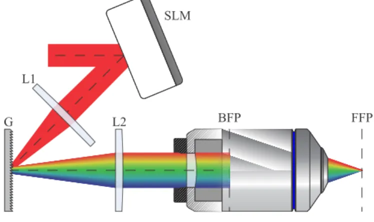
Here we calculate the two-photon axial response around the front focal plane of the objective for TF-CGH beams, as illustrated in the typical TF setup depicted in Fig. 1. Assuming a Gaussian spectral profile, the temporally focused pulse at the front focal plane of the objective can be described as a complex amplitude multiplied by a phase function:

E(x, y, ∆ω) = A(x, y) exp(−iα∆ωx − iβ ∆ω2₋∆ω2

2δ2) (1)

where A(x, y) is the complex amplitude function, α = 2π M

ω0g, ω0is the central frequency, ∆ω=

ω − ω0is the deviation from central frequency, M is the imaging system magnification, g is the

diffraction grating’s groove spacing, 2β is the applied GVD and 2√ln 2 δ is the full width half maximum (FWHM) of the spectrum of the pulse, assumed to be of a Gaussian shape. The first term in the phase function represents the diffraction off the grating. This result can be derived simply by imposing on the grating equation the condition that the first order of diffraction for the central wavelength is perpendicular to the grating (here we neglect the geometrical scaling of the x coordinate). Equation (1) can be used for numerical simulations of temporally focused pulse propagation with or without imposing the Fresnel approximation, as was done for the numerical simulations below as well as previously [6]. In the analytical derivation below we use the Fresnel approximation. Although not accurate for high-NA objectives [24], it captures the essence of the physical phenomenon. This assumption will be tested by comparing to both numerical and experimental results.

In order to model a CGH beam we describe the complex amplitude A(x, y) as a Gaussian envelope of width W multiplied by a speckle pattern, S(x, y):

A(x, y) = S(x, y)exp(−x

2_{+ y}2

2W2 ) (2)

and model the autocorrelation of the speckle pattern as a Gaussian of standard deviation σ : hS(ri)S?(rj)i = exp(−

(ri− rj)2

(5)

where ri= (xi, yi) and the brackets denotes ensemble average over different realizations of the

speckle pattern. We note that the exact functional form of the speckle pattern autocorrelation is determined mainly by the aperture of its Fourier transform [25]. However, the results pre-sented below are mostly affected by the autocorrelation width rather than by the details of the functional form. Furthermore, we assume that the speckle pattern is fully developed and thus obeys Gaussian statistics [25] so that moments of order higher than two can be separated into products of 2ndorder moments. This assumption is required for the analytical calculation of the two photon response.

FFP BFP SLM L1 L2 G

Fig. 1. Sketch of the TF-CGH setup. An Ultra-short pulse reflects off an SLM and is focused onto a diffraction grating (G) through a lens (L1). The first diffraction order is consequently imaged via a tube lens (L2) and an objective to the front focal plane (FFP) of the objective. The incident angle is such that the first order of diffraction is perpendicular to the grating. The SLM is imaged to the back focal plane (BFP) of the objective via lenses L1 and L2. Equation (1) describes the light distribution at the FFP of the objective.

We note that even though in general A(xi, yi)A?(xj, yj) is not a separable function, its

en-semble average is separable. Hence, we can solve separately for the x and y coordinates. The ensemble average of the two-photon signal at axial position z around the objective’s front focal plane is given by:

I2p(z) =

ZZ

h|E(r, z,t)|4idrdt =

ZZ

h|E(r, z = 0,t) ∗ h(r, z)|4idrdt (4) where E(r, z,t) is the electromagnetic field, h(r, z) =eik0z

iλ0zexp(

ik0

2zr2) is the convolution kernel in

the Fresnel approximation and k0is the wave number at the central wavelength λ0[26].

For simplicity, we first calculate for the x-coordinate. E(x, z,t) is given by the inverse Fourier transform to the temporal domain of Eq. (1) convolved with h(x, z) =qeik0z

iλ0zexp( ik0 2zx 2_{). Using} Eq. (2) we get: E(x, z,t) = FT_(∆ω→t)−1 {S(x)exp(− x 2 2W2− iα∆ωx − iβ ∆ω 2₋∆ω2 2δ2)} ∗ h(x, z) (5) = S(x) G(x,t) ∗ h(x, z) where: G(x,t) = (a + ib)−1₂ _exp(−(t−αx)2

2(a+ib) −

x2

2W2) , a =_δ12 , b= 2β

(6)

Using Eqs. (4) and (5) and separating 4th_{order moments into a product of 2}nd_{order moments,}

we can write the two-photon signal in the x-direction as:

(6) Ix2p(z) = Z h|E(x, z,t)|4idxdt = 2 ZZ dxdt[ ZZ dx1dx2hS(x1)S?(x2)iG(x1,t)G?(x2,t)h(x − x1, z)h?(x − x2, z)]2

Substituting Eq. (3) and denoting σxas the spatial autocorrelation width in the x direction,

we get the two-photon axial response for the x-direction: Ix2p(z) = Ax ((z − ∆z)2_{+ z}2 T F) 1 2 (7.a) ∆z= TR( σx/W)2TS (1 + T2 S + TR2) + (σx/W)2(TS2+ (1 + TR)2) zR (7.b) z2_{T F}=(1 + T 2 S+ TR)[2(1 + TS2)(σx/W)2+ (1 + TS2+ TR)(σx/W)4] [((1 + TR)2+ TS2)(σx/W)2+ 2(1 + TR+ TS2)]2 z2_R (7.c) where: TR=(W α) 2 a , TS= b a, zR= k0W2, Ax= π σxzR √ 2 a32 [(1 + T2 S+ TR2) + (σx/W)2(TS2+ (1 + TR)2)]− 1 2.

Here the TFS is manifested in the z-direction shift of the two-photon axial response denoted as ∆z. Solving for the y-coordinate we get similarly :

Iy2p(z) = Ay (2W2_z2 σy2 + z 2_{+ z}2 R) 1 2 (8) where Ay= pπ

2W zRand σyis the autocorrelation width in the y direction. The overall

two-photon axial response is given by:

I2p(z) = Ix2p(z) Iy2p(z) (9)

The parameters in our results have a straightforward physical interpretation. First, we note that in time domain, TF might be viewed as an ultra-fast line scanning. The parameter α = 2π_ωM

0g has units of

time

length and can be interpreted as the inverse of the ultra-fast line

scanning velocity. This can be seen from the expression for G(x,t) in Eq. (5). Next, two dimensionless parameters are defined in Eq. (7): TR=(W α)

2

a can be interpreted as the square

of the ratio between the ultra-fast line scanning duration and the pulse duration. TRgoverns the

two photon axial response of the TF pulse as is evident in Eq. (10.b) below. The GVD appears only in the dimensionless parameter TS=b_awhich is the ratio between the GVD and the square

of the pulse duration.

2.2. Limits of the results

In the case of smooth pattern (in the x-direction) such as a Gaussian beam (i.e. σx → ∞),

(7)

zT F→ 1+ T2 S + TR (1 + TR)2+ TS2 zR, ∆z → TSTR T_S2+ (1 + TR)2 zR (10.a)

The TFS, ∆z, for TS<< TR(which is typically the case) is proportional to the applied GVD,

in accordance with [9], with the proportionality constant given by the parameters of the experi-mental setup. We note that σydoes not directly effect the TFS. As σyincreases it merely reduces

Eq. (8) towards a two-photon axial response of a Gaussian beam in one lateral dimension. If, for a Gaussian beam, no GVD is applied (b → 0) Eq. (9) simplifies to:

I2p(z) ∝ 1 q z2_{+ z}2 R 1 r z2₊ z2R (1+TR)2 (10.b)

In this case, the result is a product of two terms. The first is the axial response of a 1D Gaussian beam with a Rayleigh range zR, this describes the non-temporally focused y-direction

axial response. The second is of similar form but with zRreduced by 1+ TR, this is the axial

confinement introduced by TF.

In the absence of TF (α → 0) Eq. (10.b) reduces to: I2p(z) ∝

1 z2_{+ z}2

R

(10.c) which is the two-photon axial response for a Gaussian beam with Rayleigh range zR. As is

evident from Eqs. (7) and (8), σx and σy play completely different roles in determining the

TFS, ∆z. While σx also controls ∆z directly through Eq. (7.b) the role of σy is indirect. It

attenuates the overall two-photon axial response as GVD is applied, thus practically limits the TFS.

∆𝑧

a

b

x

y

z

Fig. 2. a) Illustration of TF beam impinging on a grating when GVD is applied. The tem-poral shift between “blue” and “red” portions of the temtem-poral spectrum generates a spa-tial shift as the pulse scans the grating. This is equivalent to shifting the grating in the z-direction as long as the spectral portions can be considered as replicas of one another. b) The same effect but with TF-CGH beams. The autocorrelation width in the x-direction determines the lateral shift for which the spectral portions can be considered to be replicas of one another, which in turn determines the amount of TFS that can be achieved.

(8)

2.3. Physical interpretation

The physical interpretation of our results is illustrated in Fig. 2. We are particularly considering the following two aspects: a) equivalence of applying GVD to TFS and b) attenuation of the signal due to shifting between the spatial and temporal focus planes. We first discuss the equiv-alence of applying GVD to TFS and claim that it is related to the autocorrelation width in the x-direction. The effect of applying GVD on the temporally focused pulse can be understood as follows: Consider two different portions of the pulse spectrum, “red” and “blue”. These spec-tral portions are temporally shifted from one another due to the applied GVD. Each portion can be thought of as a (relatively long) pulse that scans the grating. Hence, at a specific temporal interval, the “red” and “blue” spectral portions are spatially shifted on the grating along the x-direction. This is equivalent to lateral shifting of different colors as they propagate after dis-persion off the grating. As a result, as long as the “red” and “blue” portions might be viewed as shifted replicas of one another, applying GVD is equivalent to shifting the grating in the axial direction, i.e. to shifting the temporal focus plane. Therefore, applying GVD is equivalent to TFS only if the autocorrelation width of the incident beam in the x-direction is large enough. This heuristic explanation is manifested in our analytical results by the dependence of the TFS on σx according to Eq. (7.b) and as is illustrated in Figs. 3 and 4. For a TF-CGH beam, this

means that applying GVD is equivalent to shifting the temporal focus only if the speckle size in the x-direction is large enough. Hence, passing the TF-CGH pattern through a spatial low-pass filter in the x-direction can be used to allow increased shift of the temporal focus.

The second aspect, attenuation of the signal with the TFS, depends mainly on the spatial fre-quency content of the TF beam. The temporal focused signal attenuates as it is shifted outside of the beam’s Rayleigh range. This corresponds to shift between the two axial profiles terms in Eq. (9). The higher the spatial frequency content of the beam, the shorter it’s Rayleigh range. Hence, beams with higher frequency content will cause faster attenuation of the signal as the temporal focus is shifted and vice versa. In the calculation above, the frequency content de-pends on the autocorrelation widths σxand σy. For TF-CGH beams this means that the signal

will decrease faster with TFS when the speckles are smaller. Therefore, passing the TF-CGH beam through a spatial low-pass filter (in both lateral directions) can be used to mitigate the attenuation of the signal with TFS. An alternative solution is to pass the beam through a spatial low-pass filter in the x-direction while shifting the spatial focus plane along with the temporal one by applying a quadratic spatial phase on the SLM.

Of the two effects described above the more significant one is the dependence of the TFS on σx. This is because decreasing both σxand σycause attenuation of the signal with applied

GVD, but only σxdetermines whether applying GVD is essentially equivalent to shifting the

temporal focus. This crucial role of σxis illustrated in Fig. 3. We note that since the peak of

the two-photon signal is generated at the TF plane, the TFS is given by the location of the axial profile peak. Figure 3(a) shows the axial profile of a TF Gaussian beam (σx→ ∞, σy→ ∞) as a

function of the applied GVD. In Figs. 3(b) and 3(c) either σyor σxare taken to be very small

correspondingly. As can be seen, decreasing σyattenuates the signal with the applied GVD thus

effectively mildly decreasing TFS. In contrast, decreasing σxeliminates the TFS altogether.

Finally, to illustrate in a clear manner the dependence of the TFS on the x-direction corre-lation σx, Fig. 4(a) shows the two-photon axial profile given by Eq. (9) as a function of σx,

with a GVD of 40000 f s2. The superimposed dashed line is the peak position for a TF Gaussian beam with the same amount of GVD applied and beam waist of σx. As can be seen, for large

values of σx the TFS is close to 20 µm. In stark contrast, for σx smaller than 3 µm the TFS

reduces, i.e. the axial profile peak shifts towards z= 0. Furthermore, the two-photon response attenuates rapidly as σxdecreases. In Fig. 4(b), each point shows the value of the TFS for which

(9)

z (µm) G VD (f s 2)

a

−20 0 20 40 60 0 2 4 6 8 10 x 104 z (µm) G VD (f s 2)

b

−20 0 20 40 60 0 2 4 6 8 10 x 104 z (µm) G VD (f s 2)

c

−20 0 20 40 60 0 2 4 6 8 10 x 104 0.2 0.4 0.6 0.8 1

Fig. 3. Axial profile as a function of the applied GVD for the case: a) σx, σy→ ∞. b)

σx→ ∞, σy= 0.3 µm. c) σy→ ∞, σx= 0.3 µm.

σ

x

( µ m )

z ( µ m )

a

2 4 6 8 10 −30 −20 −10 0 10 20 30 ₀ 0.2 0.4 0.6 0.8 1 0 5 10 15 0 5 10 15 20 σx( µ m ) ∆ z 1 2 ( µ m )

b

Fig. 4. a) Axial profile of a TF-CGH beam when applying GVD of 40000 f s2_{vs. σ} x(with

σy→ ∞). The superimposed dashed line is the peak position of a TF Gaussian beam with

the same amount of GVD applied and beam waist varying as σx. b) The TFS for which the

two-photon signal decreases to half its value with no GVD (denoted ∆z1/2), as a function of

σx. In both plots the minimum value of σxis 0.3 µm

value of the TFS is denoted as ∆z1_/2and is plotted as a function of σx. ∆z1_/2increases with σx and decreases towards zero as σxis decreased. In both Figs. 3 and 4 we used W = 10 µm as

the width of the Gaussian envelope described in Eq. (2) and a pulse duration of 170 fs, the other parameters were set as in the experiments described below. In Fig. 6 we present the ana-lytical results that are compared with the experimental and numerical ones. The comparison is discussed in the next section.

3. Numerical and experimental results

In order to verify the above analytical calculation we perform numerical simulations and exper-imental investigation. Below we describe both and compare to the analytical results.

The experimental setup is described in Fig. 5. The laser source used in the experiments is a Ti:Sapphire laser (MaiTai Deep-See, Spectra-Physics) producing pulses of 8 nm FWHM at a central wavelength of 800 nm. The pulses are passed through a grating compressor/stretcher in order to apply GVD. Next, the beam is magnified with a 10x beam expander and shined upon a phase-only SLM (LCOS-SLM, X10468-02, Hamamatsu Photonics), the resultant beam

(10)

FFP SLM L1 L2 G Ti:Sapphire Laser CCD Grating Compressor/Stretcher BE M M M xy Slits L3 M L G OBJ1 OBJ2

Fig. 5. Schematics of the experimental setup. Laser beam from a Ti:Sapphire laser is passed through a grating compressor/stretcher where GVD is applied. The beam then impinges on an SLM and focused into the TF setup, constituted of a diffraction grating, G, and an imaging system. L: Lens, M: Mirror, BE: Beam Expander, OBJ: Microscope Objectives, FFP: Front Focal Plane.

is Fourier transformed by focusing through a 100 cm lens. The phase imprinted on the SLM is predetermined using the Gerchberg-Saxton algorithm in order to generate a circle of 15 µm diameter. Control of the autocorrelation in x and y directions is achieved by passing the beam through a spatial low-pass filter, to which we refer below as low-passing. It is realized using a cylindrical telescope and a slit or, alternatively, an iris, that are set before the SLM. The slit used for x-direction low-passing (Fig. 6(b)) is a 1 mm slit located before the SLM. Since the SLM is imaged to the back aperture of the objective with 2x demagnification the effective low-passing is 0.5 mm of an overall objective back aperture of 5.4 mm. The y-direction low-low-passing (Fig. 6(c)) is performed similarly in the perpendicular direction. The iris used for low-passing in both x and y directions (Fig. 6(d)) is of 2.5 mm diameter which corresponds to 1.25 mm in the back aperture of the objective.

The TF setup is composed of a 300 lines/mm diffraction grating that is imaged with a 50 cm tube lens and a water immersion objective (Olympus, LUMPLFLN 60XW, 0.9NA). The front focal plane of the objective coincides with the TF plane when no GVD is applied. In the TF focal plane the beam excites a thin layer of Rhodamine 6G and the fluorescent light is imaged onto a CCD camera (CoolSNAP HQ2, Roper Scientific) through a second objective (Olympus UPLSAPO60XW, NA 1.0) and a tube lens.

In the numerical calculations we use Eq. (1) as our initial light distribution with the complex amplitude of a CGH pattern generated via the Gerchberg-Saxton algorithm. We then numerically calculate its propagation within the framework of vectorial theory [24], and calculate the two-photon signal.

Figures 6 and 7 summarize the comparison between the analytical, numerical and experimen-tal results. Figure 6 shows the analytical results with the same parameters as the experiments. The plots compare between the axial profiles without or with low-passing in either x,y or both x and y directions. Again, the difference in TFS between low-passing in the x and y direc-tions is immediately apparent when comparing Fig. 6(a) with Figs. 6(b) and 6(c) respectively. In Fig. 6(d) the iris size was chosen to produce speckles with approximately the same area as those produced by the slit. Despite the fact the speckles area is similar, low-passing in both directions results in less TFS than x-direction low-passing. This supports our theoretical results

(11)

−20 −15 −10 −50 0 5 10 15 20 0.1 0.2 0.3 0.4 0.5 0.6 0.7 0.8 0.9 1 z (µm) Nor m al iz ed si gn al a No GVD GVD 15000 fs2 GVD 30000 fs2 −20 −15 −10 −50 0 5 10 15 20 0.1 0.2 0.3 0.4 0.5 0.6 0.7 0.8 0.9 1 z (µm) Nor m al iz ed si gn al b No GVD GVD 15000 fs2 GVD 30000 fs2 −20 −15 −10 −50 0 5 10 15 20 0.1 0.2 0.3 0.4 0.5 0.6 0.7 0.8 0.9 1 z (µm) Nor m al iz ed si gn al c No GVD GVD 15000 fs2 GVD 30000 fs2 −20 −15 −10 −50 0 5 10 15 20 0.1 0.2 0.3 0.4 0.5 0.6 0.7 0.8 0.9 1 z (µm) Nor m al iz ed si gn al d No GVD GVD 15000 fs2 GVD 30000 fs2

Fig. 6. Each plot depicts the analytical results for the two-photon axial profiles for different values of the applied GVD. Plots a-d are for different slit widths corresponding to different spatial lowpass filters. a) No slit. b) 1 mm slit with its short axis in the x-direction. c) 1 mm slit with its short axis in the y-direction. d) 2.5 mm iris. The overlayed TF-CGH patterns are presented here for illustration, they are calculated for a single realization of a speckle pattern with a Gaussian envelope with the same parameters as the analytical calculation.

and heuristic explanation according to which low-passing in the x-direction controls the amount of TFS while in the y-direction it serves merely to mitigate the attenuation of the axial response with GVD. We also note that the axial response profile width increases for low-passing in the x-direction but not in the y-direction. This can be explained noting that the two-photon axial re-sponse, depicted in Eq. (9), is the product of x-direction and y-direction axial responses. Hence the narrower axial profile, which is the x-direction one, determines the width of the overall axial response.

Figure 7 shows the experimental and numerical plots corresponding to the plots in Fig. 6. There is a good agreement between the experimental and numerical results. Also, as is evident from comparing Figs. 6 and 7 there is a good agreement between the analytical and experi-mental results. We note that small discrepancies are to be expected due to assumptions taken throughout the calculation which are not completely accurate, such as the Fresnel approxima-tion and Gaussian statistics of the holographic pattern.

(12)

−20 −15 −10 −50 0 5 10 15 20 0.1 0.2 0.3 0.4 0.5 0.6 0.7 0.8 0.9 1 z (µm) Nor m al iz ed si gn al a No GVD GVD 15000 fs2 GVD 30000 fs2 −20 −15 −10 −50 0 5 10 15 20 0.1 0.2 0.3 0.4 0.5 0.6 0.7 0.8 0.9 1 z (µm) Nor m al iz ed si gn al b No GVD GVD 15000 fs2 GVD 30000 fs2 −20 −15 −10 −50 0 5 10 15 20 0.1 0.2 0.3 0.4 0.5 0.6 0.7 0.8 0.9 1 z (µm) Nor m al iz ed si gn al c No GVD GVD 15000 fs2 GVD 30000 fs2 −20 −15 −10 −50 0 5 10 15 20 0.1 0.2 0.3 0.4 0.5 0.6 0.7 0.8 0.9 1 z (µm) Nor m al iz ed si gn al d No GVD GVD 15000 fs2 GVD 30000 fs2

Fig. 7. The experimental and numerical results corresponding to the ones presented in Fig. 6. Each plot depicts comparison between experimental (circles) and numerical (solid line) results. The overlayed images are the corresponding experimental TF-CGH patterns.

4. Conclusions

We have investigated the effect of applying GVD on TF-CGH beams theoretically and exper-imentally. We have shown that the equivalence between applying GVD and generating TFS depends mainly on the autocorrelation width of the CGH pattern in the x-direction, which is the direction in which the ultrashort pulse diffracts off the grating in the TF setup. Correspond-ingly, low-passing in the x-direction was shown to increase the TFS, in contrast to low-passing in the perpendicular direction. Therefore, temporally focused excitation can be axially shifted by dispersion only when the autocorrelation width of the illumination in the x-direction is sufficiently large. Signal attenuation with applied GVD was shown to be dependent on the au-tocorrelation in both lateral directions, due to the shift between the temporal and spatial focal planes. Although low-passing in both lateral dimensions can serve to increase the TFS, it also increases the speckle size which may not be desirable for some applications such as multi-photon optogenetics. The investigated effect, in which the two-multi-photon excitation is controlled in 3D by manipulating both temporal and spatial frequencies of the incident light, can be useful for optogenetics, nonlinear microscopy and micro-machining.

(13)

Acknowledgments

DO acknowledges financial support by the European Research Council starting investigator grant SINSLIM 258221, by the I-CORE Program of the Planning and Budgeting Commit-tee and the Israel Science Foundation and from the Laboratoire Européen Associé NaBi be-tween the CNRS and the Weizmann Institute. VE acknowledges financial support by the Hu-man Frontier Science Program (RGP0013/2010), the ‘Fondation pour la Recherche Mèdicale’ (FRM Èquipe) and the ‘Agence Nationale de la Recherche’ (grants ANR-12-BSV5-0011-01, Neurholog) and by the France-BioImaging infrastructure supported by the French National Re-search Agency (ANR-10-INSB-04, Investments for the future). OH acknowledges the program Nanotechnologies France-Israël for financial support.