Multispektrale Fotoaufnahme für die Detektion von Hautkrebs

(1)

Systems Ingineering

Infotronics

Thesis 2014

Michael Schmid

Multispectral photograph for the

detection of skin cancer

Expert Martial Geiser

(2)

(3)

INDEX

1 PREFACE ... 1

2 INTRODUCTION ... 1

2.1 What is the problem ... 1

2.2 Similar projects ... 1

2.3 Our solution ... 2

2.3.1 Melanin detection ... 2

2.3.2 Blood analysis (hemoglobin detection) ... 3

2.3.3 Deep view ... 3

3 SPECIFICATIONS ... 4

4 HARDWARE ... 4

4.1 Image acquisition - Camera ... 4

4.2 ... 5 4.2 Optpical setup ... 6 4.3 Illumination ... 7 4.3.1 LED ring ... 7 4.4 Casing ... 8 4.4.1 Reference regions ... 8 5 SOFTWARE ... 9 5.1 Image acquisition ... 9 5.1.1 Main window ... 9 5.1.2 Analysis window ... 10 5.1.3 Settings window ... 11 5.2 Analysis ... 12 5.2.1 Optimisation ... 12 5.2.2 Measurement ... 17 6 FUTURE EXTENSIONS ... 21 6.1 Optical system ... 21 6.2 Image acquisition ... 21 6.3 Data storage ... 21 6.4 Analysis ... 21 6.5 Casing ... 21 7 CONCLUSION ... 22 8 SOURCES ... 22 8.1 Literature ... 22 8.2 Figures... 22

9 DATE & SIGNATURE ... 22

10 APPENDIX ... 23

(4)

10.1.1 LED controller ... 23 10.1.2 LED ring ... 31 10.1.3 Parts list ... 35 10.2 Software - general ... 36 10.2.1 Class diagram ... 36 10.2.2 MainTimer ... 37 10.3 Software - code ... 38

10.3.1 IdsSimpleLiveDlg (main window) ... 38

10.3.2 Analysis ... 44

10.4 Tests ... 53

10.4.1 Melanin and hemoglobin tests ... 53

10.4.2 Prove of melanin detection ... 54

10.5 Future extensions ... 56 10.5.1 Image acquisition ... 56 10.5.2 Data storage ... 57 10.5.3 Analysis ... 57 10.5.4 Developement tips ... 59 10.5.5 Contact informations ... 59

(5)

1 PREFACE

The results of this project aren't just my earnings. Therefore I first want to thank everyone who helped me with patience and competence. A special thanks to my expert Martial Geiser, who particularly supported me with my work. He was always there to answer questions, and to acquire solutions together. A thanks to Frederic Truffer and Helene Strese, they gladly answered questions, and gave me convenient tips. I also want to thank Olivier Walpen and Serge Amoos for helping me with electronics and casing. Finally an acknowledgement to Dr. Gianadda Elisabeth, who supported us with valuable ideas and standards.

This project was a great experience doing a step in the direction of the real working world. Finding different solutions, deciding for one, and then handling the ramifications was an exiting experience, which can't be taught in regular class. Due to the vast scope of this project, it was really interesting to participate the different domains of biology, optics, hardware and software development, and combine them to one extensive project.

2 INTRODUCTION

2.1 What is the problem

Since skin cancer is the most common kind of cancer in Switzerland, its detection and treatment consumes a high amount of time and money. Due to subjective diagnosis by eye, based on experience of the dermatologist, a surgical operation will take place - or not. Here the product can show his strengths. Substantiate the decision of the dermatologist, or maybe indicate another view. It will be possible to avoid unnecessary surgery, sparing a lot of trouble. A meeting with Dr. Gianadda helped to understand the problem, and led the project into the right direction. We got a view on the FotoFinder, which will be described on the next chapter.

2.2 Similar projects

A commonly used system is the FotoFinder. It is a highly developed device with a broad spectrum of sophisticated functionalities. The aviable full body scan, and the vast database are just two of its strengths. The body scan will indicate critical points, wich then can be scanned with the additional fullHD camera. Of course those measurements have an outstanding quality, yet it just provides one RGB image with the entire light spectrum.

(6)

Here comes the opportunity of our device, which provides a multispectral imaging. This multispectral imaging not only shows the surface, but also allows a deeper view itno the skin. A melanin analysis, and also a oxy/deoxy - hemoglobine determination is possible with those capabilities.

This project is based on a previous solution, which was developed with a similar specification and the same purpose. The initial goal was to make the device smaller, and to develop further software. Yet the result is a completely independent solution. [1]

2.3 Our solution

The main method lies in the melanin, but also in the hemoglobin detection. It can be achieved by illumination with particular light spectrums. The camera measures the amount of reflected/scattered light, which can give indications to a possible risk.

2.3.1 Melanin detection

The melanin detection becomes possible through the known absorption behaviour of the entire light spectrum. Specific wavelengths can be measured, and then compared to the original absorption function. Following graph shows the chosen wavelengths for the measurement. A point below 390nm can't be implemented because of the sensivity of the camera. Nevertheless, the avaiable wavelengths are perfectly adequate.

390nm

470nm

520nm

610nm

(7)

2.3.2 Blood analysis (hemoglobin detection)

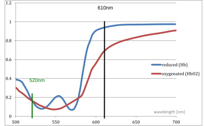
The blood analysis uses a procedure quiet similar to the melanin detection. The known graph of oxy and deoxy-hemoglobin transmission is essential. A smart choice of two specific wavelengths already enables the possibility to distinguish oxygene rich, and oxygene poor hemoglobin. One point is set where the sensivitys are very close, the other point stands for a maximal difference. The ratio of these two values then indicates the amount of oxy and deoxy-hemoglobin.

Figure 3: hemoglobin transmission

2.3.3 Deep view

Beside the methods shown, the remarkable feature of looking into the different layers of the skin is definetly worth to mention. Especially the infrared LED with 880nm wavelength enables a really deep view beyond the epidermis. This should allow locating aberrations even deep under the skin. Following measurement shows the speciality of every LED. Note the vein, which was found in deeper regions.

Figure 4: Measurement example

0 0.2 0.4 0.6 0.8 1 1.2 500 550 600 650 700 reduced (Hb) oxygenated (HbO2) wavelength [nm] se n siv ity / tra n sm is sion 520nm 610nm

(8)

3 SPECIFICATIONS

This project attends to the task of taking a multispectral image acquisition of a specific skin region, with a diameter of 1 Inch (about 25mm). The five images will pass trough an analysis algorithm, which confirms or disproves the suspicion of skin cancer. The product should provide following functions:

Calibration: The device has two calibration functions. One essential main calibration with a reference, but also a small gauging with each measurement.

Image acquirement: A measurement should be very simple. A button on the camera will provide maximal usability. Also the procces should not take longer than a second.

Display: After the measurement a brief overview of the taken images will be shown. Which images exactly, (raw data / analyzed data / combo) will be determined in a later instance.

Analysis: The software provides an evaluation with following criteria: - Determination of melanin amount.

- The ratio of Oxy- and Deoxyhemoglobine. - Analysis of contours.

Database: Every measurement will be stored properly.

Properties: The software contains different setting possibilities. (such as contrast, exposure time ect.)

4 HARDWARE

4.1 Image acquisition - Camera

The recent semester project intensively approached the choice of the right camera. The decision fell to the UI-1222E from the german company "uEye". It is a CMOS camera, also aviable with mono technology. This is a big advantage for our purposes, due to its improved dynamic range. The goal was to go with the newest and best aviable technology. The reward was a professional camera with outstanding characteristics and very good documentation, which allowed determined and effective developement. Following table shows the most important technical specifications. For more details and a very detailed documentation explore the CD.

(9)

The relative sensor sensivity is definitely worth a special mentioning. This camera can see widely beyond the human eye, or other similar cameras. It allows the usage of a 880nm LED. The detailed graph is shown below.

4.2

Figure 6: Camera specifications

(10)

Optpical setup

4.2.1.1 Lense setup

The first prototype in the semester project [2] showed that a single lens can't achieve the desired quality demands. Therefore a system with two lenses was calculated, and implementated. This time an achromatic lens was used, due to the error correction of different wavelengths. Following two lenses were used:

 AC 050 - 010 - B

 Bi. +; 50/12,7 gef.

The distance between object and first lens is 83mm, the distance sensor <-> second lense amounts to 2mm. Yet it can't be measured properly, since the montage doesn't allow it. The same for the distance between the two lenses, which is around 10mm. Nevertheless those values are not important, since a new optical system would require a new calculation anyway.

The assembly of the optical system was a challenging task, because a small variation in the distance between the optical elements already affects the image quality. The laser cutting machine was used to create the required parts. The plans are aviable on the CD. HINT! The lenses are clamped with screws, which should hold fine. Still, I recommend a careful usage. Never shake the device! A very small shift of a lense could already have impact on the image quality.

4.2.1.2 Pinhole

Already in the semester project we had too much light on the sensor. This problem was solved by a pinhole, which also improved the image quality. Different versions between 0.5mm and 2mm were tried, while the 2mm had the best acuity. The pinhole is directly attached to the inner side of the second, big lense.

(11)

4.3 Illumination

4.3.1 LED ring

The key to a good measurement is the proper lighting of the object. The assembly of the LED's plays a crucial role to a homogenous picture. After some tests it has been shown that a specific angle of the LED's is not absolutely required. This enables the possibility to design the LED ring with a simple PCB. Still, the assembly has to be a perfectc circle. It led to some major problems with PCAD (software for PCB design) since it is not intended to work with round objects. Nevertheless the board was created. It is shown in the picture below. For schematic, PCB layout, calculations and partlist see appendix_10.1.2.LED

controller

The camera provides a very useful feature with its given inputs/outputs. Unfortunately it hasn't enough outputs to actuate every LED separately. Therefore a simple solution with a PIC was found. The trigger button is connected with the camerea as well as the PIC. Now the start signal will launch both parallel. The PIC is programmed to power on each LED group for 200ms. This gives the camera enough time to take the picture. The PIC was implemented on a seperate PCB, which can be easily connected with the LED-Ring, as shown in the following picture. For schematic, PCB layout, partlist and details about the PIC programming see appendix_10.1. The Led ring and the PIC controller share the same partlist.

Figure 9: LED ring PCB

(12)

4.4 Casing

The casing was realised with the 3D printer. Serge Amoos created the plans in Autodesk Inventor. They are avilable on the CD. Following picture shows a view of the 3D model.

4.4.1 Reference regions

The white regions are crucial for the gain adjustment of each measurement. This part is basically made out of a simple ring, created with the laser cutting machine (plans on CD). Two stripes of thick paper are glued to this ring. They have a width of 10mm. It is very important to keep the ring on the right angle during the masurement.

HINT! The raw data will include the reference regions. A black rectangle indicates the region used for the adjustment. Make sure that the entire rectangle only contains the designated white region.

Figure 11: 3D model of casing

Figure 12: Calibration region

(13)

5 SOFTWARE

5.1 Image acquisition

5.1.1 Main window

The data acquisition should be as simple as possible. Pushing the button will trigger the camera and the Illumination. A user-friendly and simple GUI will help to take pictures and make an analysis with a minimum effort. Following picture shows the user interface that will appear when the user opens the program. It provides a big display window for a live video stream, an optimal preview for measurements. The window provides following options:

 Next: Make a quick measurement, without the need of opening the analysis window. It will make the analysis automatically and save the results. When the "Show quick Result" checkbox is open, it will display the result of the melanin and blood analysis.

 Analyze: This button will open the Analysis window for further options.

 Patient Informations: Please enter the patient information here.

 Calibration Mode: This enables the calibration mode. In this mode an absolutely homogenous and white surface is needed. The images will be saved into images/Calibration, where they can be used as reference for a proper calibration.

 Settings: Open the settings for exposure time adjustment, or loading parameters.

 Exit: Close the program.

(14)

5.1.2 Analysis window

This window allows custom options for the measurement. An example body represents the patient, where the location of the measurement can be indicated. The patient informations will be taken automatically from the main window.

The window provides following options:

 Homogenity Adjustment: Since the homogenity adjustment is the most time consuming procedure, it is hereby available to perform voluntary. After the adjustment the results will be shown. They can all be closed at once with the "Close" button near the initial button.

 Melanin Analysis: This button will do the melanin analysis, and show the results. Also these images can all be closed at once with the nearby "Close" button.

 Blood Analysis: Same procedure for the oxy/deoxy-hemoglobine determination.

 Show / Close Images: This button will show or close all taken pictures.

(15)

5.1.3 Settings window

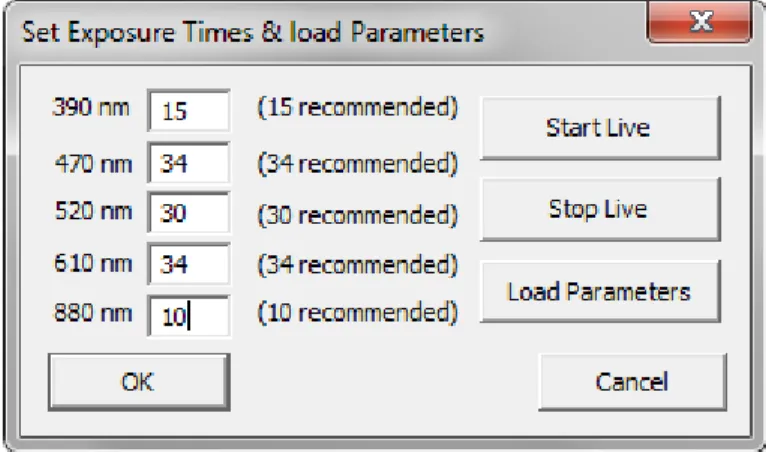
This window is supposed to perform desired changes to the exposure times. Try not to vary too much from the recommended values since they are well balanced. Of corse the gain adaption will always correct the difference, still it would bring unwanted noise into the system. The exposure times will be saved in settings.txt in the Parameters folder. With the "Load Parameters" button, it is possible to load earlyer saved camera parameters from the Software "uEye Cockpit". It is recommended to stop the livestream for that. Note that this option hardly was investigated because it wasn't needed at all. There may be further adjustements needed to properly load given parameters.

(16)

5.2 Analysis

Since important operations are pretty much implemented with fitting methods, almost every capture will be closely linked to an actual function. If so, the name of the method will be mentioned right under the title.

5.2.1 Optimisation

Before an actual measurement can take place, the images need to be optimized. Even with good balanced exposure times and proper illumination, there are slight differences between the images, which would decrease the accuracy of the measurement. The optimisation takes place in two steps. First the gain will be adjusted, to put all images on the same level. Secondly the homogenity will be evened. The exact procedure is explained in this chapter. An overview is shown in the following exaggerated picture, to emphasize the process.

5.2.1.1 Set gain of an image

Software solution in appendix_10.3.2.2

This Method has a really simple task. It takes an image (Mat), adjust its gain, and then returns the newly calculated image. There are two parameters available (alpha, beta). Following formula shows how they work:

g ai n ho m o g en it y

(17)

The function will recalculate every single pixel with this formula. Alpha is the gain factor, while beta works as offset.

5.2.1.2 Even out the images with gain adaption Software solution in appendix_10.3.2.3

The goal of this method is to ajust the gain of all images to a common level. Each image has two white calibration regions on its right and its left. The average value of this regions will be calculated. Usually these values should be quiet similar. If they vary by an increased amount, there are two possibilities of irregular lighting. Either a LED is not working or illuminating weak, or there is an external lightsource disturbing the lighting. It could also be that the calibration papers are not attached propperly or with a different angle, the rectangles will hit a part of skin instead of paper. A warning message will show if one of these problems occurs. If everything runs right the mean of these two avarage values will provide the proper gain adjustment.

The intended gain can now be easily calculated by following formula:

Now a call of the setGain() Method will do the actual gain adjustment. The value was carefully chosen to bring the white calibration region of each image into saturation (max value = 255).

(18)

5.2.1.3 Homogenity issue

One of the most important requirements for a proper measurement is a good homogenity of the image. It is almost only influencted by the lighting. Since the solution for the illumination already attempts to achieve an optimal result, there must be an additional software support for an optimized homogenity of the picture. This will be achieved with the help of a calibration. Threfore an image of a clean white surface will work as a reference. From this reference a pattern will be created which can be utilized to even out further measurements.

The actual procedure works like a compressor (in audio domain). There will be a certain treshold, in this case the mean (average) value of the picture. So every value that lies above the treshold, will be attenuated. Every value below it, will be increased. In the end the dynamic range will be much smaller, the values are closer to each other, which means the picture has a better homogenity.

Figure 18: overview of homogenity adjustment

(19)

5.2.1.4 Create the stamps

The name of this method was chosen, because it creates a file comparable to a stamp. The stamp then can be used on an image, to alter its appearance (in this case homogenity). So the goal is having a specific correction-factor for each single pixel. The created textfile will contain all this information.

First the calibrationImage will be loaded. They are stored in /images/Calibration. Then the average value of all picture will be calculated individually, and stored in the mean[] Array. (Don't confuse it with the mean for melanin detection, which is a mean of all the images together)

∑

Now a loop will go through the entire image, calculating the correction factor for each pixel with following formula:

Because of the fraction, the correction now is a value around 1 with several decimal places, which results in a double. Considering that the images just have a Byte per pixel, the output can't be another image. Since there is the need of a permanent accessibility of this data, there has to be another way to store it. Unfortunately the installed Visual Studio does not support many database possibilities. Therefore the data is stored in stamp-textfiles, which will be created in the /Parameters folder.

Please note the need of an absolute exact and unambiguous format of the textfiles. Already the slightest change can result in absolute unreadability. Like the following little example shows, the values are just seperated with a space " ".

(20)

5.2.1.5 Adjust the homogenity

Now that the stamps are ready to use, this method finally takes an image, uses the stamp(correction) on it, and returns a proper homogenity-adjusted result. It again loops through all the pixels, and makes a division of the pixelValue by the correction.

There is a chance that the adjusted value can hit a higher value than the maximal allowed ( > 255). This would result in a glitch, where the value becomes zero (black). To avoid this problem, a factor and offset was added. With a suggested factor of 0.8 the function won't hit any saturation.

HINT! If the image shows randomly spread black dots, try to use a factor < 1, and/or a negative offset, to not hit saturation!

Since the adjustment is really time consuming, the parameter "i" allows to take a specific image.

Following picture shows a successful homogenity adjustment on a test image.

Figure 21: Flowchart of homogenity adjustment

(21)

5.2.2 Measurement

In this chapter we will see the actual analysis of the measurement. These functions will implement the investigation of signs for skin-cancer. There are three important symptoms, which will be the focus of this Project:

 high amount of Melanin

 anomaly of oxy-and deoxy-hemoglobin

 irregular shapes of birthmark

Again, every of these procedures is implemented with a fitting method. 5.2.2.1 Melanin analysis

One of the most important symptoms, a highly increased amount of melanin. The most obvious sign of a mutation of melanocytes. Now the first and most important task is the detection of the melanin in the first place. The chosen solution is to compare the taken pictures with the known light absorption graph of melanin (see 2.3.1). For better access, the Graph was imported to excel with help of WebPlotDigitizer [3]. Since it makes more sense to work with the permeability instead of the absorption, a transformation with following formula took place:

The transformation itself would result in a value between zero and one. So the factor of 255 is used to stretch the value over the available range of a Byte. Also the values below 380nm were removed, since the lowest available wavelength is 390nm. The camera probably would not be able to get any lower. Following picture shows the before-after Graph.

Now the interesting part about the import into Excel is the possibility to create an approached trendline polynomial function. Already a function with 4th order turned out to be quiet accurate. So here is the final function:

y = -2.0126E-08x4_{+ 4.6262E-05x}3_{- 3.9755E-02x}2_{+ 1.5632E+01x - 2.2747E+03}

Figure 23: Melanin absorption to permeability transformation

wavelength [nm] ab so rpt io n pe rm eab ili ty

(22)

For easy use, there is a method implemented which will return the permeability value in function of the wavelength: double melaninFunction(double wavelength)

Now we have everything to get the factor between the desired curve, and the actual measured image. The factor can be calculated with following formula:

The value of the factor will roughly vary between 0 and 2, where 1 means that the measured and the intended melanin value are identical. Now for a better visual overview, the function above will be extended, and now saved in an image instead of an array.

Assuming a 100% match, the entire factorImage would be grey-> 128. If it goes more in direction of white, (128+) it means that the measured value is higher than the melanin value. If it goes in direction of black (128-), the measurement is lower than the melanin value. Of corse this will count for every pixel, and result in an image.

Now the five images will be merged to only one image, to gain some better overview. Following function calculates the mean (average) of all images, and saves it to a single new image.

∑

Last but not least, there has to be a little calibration to adapt the values to real world environment. This is achieved with the calibration factor melaninIndex. This index is based on a dark skin sample.

And there we have a result! The brighter the Image, the more melanin was detected. Beside the mean of the melanin, there is another result image available. It represents the standard deviation. Every pixel will be calculated with following formula:

√ ∑

lower _match! higher

0 128 255

Figure 25: Dial for the factorImage

Figure 24:example of melaninMean

(23)

5.2.2.2 Prove of melanin detection

This chapter will prove that the analysis detects actual melanin. Of course there will be always other factors that can influence the measurement, but following tests should show that it really focuses on melanin. Please consider that the last image (610nm) is not very much affected by melanin, so its value is rather negligible. The excel files with the calculations and graphs can be found on the CD. For more details about the tests see

appendix_10.4.2.

Following graph shows a summary of the important measurements. It is clearly visible that the two "tricked" examples are way off, where the actual skin scan shows a surprisingly high accuracy.

5.2.2.3 The evaluation

After the validating tests we can assure that the measured graph represents pretty much the melanin permeability. But since it is a relative value, how do we determine the effective amount of melanin? For this procedure a calibration with help of the calibrationFactor is necessary. Following graph shows just two measurements - a brown and a white skin.

0.00 50.00 100.00 150.00 200.00 250.00 300.00 350.00 300 350 400 450 500 550 600 650 700 750 melanin permeability brown paper black plastic skin

Figure 26: Measurement of different surfaces

wavelength [nm] p erm eab ili ty

(24)

The very simple solution is to chose a calibrationFactor setting, so that the darkest skin example exactly matches the melanin permeability curve. It now represents the reference. Now every measurement with less melanin will be above this value. Since it is a dark skin color, it is unlikely that a regular measurement will go much deeper than this value. If the value has a distinct low value, it can be considered as potential hazard. To simplify the result, a average value of the 4 wavelengths is sufficient. This procedure will be done for every single pixel, and finally be accessible in the melaninMean result image.

5.2.2.4 Blood analysis

Software solution in appendix_10.5.3.1

Since the focus of the project was on the melanin detection, the blood analysis is held very simple. One single operation will take the 520nm, and the 610nm image for a ratio calculation (see 2.3.2). Following formula is used:

The factor of 128 has the same purpose like the melanin measurement before, it displays a value between roughly 0 and 2 with grayscales. For proper use there is a need of some tests and a calibration, which is not implemented yet.

0.00 50.00 100.00 150.00 200.00 250.00 300.00 300 350 400 450 500 550 600 650 700 750 Melanin permeability Brown skin white Skin avg. white Skin

avg. brown Skin

Figure 27: Evaluation of melanin measurement

wavelength [nm] pe rm ea bi lit y

(25)

6 FUTURE EXTENSIONS

Unfortunately the scope of this project often exceeded the available timeframe. Therefore compromises had to been made. Since this project will be continued, this chapter will mention a few points worth of improvement.

6.1 Optical system

The lenses are assembled in a construction rather determined for test purposes. Surely it absolutely accomplishes its task, yet the system could be smaller. Also most of the weight of the device comes from the optical system. The camera has additional connection possibilities to support a much smaller system. I would highly recommend a new customised optical system.

6.2 Image acquisition

The camera currently needs 200ms per image. However, if a faster acquisition is needed, there would be the possibility to use the camera intern buffer. Also a I2C communication between PIC and camera processor would optimize the duration of the illumination. For details see appendix_9.5.1.

6.3 Data storage

The current project creates a folder for each patient, and saves the measurements with the actual date and time. A more professional solution would be a SQL database, which would allow a wide range of customisation. Also online access for further analyses, processing or just data exchange would be possible. For an already worked out concept see appendix_9.5.2.

6.4 Analysis

Fortunately the melanin analysis could be finished with great results. Yet the hemoglobin and conture methods are just prototypes. They definitely need some further development. This is probably the most important task to begin with. Still, with some tests and a proper calibration, the hemoglobyne procedure already may yield some usable results.

6.5 Casing

Unfortunately the time run out to improve the casing. An increased diameter of the tube would allow a larger usable image. Also the height should be slightly increased for a better montage. An additional fixture of the reference regions would prevent them from shifting. Nevertheless I would recommend a revised optical system, which would imply an entire new casing.

(26)

7 CONCLUSION

The choice of the camera turned out to be rewarding, and also the range of wavelengths brought good results. The setup was changed to 390nm, 470nm, 520nm, 610nm and 880nm, where especially the infrared LED enables some interesting opportunities. The final results are very persuasive, a melanin determination with such high accuracy is a solid cornerstone for this device. I see great potential for the future, where targeted development for optimized oxy and deoxy - hemoglobin determination will complement the device to a great product. The outline analysis may be redundant, since the FotoFinder already includes this feature. A redesign of the optical system will allow a much lighter and smaller case, allowing it to be competitive to other products.

8 SOURCES

8.1 Literature

[1] Documentation of previous project, available on CD in illustrations folder [2] Semester Project available on CD in illustrations folder

[3] WebPlotDigitizer: Program for graph transcription http://arohatgi.info/WebPlotDigitizer/

8.2 Figures

Figure 1: http://www.fotofinder.de

Figure 2: http://www.cl.cam.ac.uk/~jgd1000/melanin.html

Figure 3: http://biomedicaloptics.spiedigitallibrary.org/article.aspx?articleid=1102785 Figure 6: uEye Documentation

Figure 7: uEye Documentation Figure 8: Simulation

Figure 16: Photoshop

Figure 19: http://www.youtube.com/watch?v=91qs3fux5HY -> Audio Compressor explained

9 DATE & SIGNATURE

(27)

10 APPENDIX

10.1 Hardware

10.1.1 LED controller

10.1.1.1 PIC Programming

10.1.1.1.1 Timer

For further easy to use timing, a timer with a 10ms elapse will be implemented. To achieve this interval, a Timer0 Value of 0x63BF is used. With this timer every exposuretime can be achieved with a factor of 10ms.

10.1.1.1.2 Interrupts

Following picture helps configuring the Interrupt Registers. GIEH = 1 for global Interrupt enabling.

We use the first Pin for interrupts, so INT0, INT0IE has to be 1.

(28)

10.1.1.1.3 Inputs / Outputs

Following Picture helps configure the ANSELx Registers. For geting outputs, ANSELA, will be entirely 0's.

(29)

10.1.1.1.4 Code

10.1.1.1.4.1 User.c

This method is basically used to initialize the PIC. IT defines Inputs/Outputs with TRISx and ANSELx, configures the timer with T0CON, and sets the timer elapsing time with TMR0H and TMR0L. Also the Interrupts will be enabled and configured with GIEH/PEIE/INT0IE/INTEDG0. With LATA = 0x00 we make sure that all leds are disabled at the beginning.

HINT! Use LATA to define all outputs/inputs at once everytime, instead of PORTA.RAx. Yes you have to reasign all outputs everytime instead of just one, but you will avoid some unwanted behaviour.

void InitApp(void) { //Port Declarations TRISA = 0b00000000; ANSELA = 0b00000000; TRISB = 0b11000001; ANSELB = 0b00000000; // Timer 0 T0CON = 0b00001000; TMR0H = 0x63; TMR0L = 0xBF; // 0x63BF = 10ms //Interrupts GIEH = 1; PEIE = 1;

INT0IE = 1; // Enables the INT0 external interrupt INTEDG0 = 1; // Set to interrupt on rising edge // Timers & Interupts

TMR0IE = 1; // Enables the TMR0 overflow interrupt TMR0IP = 1; // Timer0 -> High priority

LATA = 0x00; start = false; counter = 0; }

10.1.1.1.4.2 System.c

This method is used to set the oscillator frequency. It is common use to just let the oscillator run on his maximal frequency, which in this case is 16 MHz (0b11110010).

void ConfigureOscillator(void) {

OSCCON = 0b11110010;

while(!HFIOFS)

{

// do nothing until Oscillator is stable }

}

10.1.1.1.4.3 Interrupts.c

This method is essential for the work with timers. Everytime the timer elapses, it will call the interrupt sub routine. This will restart the timer, and also increment the counter wich then can be used to determine the illumination time.

void interrupt high_isr(void) {

if (INT0IF) {

(30)

TMR0ON = true; //Enable Timer0 start = true;

INT0IF = false; //clear flag }

if (TMR0IF) {

TMR0H = 0x63; TMR0L = 0xBF;

TMR0IF = false; //clear flag counter++;

} }

10.1.1.1.4.4 main.c

This method will actually set the LED states to on or off. Depending on the value of the counter, it will chose the fitting LED. Unfortunately the case parameters have to be static. They are basically x*lightTime + offset. So if a change of the illumination time is desired, every case has to be updated separately. The offset parameter is there to help synchronize the camera and the PIC. It is possible to play around with the offset to get better results. -5 is a good value for an illumination time of 200ms. After 1150ms the cycle is over, and everything will be resetted to be ready for the next measurement.

/******************************************************************************/ /* User Global Variable Declaration */ /******************************************************************************/

static int lightTime = 20; // factor 10ms!

static int offset = -5; // offset for camera synchronisation

/******************************************************************************/ /* Main Program */ /******************************************************************************/

void main(void) {

// init values

ConfigureOscillator(); InitApp();

LATA = 0x04; // let green LED on as default //LATA = 0x00; // set all LEDS off

while(1) { if(start) { switch(counter) { // lightTime + offset case(15): LATA = 0x01; break; // 2*lightTime + offset case(35): LATA = 0x02; break; // 3*lightTime + offset case(55): LATA = 0x04; break; // 4*lightTime + offset case(75):

(31)

LATA = 0x08; break; // 5*lightTime + offset case(95): LATA = 0x10; break; // 6*lightTime + offset case(115):

//LATA = 0x00; // turn all LED's off LATA = 0x04; // turn green LED's on TMR0ON = false; // stop timer

start = false; // reset start flag counter = 0; // reset counter break; } } } } 10.1.1.2 Schematic

Following page will show the entire schematic of the LED Controller. The core of this PCB clearly is the PIC18 who is controlling the entire illumination process. Since the PIC would not have enough output power, he triggers five MOSFETS, which will then supply the actual LED's. Each of this MOSFETS has two dedicated resistors to enhance their performance:

The connectors are from left to right: connection to LEDs, connection to camera, and programming interface.

C1 and R11 are part of the basic circuit needed for the PIC18, while R12 is a Pull-up resistor for the button.

(32)

(33)

10.1.1.3 Layout

The next page will contain detailed information about the Top and Bottom layer, and also a version with placed components. Following picture shows a overview of all the layers combined.

(34)

(35)

10.1.2 LED ring

10.1.2.1 Schematic

Following page will show the entire LED ring schematic. Each domain consists 4 parallel LED's with their pre-resistors. The calculation of the resistors is shown in following Table.

Vcc = 5V

R = (Vcc-UDx)/I

LED1: 390nm

UD1 =3.2V

ID1 = 20mA

RV1 = 90Ω

Appropriate resistor:

91Ω

LED1: 470nm

UD1 =3.7V

(3.4V typ.)

ID1 = 20mA

RV1 = 65Ω

Appropriate resistor:

68Ω

LED1: 520nm

ID1 = 20mA

UD1 = 3.2V

RV1 = 90Ω

Appropriate resistor:

91Ω

LED1: 610nm

ID1 =20mA

UD1 = 2V

RV1 = 150Ω

Appropriate resistor:

150Ω

LED1: 880nm

ID1 = 20mA

UD1 = 1.32V

RV1 = 184Ω

Appropriate resistor:

180Ω

(36)

(37)

10.1.2.2 Layout

The next page will contain detailed information about the Top and Bottom layer, and also a version with placed components. Following picture shows a overview of all the layers combined.

(38)

(39)

10.1.3 Parts list

Following Table contains the Part List of both components, the LED ring and the LED Controller. LED's

Quantity Description Value Art-Nr. vendor Price

4 SMD LED 390nm 1890331 Farnell SFr. 12.15 4 SMD LED 470nm 8529965RL Farnell SFr. 3.67 4 SMD LED 520nm 1716766RL Farnell SFr. 0.42 4 SMD LED 610nm 8530009 Farnell SFr. 0.30 4 3mm LED 880nm L-7104SF4BT Distrelec SFr. 0.81 Resistors

4 pre - resistor for 390nm 91Ω STOCK

7 resistor for PIC/MOSFET 10kΩ STOCK

5 resistor for MOSFET 51Ω STOCK

Capacitors

2 decoupling 100nF STOCK

Transistors

5 Mosfet: supply for LED's MMBF170 STOCK

PIC

1 PIC18(L)F2X/4XK22 PIC18F2XK22-/SO STOCK

Connectors

1 straight 6 Pins STOCK

1 90° angle 6 Pins STOCK

(40)

10.2 Software - general

This chapter will cover some issues considered to specific for the main document.

10.2.1 Class diagram

Fortunately it was possible to implement the software with a simple class constellation. The IdsSimpleLiveDlg includes all GUI informations, and also the entire connection to the camera, which makes the image acquirement possible. It includes the huge uEye.h, which provides all the comfortable methods from uEye. Both other classes are also windows, which contain their own variables and methods. They will be instanced in the IdsSimpleLiveDlg class. Please note that just the most important entries are listed.

The IdsSimpleLive class is not mentioned at all. Since most of the methods need direct access to the GUI, the entire implementation took place in IdsSimpleLiveDlg.

(41)

10.2.2 MainTimer

The main timer plays an essential role in this software. He will be started right at the initialisation of the main window (at the end of the InitDisplayMode method). The timer then will create an event every 10ms. The OnTimer method (appendix_10.3.1.2) will handle that event, and check if the button is triggered. If so, the measTimer will be startet, which will create an event every 200ms. Also this event will be handled from the OnTimer method, which can distinguish the events, and handle it properly. The process is shown in the flowchart below.

The timer also needed to be debounced. Beside the usual debouncing rules for a button, a new trigger is disabled until the measurement is finished. So it is impossible to accidently start another measurement, while the the current one is still in process.

(42)

10.3 Software - code

10.3.1 IdsSimpleLiveDlg (main window)

Please note that IdsSimpleLive was a given sample project from the uEye company. It contained a mainwindow with frame for the videostream. This example was taken because of the already existing connection between camera and Windows software, to save time. Following methods were already given, and were just slightly changed:

 OnPaint() // draws window

 startLive() // starts live display

 stopLive() // stops live display

 loadParameter() // loads parameter file

 OnButtonExit() // exit the program

 OpenCamera() // start connection to camera

 OnUEyeMessage() // handles message from camera

 ExitCamera() // closes connection to camera

 InitDisplayMode() // initializes the display mode

 InitCamera() // initializes the camera

 GetMaxImageSize() // gets the max supportet image size of camera

Of corse there are also own written methods in this class. The most important ones will be described in this chapter.

10.3.1.1 Initialize dialog

This is the very first method that will be called. When the main windows is created, it will call this method to initialize all his variables. The exposure times now are loaded with the method loadSettings(). Yet the static values are still mentioned for emergency cases.

BOOL CIdsSimpleLiveDlg::OnInitDialog() {

CDialog::OnInitDialog();

// Set the icon for this dialog. The framework does this automatically // when the application's main window is not a dialog

SetIcon(m_hIcon, TRUE); // Set big icon SetIcon(m_hIcon, FALSE); // Set small icon // get handle to display window

m_hWndDisplay = GetDlgItem( IDC_DISPLAY )->m_hWnd; m_pcImageMemory = NULL; m_lMemoryId = 0; m_hCam = 0; m_nRenderMode = IS_RENDER_FIT_TO_WINDOW; m_nPosX = 0; m_nPosY = 0; m_nFlipHor = 0; m_nFlipVert = 0; //debouncing button debouncing = true;

// Calibration mode Checkbox calibrationMode = false; // Quick result mode Checkbox quickResult = false;

// open a camera handle OpenCamera();

(43)

/*

// Set exposure Times, Max = 34

exposureTime1 = 15; // exposure time of 390nm LED , 15 recommended exposureTime2 = 34; // exposure time of 470nm LED , 34 recommended exposureTime3 = 30; // exposure time of 520nm LED , 30 recommended exposureTime4 = 34; // exposure time of 610nm LED , 34 recommended exposureTime5 = 10; // exposure time of 890nm LED , 12 recommended */

loadSettings();

return true;

}

10.3.1.2 Timer

This very important method is the core of the image acquirement. It administrates the two important timers mainTimer, and measTimer. The mainTimer will check the button state every 10 milliseconds. When the button was triggered, it will start the measTimer, which will take a picture every 200ms. Both values are defined in the IDsSimpleLiveDlg.h file with:

#define MAINTIME 10

#define MEASTIME 200

void CIdsSimpleLiveDlg::OnTimer(UINT_PTR nIDEvent) {

CDialog::OnTimer(nIDEvent); if( nIDEvent==mainTimer ) {

// read the digital (trigger) input

m_nDin = is_SetExternalTrigger( m_hCam, IS_GET_TRIGGER_STATUS ); // start measurement if button pushed

if ( m_nDin!= 0 && debouncing == true) {

debouncing = false; counter = 0;

//Take the first Picture takePicture();

//Timer init & start measElapse = MEASTIME;

measTimer = SetTimer(2,measElapse,NULL); }

}

if( nIDEvent==measTimer )

{ // take the rest of the pictures when timer ticks takePicture();

} }

10.3.1.3 Take picture

In this function the camera gets the pictures, and saves them to the desired destinations. First there are quiet a few parameters necessary to enable the image acquisition. Then the system completely relies on the counter. Each time an image was taken, the counter will increment. So each cycle the camera should save the image to a new directory. It is noticeable that there are actually 6 images instead of just 5. This behaviour solves two problems at once. First: If the picture gets taken exactly in the instance the user triggers the button, there is a chance that his movement accidently relocates the device. Therefore we wait 200ms until every motion should be decayed. Secondly the exposure time can only be changed for the after next picture. The next taken picture will still have the initial one. So with depositing the first image into a temporary folder, it helps with both problems, even if it will never be used.

(44)

void CIdsSimpleLiveDlg::takePicture() {

// prepare camera settings to take picture IMAGE_FILE_PARAMS ImageFileParams;

ImageFileParams.pwchFileName = NULL; ImageFileParams.pnImageID = NULL; ImageFileParams.ppcImageMem = NULL; ImageFileParams.nQuality = 0; int nRet = NULL;

ImageFileParams.nFileType = IS_IMG_PNG; ImageFileParams.nQuality = 80;

switch(counter)

{

case(0):

nRet = is_Exposure(m_hCam, IS_EXPOSURE_CMD_SET_EXPOSURE, (void*)&exposureTime1, sizeof(exposureTime1)); ImageFileParams.pwchFileName = L"imgsource\\tempImg.png";

nRet = is_ImageFile(m_hCam, IS_IMAGE_FILE_CMD_SAVE, (void*)&ImageFileParams,

sizeof(ImageFileParams));

counter++; break; case(1):

//set the exposure time

nRet = is_Exposure(m_hCam, IS_EXPOSURE_CMD_SET_EXPOSURE, (void*)&exposureTime2, sizeof(exposureTime2)); // choose fitting folder

if(calibrationMode) ImageFileParams.pwchFileName = L"images\\Calibration\\image1_390nm.png"; else ImageFileParams.pwchFileName = L"images\\image1_390nm.png"; // save image

// similar to case(1)

nRet = is_Exposure(m_hCam, IS_EXPOSURE_CMD_SET_EXPOSURE, (void*)&exposureTime3, sizeof(exposureTime3)); if(calibrationMode)

ImageFileParams.pwchFileName =

L"images\\Calibration\\image2_470nm.png"; else

ImageFileParams.pwchFileName = L"images\\image2_470nm.png";

(45)

case(4):

sizeof(ImageFileParams)); counter++; break; case(5): if(calibrationMode) ImageFileParams.pwchFileName = L"images\\Calibration\\image5_880nm.png"; else ImageFileParams.pwchFileName = L"images\\image5_880nm.png";

// stop the measurement timer (since this was the last picture) KillTimer(measTimer); // reset debouncing debouncing = true; // reset counter counter = 0; if(calibrationMode) {

// open an instance of analyze window OnBnClickedAnalyze();

// create the stamp

analysisWindow->createStamp(); }

break; default:

// if something goes wrong, this default statement will reset everything. KillTimer(measTimer); debouncing = true; counter = 0; break; } } 10.3.1.4 Analyze button

This method will be called when the user clicks the Analyze button. It will create a new instance of the Analysis class. After an error check it can be displayed. At the end it gets the patient informations and intializes the window.

void CIdsSimpleLiveDlg::OnBnClickedAnalyze() {

// Create new instance of Analysis Window analysisWindow = new Analysis(this); if(analysisWindow != NULL)

{

// Create analysis Window, return error if necessary BOOL ret = analysisWindow->Create(IDD_ANALYSIS, this); if(!ret)

{

AfxMessageBox(_T("Error creating Dialog")); }

(46)

analysisWindow->ShowWindow(SW_SHOW); }

getPatientInfo();

analysisWindow->initAnalysis(patientInfoStr, lastnameStr, prenameStr, false); }

10.3.1.5 Get patient informations

This rather simple method will take the patient informations out of the textBoxes and combine them to one CString named 'patientInfoStr'. The string then can be accessed from the Analysis Class.

void CIdsSimpleLiveDlg::getPatientInfo() {

CString streetStr; CString cityStr;

// Get prename from Editbox to String

CEdit * prenameEdit; prenameEdit = reinterpret_cast<CEdit *>(GetDlgItem(IDC_PRENAME));

prenameEdit->GetWindowTextA(prenameStr); // Get last name from Editbox to String CEdit * lastnameEdit;

lastnameEdit = reinterpret_cast<CEdit *>(GetDlgItem(IDC_LASTNAME)); lastnameEdit->GetWindowTextA(lastnameStr);

// Get street from Editbox to String CEdit * streetEdit;

streetEdit = reinterpret_cast<CEdit *>(GetDlgItem(IDC_STREET)); streetEdit->GetWindowTextA(streetStr);

// Get city from Editbox to String CEdit * cityEdit;

cityEdit = reinterpret_cast<CEdit *>(GetDlgItem(IDC_CITY)); cityEdit->GetWindowTextA(cityStr);

// Combine all Strings to final Patient info String

patientInfoStr = prenameStr + "\r\n" + lastnameStr + "\r\n" + streetStr + "\r\n" + cityStr + "\r\n";

}

10.3.1.6 Settings button

Works exactly like OnBnClickedAnalyze(). Opens the Settings Window.

void CIdsSimpleLiveDlg::OnBnClickedSettings() {

// Create new instance of Settings Window settingsWindow = new Settings(this, this); if(settingsWindow != NULL)

{

// Create analysis Window, return error if necessary BOOL ret = settingsWindow->Create(IDD_SETTINGS, this); if(!ret)

{

// Display Analysis Window

settingsWindow->ShowWindow(SW_SHOW); }

(47)

10.3.1.7 Load settings

This method opens the settings textfile in the Parameters folder to get the given exposure times. It will take the first line, and then gets value after value.

HINT! The counter has to be absolutely specific about the amount of values to get. Otherwise it would read uninitialized values out of the textfile which would result in unreadable gibberish.

void CIdsSimpleLiveDlg::loadSettings() {

// open settings textfile ifstream inData;

string fileLine;

inData.open( "Parameters//settings.txt" ); int counter = 0;

// get first line of textfile getline( inData, fileLine ); istringstream iss(fileLine); // go trough the textfile

while (iss) {

// get each number...

double n;

iss >> n; if(counter < 5) {

// ... and assign it to the appropriate exposure time

switch(counter) { case(0): exposureTime1 = n; break; case(1): exposureTime2 = n; break; case(2): exposureTime3 = n; break; case(3): exposureTime4 = n; break; case(4): exposureTime5 = n; break; default: break; } }

// the counter is needed to restrict the region. So just the needed numbers are loaded. counter++; } // close textfile inData.close(); } 10.3.1.8 Next button

This is the shortcut button for quick measurements without opening the Analysis Window. Since the Analysis is needed to make the optimisations and measurements, this method will create an instance of Analysis, without displaying it. It will then get the patient informations, intitialize the window, make a melanin and blood analysis, and finally save the calculated results. At the end it will close the instance. If the user activated the quickResult checkbox, it will display the results of the melanin and blood analysis.

(48)

void CIdsSimpleLiveDlg::OnBnClickedNext() {

// create a new Analysis instance analysisWindow = new Analysis(this); if(analysisWindow != NULL)

{

// Create Analysis Window, return error if necessary BOOL ret = analysisWindow->Create(IDD_ANALYSIS, this); if(!ret)

{

// In this case: dont display Analysis Window //analysisWindow->ShowWindow(SW_SHOW);

}

getPatientInfo();

// intitialize the analysis

analysisWindow->initAnalysis(patientInfoStr, lastnameStr, prenameStr, true); // make melanin and blood analysis

analysisWindow->melaninAnalysis(); // close the windows

analysisWindow->bloodAnalysis(); if(!quickResult) { analysisWindow->OnBnClickedMelaninclose(); analysisWindow->OnBnClickedBloodclose(); } analysisWindow->OnBnClickedBtnClose(); }

10.3.2 Analysis

The images on their different stages are the core of this Class. For the use with OpenCV they are accessible in [Mat] format. This little overview should help to not confuse them. The images are always stored in an array, where the indexation works like this:

 index[0] = 390nm image

 Mat calibrationArray[5]: The calibration images are stored in this array. They have nothing to do with the other arrays and work completely independent.

 Mat imgArray[5]: This array contains the raw data. The first taken pictures, without any changement.

 Mat gainArray[5]: After the gain adjustment, the imgArray will be stoder here.

 Mat finalArray[5]: This array contains the gainArray, but without the reference regions on the left and the right, since they are cut away.

 Mat homogenityArray[5]: Contains the finalArray after a homogenity adjustment.

 Mat smallImgArray[5]: Due to performance isussues, the melanin analysis will be made with just a 10th of the actual size. So the smallImgArray contains either the finalArray, or the homogenityArray with a much smaller size.

 Mat resultArray[5]: Contains the calculated results. on index 0 and 1 the melanin results, on index 2 the blood result.

(49)

10.3.2.1 Init Analysiy

This method will be called on the very beginning, when the instance of Analysis is created. First it will get the patient informations, and then all the images are loaded into the imgArray. Next is the gain adaption, and depending on the homogenityMode it will make a homogenity adjustment.

With the homogenityadjusted parameter the program knows if it should use the finalArray or the homogenityArray for further operations.

void Analysis::initAnalysis(CString patientInfo, CString lastnameStr, CString prenameStr, bool homogenityMode)

{

// incur patient Informations

CEdit * display; display = reinterpret_cast<CEdit *>(GetDlgItem(IDC_EDIT1));

display->SetWindowText(patientInfo); prename = prenameStr;

lastname = lastnameStr; homogenytyadjusted = false; // get all images in Array

imgArray[0] = imread("images\\image1_390nm.png", CV_LOAD_IMAGE_GRAYSCALE); imgArray[1] = imread("images\\image2_470nm.png", CV_LOAD_IMAGE_GRAYSCALE); imgArray[2] = imread("images\\image3_520nm.png", CV_LOAD_IMAGE_GRAYSCALE); imgArray[3] = imread("images\\image4_610nm.png", CV_LOAD_IMAGE_GRAYSCALE); imgArray[4] = imread("images\\image5_880nm.png", CV_LOAD_IMAGE_GRAYSCALE); // rectangle for calibration region removal

Rect rec = Rect(imgArray[0].cols/4, 0, (imgArray[0].cols)/2, (imgArray[0].rows)); for(int i=0; i<5; i++)

{

// tweak all gains to optimal setting gainArray[i] = adaptGain(imgArray[i]); // remove the calibration region

finalArray[i]=gainArray[i](rec); // adjust homogenity if(homogenityMode) { homogenityArray[i] = adjustHomogenity(finalArray[i], i, HOMOGENITYFACTOR, 0); } } } 10.3.2.2 Set gain

The setGain method convinces with its simplicity. It takes an image, and returns the result after it calculated the factor and offset of every pixel.

Mat Analysis::setGain(Mat image, double alpha, int beta) {

// create new image

Mat new_image = Mat::zeros(image.size(), image.type()); // calculate new gain of every single pixel

for( int y = 0; y < image.rows; y++ ) {

for( int x = 0; x < image.cols; x++ ) {

// set the new gain

(50)

alpha*( image.at<byte>(y,x) ) + beta ); } } return new_image; } 10.3.2.3 Adapt gain

In this method the needed gain will be calculated with help of the reference regions, to ultimately adapt it with the setGain method. The key of this method are the two rectangles Rect: rec1 and rec2, which will take exactly the wanted areas out of the reference regions in the image. For further informations see 5.2.1.2 Even out the images with gain adaption.

The limits for the waring message are defined in the Analysis.h fie:

#define DEVIATIONMIN 0.8

#define DEVIATIONMAX 1.2

Mat Analysis::adaptGain(Mat img) { double val1 = 0; double val2 = 0; double avgVal1; double avgVal2; double avgValTotal; double neededGain;

Mat calibrationImg = img; // get roi (region of interest)

Rect rec1 = Rect((img.cols)/8+10, (img.rows)/3, (img.cols)/10, (img.rows)/5); Mat roi1(img, rec1);

for( int y = 0; y < (roi1.rows/2); y++ ) {

for( int x = 0; x < roi1.cols; x++ ) {

val1 += roi1.at<uchar>(x,y); }

}

//calculate the avarage value of the region avgVal1 = val1/(roi1.cols*(roi1.rows/2)); // draw first calibration region rectangle

rectangle(calibrationImg, rec1, Scalar( 0, 255, 0 ), 1, 8, 0 ); //get second roi (region of interest)

Rect rec2 = Rect((img.cols)*6/8+20, (img.rows)/3+20, (img.cols)/10, (img.rows)/5); Mat roi2(img, rec2);

for( int y = 0; y < (roi2.rows/2); y++ ) {

for( int x = 0; x < roi2.cols; x++ ) {

val2 += roi2.at<uchar>(x,y); }

}

// calculate the avarage value of the second region avgVal2 = val2/(roi2.cols*(roi2.rows/2));

// draw second calibration region rectangle

rectangle(calibrationImg, rec2, Scalar( 0, 255, 0 ), 1, 8, 0 ); // give out warning if values vary too much

if(avgVal1/avgVal2 < DEVIATIONMIN || avgVal1/avgVal2 > DEVIATIONMAX) {

AfxMessageBox(_T("Uneven lighting! \nPlease ensure the LED's work properly, and no external light is disturbing the measurement!", MB_ICONEXCLAMATION)); }

(51)

avgValTotal = (avgVal1 + avgVal2)/2;

// calculate the needed gain to bring the reference region into saturation neededGain = 255/avgValTotal;

//get new gain for the image

Mat resultImage = setGain(img, neededGain, 0); //imshow("img", calibrationImg);

return resultImage;

}

10.3.2.4 Create stamp

This method will create the stamps, which includes the needed correction values for a homogenity adjustment. Each image will get its own textfile stamp, saved in the Parametsrs/stampX.txt. Please notice that also in this case only a rectangle Rect without the reference regions is used. For more information about the concept see 5.2.1.4 Create Stamp.

void Analysis::createStamp() {

char tempString[40]; string stampDirectory; string imgDirectory;

// calculate the size of the image

double size = finalArray[0].rows*finalArray[0].cols;

// sum and mean for every single image, initialized with 0

double sum[5] = {0,0,0,0,0};

double mean[5] = {0,0,0,0,0};

double tempDouble = 0;

// define the rectangle. Only this rectangle will be used for the adjustment! Rect rec = Rect(imgArray[0].cols/4, 0, (imgArray[0].cols)/2, (imgArray[0].rows)); // go through all 5 images...

for(int i = 0; i < 5; i++) {

// chose fitting image and stamp

switch(i) { case 0 : stampDirectory = "Parameters\\stamp390.txt"; imgDirectory = "images\\Calibration\\image1_390nm.png"; break; case 1 : stampDirectory = "Parameters\\stamp470.txt"; imgDirectory = "images\\Calibration\\image2_470nm.png"; break; case 2 : stampDirectory = "Parameters\\stamp520.txt"; imgDirectory = "images\\Calibration\\image3_520nm.png"; break; case 3 : stampDirectory = "Parameters\\stamp610.txt"; imgDirectory = "images\\Calibration\\image4_610nm.png"; break; case 4 : stampDirectory = "Parameters\\stamp880.txt"; imgDirectory = "images\\Calibration\\image5_880nm.png"; break; default: break; } //load image

calibrationArray[i] = imread(imgDirectory, CV_LOAD_IMAGE_GRAYSCALE); // take the rectangle out of the image

(52)

calibrationArray[i]=calibrationArray[i](rec);

//Calculate the sum, preparing for average value (mean)

for( int y = 0; y < calibrationArray[0].rows; y++ ) {

for( int x = 0; x < calibrationArray[0].cols; x++ ) {

tempDouble = calibrationArray[i].at<byte>(y,x); sum[i]+= tempDouble;

} }

// start the stream (open textfile) ofstream fout(stampDirectory); // calculate average value (mean) mean[i] = sum[i]/size;

// write value of each pixel into textfile

for( int y = 0; y < calibrationArray[0].rows; y++ ) {

for( int x = 0; x < calibrationArray[0].cols; x++ ) {

// correcture = value / mean

tempDouble = (calibrationArray[i].at<byte>(y,x))/mean[i]; sprintf(tempString, "%.2f ", tempDouble); fout << tempString; } fout <<endl; } fout.close(); } } 10.3.2.5 Adjust homogenity

The stamp textfile will be loaded, and used for the homogenity adjustment. It is again solved with the ifstream, that reads line by line from the textfile. while(iss) means he reads until he reaches the last line. Again the counter is really important, so only intended values will be processed. (See

5.2.1.5 Adjust the homogenity)

Mat Analysis::adjustHomogenity(Mat img, int i, double factor, int offset) {

// create a new empty image, filled with zeros Mat result = Mat::zeros(img.size(), img.type()); // open textfile

ifstream inData; string fileLine;

// open the fitting stamp file

switch(i)

{

case(0): inData.open( "Parameters//stamp390.txt" ); break;

default: break; }