HAL Id: hal-01002337
https://hal.archives-ouvertes.fr/hal-01002337
Submitted on 6 Jun 2014
HAL is a multi-disciplinary open access archive for the deposit and dissemination of sci-entific research documents, whether they are pub-lished or not. The documents may come from teaching and research institutions in France or abroad, or from public or private research centers.
L’archive ouverte pluridisciplinaire HAL, est destinée au dépôt et à la diffusion de documents scientifiques de niveau recherche, publiés ou non, émanant des établissements d’enseignement et de recherche français ou étrangers, des laboratoires publics ou privés.
Assessing residential exposure to urban noise using
environmental models: does the size of the local living
neighborhood matter?
Quentin Tenailleau, Nadine Bernard, Sophie Pujol, Hélène Houot, Daniel Joly,
Frédéric Mauny
To cite this version:
Quentin Tenailleau, Nadine Bernard, Sophie Pujol, Hélène Houot, Daniel Joly, et al.. Assessing res-idential exposure to urban noise using environmental models: does the size of the local living neigh-borhood matter?. Journal of Exposure Science and Environmental Epidemiology, Nature Publishing Group, 2014, 25 (1), pp.89-96. �10.1038/jes.2014.33�. �hal-01002337�
1
Assessing residential exposure to urban noise using
environmental models: does the size of the local living
neighborhood matter?
Quentin M. Tenailleau1 M. Sc., Nadine Bernard1,2 Prof., Sophie Pujol1,3 Ph. D., Hélène Houot2 Ph. D., Daniel Joly2Ph. D., Frédéric Mauny1,3Prof.
1- "Laboratoire Chrono-environnement" UMR6249 Centre National de la Recherche Scientifique / Université de Franche-Comté, Besançon, France
2- "Laboratoire ThéMA" UMR6049 Centre National de la Recherche Scientifique / Université de Franche-Comté, Besançon, France.
3- Centre Hospitalier Régional Universitaire de Besançon, Besançon, France
Corresponding Author
Frederic Mauny, Centre de Methodologie Clinique (CMC), Laboratoire Chrono-environnement, CHRU de Besançon – Hopital Saint-Jacques, 2 place Saint-Jacques. F-25030 BESANCON Cedex. frederic.mauny@univ-fcomte.fr, Tel: +33 381 219 494. Fax: +33 381 218 735.
Running title: Impact of the neighborhood on noise assessment.
Funding Sources : Quentin Tenailleau is a Ph.D. student supported by a grant from the city of
Besançon
KEYWORDS. Environmental exposure assessment, G.I.S., models, neighborhood, sampling surface, urban noise.
2 ABSTRACT.
Environmental epidemiological studies rely on the quantification of the exposure level in a surface defined as the subject's exposure area. For residential exposure, this area is often the subject's neighborhood. However, the variability of the size and nature of the neighborhoods make comparison of the findings across studies difficult. This article examines the impact of the neighborhood's definition on environmental noise exposure levels obtained from four commonly used sampling techniques: address point, façade, buffers, and official zoning. A high definition noise model, built on a middle-sized French city, has been used to estimate LAeq,24h exposure in the
vicinity of 10 825 residential buildings. Twelve noise exposure indicators have been used to assess inhabitants’ exposure. Influence of urban environmental factors was analyzed using multilevel modeling. When the sampled area increases, the average exposure increases (+3.9 dB) while the standard deviation decreases (-1.6 dB) (p<0.01). Most of the indicators differ statistically. When comparing indicators from the 50-m and 400-m radius buffers, the assigned LAeq,24h level varies across buildings from -9.4 dB to +22.3 dB. This variation is influenced by urban environmental characteristics (p<0.01). Based on this study’s findings, sampling technique, neighborhood size and environmental composition should be carefully considered in further exposure studies.
INTRODUCTION
Many environmental epidemiology studies have noted the significant consequences of noise exposure on human health, especially on the more sensitive segments of the population1,2,3,4,5. To
correctly quantify the relationship between health outcomes and the subject's exposure, these studies rely on the quantification of the exposure level in a surface defined as the subject's exposure area. In public health, this exposure area mainly corresponds to the home, as time spent
3 at home represents in average 70% of the time budget6,7. When considering outdoor
environmental exposure studies, this exposure area often corresponds to the neighborhood of the subject's habitation. Environmental contamination levels determined in the selected exposure area are used to calculate exposure indicators according to the chosen time period (acute or chronic exposure, daily exposure, evening exposure, night exposure).
The extensive use of Geographic Information Systems (G.I.S.) in environmental science has facilitated the development of accurate models to precisely estimate the exposure indicator in each subject's exposure area. Current studies are primarily based on such models4,5,8,9. However,
the exact determination and size of the exposure area depend on the authors and on the aim of the study. For outdoor residential exposure to noise, the two main sampling techniques are the home address point9,10,11
and the façade of the building2,4,5,8,12
. Other techniques, based on official zoning, such as the postal code area13 , or on a buffer depicting the subjects “local space of outdoor activity”14
are also employed.
The lack of homogeneity in the definition of the exposure area, even when focusing on a residential context, introduces difficulties in making comparisons of noise exposure levels across studies. The aim of this paper is to compare the different urban noise exposure levels obtained from four commonly used sampling techniques: address point, façade, buffers, and official zoning.
MATERIALS & METHODS
The study was conducted in Besançon (Eastern France), a middle-sized city (117 599 inhabitants in 2008 according to the French National Institute of Statistics and Economic Studies (INSEE))15,16
. The city of Besançon is 65 km² and includes a forest in its northern part. Green-spaces represent 25% of the city area, the northern forest excluded. No particularly noisy
4 infrastructures, such as airports or motorways, are present in the city territory. Road traffic and rail traffic are the main sources of environmental noise.
Noise levels were calculated in accordance with the Environmental Noise Directive (END), using an environmental noise prediction model as used by Pujol et al.17. Environmental inputs
were integrated in the noise-modeling software MITHRA-SIG© (V2), developed by the French scientific and technical center for building (CSTB) and the Geomod society. These inputs were topography, road and building data from the French National Geographical Institute database (BD TOPO® 2006) and meteorological data from the French National Meteorological Service. Four types of noise sources were included: road traffic, rail traffic, pedestrian precinct, and water fountains. Road traffic data were obtained for three time periods: day (06:00 to 18:00), evening (18:00 to 22:00) and night (22:00 to 06:00). According to the European Network on Noise and Health19, the daily equivalent A weighted sound level (LAeq,24h) was used. The model was validated
using a noise measurement campaign conducted in front of 44 dwellings18. The noise map was
computed on the whole city at 2 meters above ground. This map has been introduced as a 4 m² (2 m x 2 m) raster grid in ESRI arcGIS© (V9.3.1) software, with each pixel giving a noise level rounded to the nearest decibel unit. The 10 825 residential buildings located at least 400 m inside the city border were chosen as a basis for noise exposure assessment. This 400-m exclusion zone corresponds to the largest buffer radius and aims to limit the potential boundary effect.
For each building, 12 noise exposure indicators were defined using four different groups of sampling techniques (Fig. 1). The address point technique selects the single pixel corresponding to the geolocalized address of the building in official databases. The façade technique selects all the pixels surrounding the building between 0 m and 6 m from the façade. The buffer technique selects all the pixels included in a buffer centered on the building centroid. Eight buffer radii have been defined: 50 m, 100 m, 150 m, 200 m, 250 m, 300 m, 350 m and 400 m. The
5 administrative technique selects all the pixels included in the official zonings to which each building belongs. Two official zoning sizes were used, both developed by the INSEE: Census Blocks20 are the size of an urban block, and Census Block Groups21 are groups of adjacent Census
Blocks containing between 1,800 and 5,000 inhabitants. In this study, the exposure indicators were computed as the average of the selected pixel values for each building. Maps of the noise exposure were drawn using arcGIS©, and noise exposure was discretized in three categories for a better spatial representation: <40.0 dB, 40.0 dB to 54.9 dB, and ≥55 dB.
Four urban environmental characteristics were defined:
- for each building: the distance separating the building to the nearest road and to the nearest main road (Main roads are roads with more than one roadway);
- for each Census Block: an urban typology based on the built-up pattern, built density, and human land use22 . Five types were defined: Individual Housing,
Densely Urbanized Area, Social Housing, Mixed Residential Area, and Activity Center (Figure 2);
- for each Census Block Group: the population density according to the 2009 census from the INSEE database23 .
First, the 12 noise exposure indicators were compared using Friedman's test followed by post-hoc Wilcoxon tests for pairwise comparison. According to this multiple test design, the Siegel & Castelanne adjustment was applied. The relationships between the mean and variance of the noise indicators and the surface of the sampled areas were tested using fixed and random parameters in a multilevel linear model. Second, the relationship between urban environment characteristics and indicator changes was tested. For the sake of clarity, the analysis was focused on only one exposure indicator difference. The choice was made to explore a scale contrast when increasing the sampling surface from 50 m to 400 m. For each building, the difference was
6 computed by subtracting the 50-m buffer exposure indicator value from the 400-m buffer noise one (Δ400-50 = Laeq,24h-400m – Laeq,24h-50m). The relationship between the Δ400-50 and the urban environment characteristics was analyzed using multilevel linear modeling. Statistical analysis was carried out using R-statistics software (V2.15.2) and MLwiN (V2.25). The significance level was set to 0.05.
RESULTS
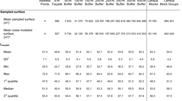
The noise exposure indicator distributions obtained for all the 12 sampling techniques are presented in Tab. 1 and Fig. 3; they are sorted by increasing sampled surface, apart from the administrative surface. The means range from 49.6 dB to 54.5 dB. They are significantly different from each other (P<0.01), except for the address points and the 100-m buffers samples (P=0.46) and for the 150-m buffer and the census blocks sample (P=0.46). The standard deviations range from 7.1 to 4.2. For the façade and buffer techniques, the noise indicators significantly increase when the sampled surface increases, while the noise indicator variances significantly decrease (all P<0.01).
The average Euclidean distance between the address point and its corresponding building is 15.5 m and ranges between 1.2 m and 368 m.
The histograms and the spatial distributions of the exposure indicators for the 50-m and the 400-m buffers are presented in Fig. 4 and Fig. 5, respectively. Not surprisingly, the buildings associated with highest 50 m exposure values (≥55 dB) are located along the main roadways. Conversely, when considering the 400-m indicator, this specific localization of buildings associated with the highest values along the main roadways is no longer observed, but spatial aggregates of medium noise exposition can be noted in the urban fringe.
The histograms and the spatial distributions of the Δ400-50 are presented in Figure 6. The Δ400-50 ranges between -9.4 dB and +22.3 dB, with a mean variation of +3.9 dB. Two thirds of the
7 buildings present a Δ400-50 higher than |3 dB|: 56.5% over +3 dB (n=5 873) and 9.8% under -3 dB (n=1 019). The former appear to be localized very close to the main roadways. A similar behavior of the LAeq,24h exposure variation appears when comparing the two administrative surface
techniques (Census Blocks and Census Block Groups, data not shown).
The multivariate analysis of the relationship between the Δ400-50 and the urban environmental characteristics is summarized in Tab. 2. Adjusted to each other’s, distance to the road, urban type, and population density are significantly and independently associated with the Δ400-50 noise level observed when increasing the neighborhood surface.
DISCUSSION
The urban noise indicators obtained from the four commonly used sampling techniques examined in the present study differ significantly. When the size of the sampled area increases, the mean values increase while the variance decreases. The urban morphology and the structure of the residential environment are both associated with this difference between indicators.
The exclusion from the dataset of all buildings within 400 m from the city limits did not allow for the study of the noise exposure in the peripheral area. However, the high number of residential buildings (10 825), and the suppression of the potential boundary effects, offer a high robustness to the results. The use of a unique validated noise map17 to compute all indicator
controls for measurement bias related to model, building or even city comparisons, and allows a direct comparison between the 4 different sampling techniques.
As no standardized techniques exist to assess residential exposure to noise24, the sampling
techniques were chosen to represent the different approaches that are most commonly used to assess human noise exposure in general living conditions and areas2,4,5,8,9,12,13,14. Outdoor indicators
8 Several definitions of the living area are covered by the four chosen techniques: i) address point indicators represent exposure at a single point supposedly located at the entrance of the building, and often used to quantify the dwelling exposure; ii) façade indicators quantify the acoustic energy reaching the outdoor-indoor interface, assessing dwelling exposure at the closest of the building; iii) Census Blocks and Census Block Groups are administrative areas associated with demographic and socioeconomic characteristics, they allow a fast assessment of outdoor noise levels in the subject’s neighborhood, but reduce the study precision by affecting the same exposure to every subjects belonging to the same administrative division; iv) Buffer indicators deal with immediate living neighborhoods. The straight-line buffer of 1.6 km (one mile), commonly used to define the living neighborhood, appeared to be overestimated for European cities26
, therefore, the 400 m distance was retained as the upper limit of straight-line buffers27
. This value has been proposed to determine the adult “walking neighborhood” reflecting the area where subjects move for most of their daily needs (i.e. grocery shopping, recreational activity, etc…). This choice also reduced the risk of a border effect and over-superposition across the different buffers. Each indicator used in this study present a different conception of outdoor exposure around the dwelling, and no categorical answer can be found to the question of the best indicator. Moreover, the use of a single indicator to represent the truth of outdoor exposure gives a reductionist view of the reality and activity-related variability of human exposure.
The address point technique presents two main differences from the other techniques. First, the noise exposure indicator is calculated on a single sampled pixel, and the distance separating this pixel from its related building varies for each building (from 1.2 m to 368 m). These results match those obtained by Cayo & Talbot28
and by Bonner et al.29
for U.S. urban areas. As a consequence, this pixel is often closer to the road than to its related building, most likely affecting higher noise levels than the façade sampling. Second, the address point technique is
9 highly dependent on the scale definition chosen for the used pixels: the higher the model's definition, the smaller surface the address point associated with it. In a recent study, Eriksson et al.30 also found differences between address points and other sampling techniques, with address points giving significantly different exposure values than façade samplings. Consequently, the use of address points introduced an uncertainty in exposure quantification with a hardly predictable order of magnitude.
Not surprisingly, the variability of the noise exposure indicators appears to be inversely associated with the size of the sample area. Indeed, the number of the sampled pixels increases with the size of the area, and so the standard error of the means decreases. The lower noise levels are obtained using the façade technique, which deals with the smallest and closest sampling surface area around the buildings. It could be seen as the actual environment/building interface and is considered to be directly related to the indoor noise levels31,32,33. This technique is mainly
used to estimate the level of noise exposure2,4,5,8,12 despite the fact that the urban living area is not
limited to indoor home space26,34,35. Indeed, many recreational, physical or commercial activities
happen in the vicinity of the dwelling, especially for non-active subgroups of the population36,37.
Despite statistical significance, differences between noise exposure indicators should also be considered from an acoustical point of view. A |3 dB| difference, corresponding to a doubling of the acoustical energy, could be considered as the smallest relevant value for acoustical significance in environmental noise exposure situation. Therefore, the average increase of +3.9 dB when going from a 50 m to a 400 m neighborhood could be considered as significant. Previous studies have shown a relationship between noise exposure level and urban morphology38,39
. The significant increase of the noise level with the size of the buffers could then be partially explained by the consequence of the progressive modification of the neighborhood structure, especially the inclusion of a higher number of noise sources or of a higher number of
10 areas close to these sources. Furthermore, this increase is not homogeneous between buildings; some of them exhibit a high decrease of their affected noise level, up to nearly -10 dB, while some others exhibit a significant increase higher than +20 dB. These heterogeneous differences seem to be spatially structured, conditioned by environmental factors such as distance toward sources and urban morphology. Indeed, low noise exposure variations are observed in the urban fringe, which often correspond to the individual housing Census block.
The results have been obtained for a medium-sized European city with no major environmental noise sources and moderate noise levels17,18. The city however presents a wide range of noise
level across its area, which leads to a mosaic of exposure situations. In this context, the question of the indice choice appears to be more relevant than in situation where major noise sources (Highways, Airport) could induce more homogeneous exposure areas. Two previous studies conducted in Besançon have indicated that a significant part of the population could suffer from important outdoor nighttime exposure18, and that schoolchildren cognition could be impacted by
outdoor noise exposure40, with a potential impact of the neighborhood socio-economic level. The
two main characteristics of our study are the nature of the noise sources and the particular morphology of Besançon, with a mostly pedestrian old historical center surrounded by areas of more recent development separated by a dense and irregular network of small roadways. This urban morphology is typical of European cities and in accordance with the recent European tendency to limit the urban center access to pedestrian and public transport only. While this morphology eases the comparisons of our results with other similar European cities, this does not allow our results to be compared with more recent non-European cities. In such cities with a regular city block and road network pattern, the urban structure could modify the observed influence of the area size or the urban morphology. If the city blocks are smaller than the areas
11 that define the living neighborhoods, this could result in sampling a repetitive urban morphology, thereby attenuating or erasing the effect observed in this study.
Two consequences should be stated about the influence of the indicator choice on the noise levels. First, exposure level comparisons between studies should be made very cautiously and should consider the types of sampling techniques used. Second, in Environmental Epidemiology, the exposure assessment is a key point in the design and the quality of the study. Outdoor noise exposure values have been shown to be highly influenced by the chosen sampling techniques. Different choices can lead to different (mis)classifications of each subject's exposure level. Thus, these errors in classification can be differential when considering the influence of environment characteristics. The potential bias on the estimated relationships between noise and health is very difficult to predict, both in the direction and the magnitude of the effect.
Based on this study’s findings, no definitive conclusion can be drawn about the best definition (if any) of the area representing the residential noise exposure. Each indicator corresponds to a different definition of the neighborhood, and assesses different activity-related exposure situations. An alternative for a better understanding and representation of the actual residential exposure could be the use of synthetic time-location combination indicators. Daily exposure could be defined by the association of i) the 400-m noise exposure for the daytime, ii) the 50-m or 100-m noise exposure for the evening, and iii) the façade exposure for the night-time. It is however important to keep in mind that the use of a single indicator, or even a single synthetic indicator, for assessing exposure does not fit with the variability of individual behavior and exposure situation. The definition of the best sampling area should integrate the aim of the exposure quantification and the true living neighborhood of the subject according to its living habits, mobility and socio-economical level. The definition appears to be of great influence when considering specific sensitive subgroups, such as schoolchildren2,18, elders41,42, or pregnant
12 women1,43, who are considered the most at risk and whose mobility and activity patterns differ7,44,45
from the rest of the population. Ideally, the exposure indicator should be individually designed to account for individual variability instead of current population approach. This level of precision is still nearly impossible to access for most investigators. However, future eco-epidemiological studies would be greatly improved by the development of new tools and techniques allowing the achievement of such precision.
The results of this study support the fact that the size and the spatial structure of the local living neighborhood matter when assessing residential exposure to urban noise. While no standardized technique has been officially appointed, the sampling techniques should be carefully chosen, keeping in mind influences of environmental factors. The potential impact of assessment choice on the observed relationships between noise, health and others factors, such as socio-economic status, need to be explored to optimize both population exposure and the risk assessment process.
ACKNOWLEDGMENT
Quentin Tenailleau is a Ph.D. student supported by a grant from the city of Besançon. The authors would like to thank the city services, the urban community of Besançon (CAGB), the Besançon Urban Development Agency (AUDAB) and the Departemental Public Works Directorate (DDE) for their technical support.
13 REFERENCES
1. Committee on Environmental Health. Noise: A Hazard for the Fetus and Newborn. Pediatrics 100, 724–727 (1997).
2. Stansfeld, S. A. et al. Aircraft and road traffic noise exposure and children’s mental health. J. Environ. Psychol.
29, 203–207 (2009).
3. Van Kempen, E. E. M. M. et al. The association between noise exposure and blood pressure and ischemic heart disease: a meta-analysis. Env. Health Perspect 110, 307–17 (2002).
4. Babisch, W., Beule, B., Schust, M., Kersten, N. & Ising, H. Traffic noise and risk of myocardial infarction.
Epidemiology 16, 33–40 (2005).
5. De Kluizenaar, Y., Gansevoort, R. T., Miedema, H. M. E. & de Jong, P. E. Hypertension and road traffic noise exposure. J Occup Env. Med 49, 484–92 (2007).
6. Klepeis, N. E. et al. The National Activity Pattern Survey (NHAPS) : a ressource for assessing exposure to environmental pollutants. J. Expo. Anal. Environ. Epidemiol. 11, 231–252 (2001).
7. European Commission. How Europeans spend their time. Everyday life of women and men. (European Commission, 2004).
8. Murphy, E., King, E. A. & Rice, H. J. Estimating human exposure to transport noise in central Dublin, Ireland.
Environ. Int. 35, 298–302 (2009).
9. Selander, J. et al. Long-term exposure to road traffic noise and myocardial infarction. Epidemiology 20, 272–9 (2009).
10. Beelen, R. et al. Mapping of background air pollution at a fine spatial scale across the European Union. Sci.
Total Environ. 407, 1852–1867 (2009).
11. Bodin, T. et al. Road traffic noise and hypertension: results from a cross-sectional public health survey in southern Sweden. Env. Health 8, 38 (2009).
12. Ising, H., Lange-Asschenfeldt, H., Moriske, H.-J., Born, J. & Eilts, M. Low frequency noise and stress: bronchitis and cortisol in children exposed chronically to traffic noise and exhaust fumes. Noise Health 6, 21–8 (2004).
13. Gan, W. Q., McLean, K., Brauer, M., Chiarello, S. A. & Davies, H. W. Modeling population exposure to community noise and air pollution in a large metropolitan area. Environ. Res. 116, 11–16 (2012).
14. Havard, S., Reich, B. J., Bean, K. & Chaix, B. Social inequalities in residential exposure to road traffic noise: An environmental justice analysis based on the RECORD Cohort Study. Occup. Environnemental Med. 68, 366–374 (2011).
15. National Institute of the Statistics and the Economic Studies. Populations légales 2008 de Besançon. (2008). at
<http://www.insee.fr/fr/ppp/bases-de-donnees/recensement/populations-legales/commune.asp?annee=2008&depcom=25056>
16. National Institute of the Statistics and the Economic Studies. Urban units of more than 100,000 inhabitants in 2009. (2010). at <http://www.insee.fr/en/themes/tableau.asp?reg_id=0&ref_id=nattef01204>
17. Pujol, S., Houot, H., Antoni, J. P. & Mauny, F. Linking traffic and noise models to explore spatio-temporal distribution of noise pollution: an example in Besançon (France). in Int. Inst. Acoust. Vib. (2012).
18. Pujol, S. et al. Urban ambient outdoor and indoor noise exposure at home: A population-based study on schoolchildren. Appl. Acoust. 73, 741–750 (2012).
19. Houthuijs, D. et al. WP3 - Noise Exposure Assessment. 32 (European Network on Noise and Health, 2010). 20. National Institute of the Statistics and the Economic Studies. Definition of ‘Statistical Block’. (2013). at
<http://www.insee.fr/en/methodes/default.asp?page=definitions/ilot.htm>
21. National Institute of the Statistics and the Economic Studies. Definition of ‘IRIS’. (2013). at <http://www.insee.fr/en/methodes/default.asp?page=definitions/iris.htm>
22. Houot, H. Geographycal approach of annoyance due to noise transportation. in Proc. Internoise 2000 4 p (2000).
23. National Institute of the Statistics and the Economic Studies. Results of the Population Census - 2009. (2009). at <http://www.recensement.insee.fr/basesInfracommunales.action>
24. Murphy, E. & King, E. A. Strategic environmental noise mapping: Methodological issues concerning the implementation of the EU Environmental Noise Directive and their policy implications. Environ. Int. 36, 290– 298 (2010).
25. Nieuwenhuijsen, M., Paustenbach, D. & Duarte-Davidson, R. New developments in exposure assessment: The impact on the practice of health risk assessment and epidemiological studies. Environ. Int. 32, 996–1009 (2006).
14
26. Smith, G., Gidlow, C., Davey, R. & Foster, C. What is my walking neighbourhood? A pilot study of English adults’ definitions of their local walking neighbourhoods. Int. J. Behav. Nutr. Phys. Act. 7, 34–42 (2010). 27. Forsyth, A., Hearts, M., Oakes, J. & Schmitz, K. Design and destinations: factors influencing walking and total
physical activity. Urban Stud. 45, 1973–1996 (2008).
28. Cayo, M. R. & Talbot, T. O. Positional error in automated geocoding of residential addresses. Int. J. Health
Geogr. 2, 10 (2003).
29. Bonner, M. R. et al. Positional Accuracy of Geocoded Addresses in Epidemiologic Research. Epidemiology 14, 408–412 (2003).
30. Eriksson, C., Nilsson, M. E., Stenkvist, D., Bellander, T. & Goran, P. Residential traffic noise exposure assessment: application and evaluation of European Environmental Noise Directive maps. J. Expo. Sci.
Environ. Epidemiol. 1–8 (2012).
31. ISO 1996-2:2007. Acoustics. Description, assessment and measurement of environmental noise - Part 2:
Determination of environmental noise levels. Int. Organ. Stand. (2006).
32. WHO Europe. Night Noise Guidelines for Europe. (World Health Organization - Regional Office for Europe, 2009).
33. Pirrera, S., Valck, E. D. & Cluydts, R. Nocturnal road traffic noise assessment and sleep research: The usefulness of different timeframes and in- and outdoor noise measurements. Appl. Acoust. 72, 677 – 683 (2011).
34. Galster, G. On the Nature of Neighbourhood. Urban Stud. 38, 2111–2124 (2001).
35. Chaix, B., Merlo, J., Evans, D., Leal, C. & Havard, S. Neighbourhoods in eco-epidemiologic research: Delimiting personal exposure areas. A response to Riva, Gauvin, Apparicio and Brodeur. Soc. Sci. Med. 69, 1306–1310 (2009).
36. Scott, M. M., Evenson, K. R., Cohen, D. A. & Cox, C. E. Comparing Perceived and Objectively Measured Access to Recreational Facilities as Predictors of Physical Activity in Adolescent Girls. J. Urban Health 84, 346–359 (2007).
37. Prins, R., Oenema, A., van der Horst, K. & Brug, J. Objective and perceived availability of physical activity opportunities: differences in associations with physical activity behavior among urban adolescents. Int. J.
Behav. Nutr. Phys. Act. 6, 70 (2009).
38. Montalvào Guedes, I. C., Bertoli, S. R. & Zannin, P. H. T. Influence of urban shapes on environmental noise: A case study in Aracaju - Brazil. Sci. Total Environ. 412-413, 66 – 76 (2011).
39. Wang, B. & Kang, J. Effects of urban morphology on the traffic noise distribution through noise mapping: A comparative study between UK and China. Appl. Acoust. 72, 556 – 568 (2011).
40. Pujol, S. et al. Association between Ambient Noise Exposure and School Performance of Children Living in An Urban Area: A Cross-Sectional Population-Based Study. J. Urban Health 1–16 (2013). doi:10.1007/s11524-013-9843-6
41. Wang, Z. & Lee, C. Site and neighborhood environments for walking among older adults. Health Place 16, 1268–1279 (2010).
42. Parra, D. C., Gomez, L. F., Fleischer, N. L. & David Pinzon, J. Built environment characteristics and perceived active park use among older adults: Results from a multilevel study in Bogota. Health Place 16, 1174–1181 (2010).
43. Hohmann, C. et al. Health effects of chronic noise exposure in pregnancy and childhood: A systematic review initiated by \ENRIECO\. Int. J. Hyg. Environ. Health 216, 217 – 229 (2013).
44. Klepeis, N. E., Tsang, A. M., Behar, J. V. & U.S. Environmental Protection Agency. Analysis of the National
Human Activity Pattern Survey (NHAPS) Respondents from a Standpoint of Exposure Assessment. (1995).
45. National Institute of the Statistics and the Economic Studies. Depuis 11 ans, moins de tâches ménagères, plus d’Internet. INSEE Prem. 4 (2011).
15 FIGURES
Figure 1. Example of the sampling techniques
16
Figure 3. Boxplots of the average LAeq,24h level distributions evaluated for each sampling
17
18
19
Figure 6. Assigned LAeq,24h level evolution between the 50-m buffer sampling and the 400-m
buffer sampling (Δ400-50, n=10 825)
20
Table 1. Average LAeq,24h (in dB) according to the surface of the sampling techniques (n=10 825)
Address Points 6-m Façade 50-m Buffer 100-m Buffer 150-m Buffer 200-m Buffer 250-m Buffer 300-m Buffer 350-m Buffer 400-m Buffer Census Blocks Census Block Groups Sampled surface
Mean sampled surface
(m²) 4 566 7 833 31 375 70 624 125 581 196 247 282 618 384 700 502 488 70 783 994 201
Mean noise modeled surface (m²)* 4 507 5 734 24 120 55 376 99 916 157 645 227 374 313 033 410 203 63 145 842 440 LAeq24H Mean 51.0 49.6 50.4 51.4 52.1 52.7 53.2 53.6 53.9 54.2 52.3 54.5 SD† 7.1 6.5 6.3 6.1 5.9 5.8 5.6 5.3 5.1 4.9 5.6 4.2 Min 25.0 24.7 25.6 27.6 30.7 32.7 34.6 36.0 37.1 39.2 39.4 46.8 Max 72.0 71.8 69.1 66.4 65.3 64.4 63.6 63.0 62.7 62.2 67.2 62.6 1st quartile 47.0 45.4 46.3 47.1 47.7 48.3 49.0 50.0 51.2 52.0 48.0 51.0 Median 51.0 49.4 50.0 50.9 52.1 53.3 54.3 55.1 55.5 55.6 52.6 56.3 3rd quartile 55.0 53.8 54.5 56.1 57.1 57.5 57.6 57.7 57.7 57.8 56.5 57.5
* Mean noise modeled surface = mean sampled surface - built surface in the sampled area. †Standard Deviation.
Table 2. Multilevel analysis of the LAeq,24h level variation for an increasing of the buffer sampling
21 Level Variable β 95% CI* P-value
Building Distance to nearest road (for
+100 m) 4.8 4.3 – 5.3 < 0.01 Distance to nearest main road
(for +100 m) 1.9 1.5 – 2.2 < 0.01 Census
Blocks
Urban typology †
(Ref : Individual Housing) < 0.01 Densely Urbanized Area 0.2 -1.3 – 1.7 Social Housing 1.6 0.5 – 2.7 Mixed Residential Area 0.8 -0.2 – 1.8 Activity Center -2.2 -4.0 – -0.5 C. Block
Groups
Density †
(for +1000 hab/Km²) 0.1 0.0 – 0.2 < 0.01 * 95% Confidence Interval. † Variables are adjusted on the distance to the nearest road.
Noise exposure variation observed when increasing the sampled surface is 1.6 dB higher in social housing Census Blocks than in individual housing Census Blocks, independently of the distance to the road.