Land use change and El Niño-Southern Oscillation drive decadal carbon balance shifts in Southeast Asia

HAL Id: hal-01806789

https://hal.archives-ouvertes.fr/hal-01806789

Submitted on 17 Sep 2020

HAL is a multi-disciplinary open access

archive for the deposit and dissemination of

sci-entific research documents, whether they are

pub-lished or not. The documents may come from

teaching and research institutions in France or

abroad, or from public or private research centers.

L’archive ouverte pluridisciplinaire HAL, est

destinée au dépôt et à la diffusion de documents

scientifiques de niveau recherche, publiés ou non,

émanant des établissements d’enseignement et de

recherche français ou étrangers, des laboratoires

publics ou privés.

Distributed under a Creative Commons Attribution| 4.0 International License

decadal carbon balance shifts in Southeast Asia

Masayuki Kondo, Kazuhito Ichii, Prabir Patra, Joseph Canadell, Benjamin

Poulter, Stephen Sitch, Leonardo Calle, Yi Liu, Albert van Dijk, Tazu Saeki,

et al.

To cite this version:

Masayuki Kondo, Kazuhito Ichii, Prabir Patra, Joseph Canadell, Benjamin Poulter, et al.. Land

use change and El Niño-Southern Oscillation drive decadal carbon balance shifts in Southeast Asia.

Nature Communications, Nature Publishing Group, 2018, 9, pp.1154. �10.1038/s41467-018-03374-x�.

�hal-01806789�

Land use change and El Niño-Southern Oscillation

drive decadal carbon balance shifts in Southeast

Asia

Masayuki Kondo

1,2

, Kazuhito Ichii

1,2,3

, Prabir K. Patra

2,22

, Joseph G. Canadell

4

, Benjamin Poulter

5,6

,

Stephen Sitch

7

, Leonardo Calle

5

, Yi Y. Liu

8,9

, Albert I.J.M. van Dijk

10

, Tazu Saeki

3

, Nobuko Saigusa

3

,

Pierre Friedlingstein

7

, Almut Arneth

11

, Anna Harper

7

, Atul K. Jain

12

, Etsushi Kato

13

, Charles Koven

14

,

Fang Li

15

, Thomas A.M. Pugh

11,16

, Sönke Zaehle

17

, Andy Wiltshire

18

, Frederic Chevallier

19

, Takashi Maki

20

,

Takashi Nakamura

21

, Yosuke Niwa

20

& Christian Rödenbeck

17

An integrated understanding of the biogeochemical consequences of climate extremes and

land use changes is needed to constrain land-surface feedbacks to atmospheric CO

2

from

associated climate change. Past assessments of the global carbon balance have shown

particularly high uncertainty in Southeast Asia. Here, we use a combination of model

ensembles to show that intensified land use change made Southeast Asia a strong source of

CO

2

from the 1980s to 1990s, whereas the region was close to carbon neutral in the 2000s

due to an enhanced CO

2

fertilization effect and absence of moderate-to-strong El Niño

events. Our

findings suggest that despite ongoing deforestation, CO

2

emissions were

sub-stantially decreased during the 2000s, largely owing to milder climate that restores

photo-synthetic capacity and suppresses peat and deforestation

fire emissions. The occurrence of

strong El Niño events after 2009 suggests that the region has returned to conditions of

increased vulnerability of carbon stocks.

DOI: 10.1038/s41467-018-03374-x

OPEN

1_{Center for Environmental Remote Sensing (CEReS), Chiba University, Chiba 263-8522, Japan.}2_{Department of Environmental Geochemical Cycle Research,}

Japan Agency for Marine-Earth Science and Technology, Yokohama 236-0001, Japan.3_{Center for Global Environmental Research, National Institute for}

Environmental Studies, Tsukuba 305-8506, Japan.4Global Carbon Project, CSIRO Oceans and Atmosphere, Canberra, ACT 2601, Australia.5Institute on

Ecosystems and Department of Ecology, Montana State University, Bozeman, MT 59717, USA.6Biospheric Science Laboratory, NASA Goddard Space Flight

Center, Greenbelt, MD 20771, USA.7University of Exeter, Exeter EX4 4QF, UK.8School of Geography and Remote Sensing, Nanjing University of

Information Science and Technology, Nanjing 210044, China.9ARC Centre of Excellence for Climate Systems Science and Climate Change Research Centre,

University of New South Wales, Sydney, NSW 2052, Australia.10Fenner School of Environment and Society, Australian National University, Canberra, ACT

0200, Australia.11Institute of Meteorology and Climate Research, Environmental Atmospheric Research (IMK-IFU), Karlsruhe Institute of Technology (KIT),

Kreuzeckbahnstraße 19, 82467 Garmisch-Partenkirchen, Germany.12Department of Atmospheric Sciences, University of Illinois at Urbana-Champaign,

Urbana, IL 61801, USA.13Institute of Applied Energy, Tokyo 105-0003, Japan.14Earth Sciences Division, Lawrence Berkeley National Laboratory, Berkeley,

CA 94720, USA.15International Center for Climate and Environmental Sciences, Institute of Atmospheric Physics, Chinese Academy of Sciences, Beijing

100864, China.16School of Geography, Earth and Environmental Science and Birmingham Institute of Forest Research, University of Birmingham,

Birmingham B15 2TT, UK.17Biogeochemical Integration Department, Max Planck Institute for Biogeochemistry, 07701 Jena, Germany.18Met Office Hadley

Centre, Fitzroy Road, Exeter EX1 3PB, UK.19Laboratoire des Sciences du Climat et de l’Environnement (LSCE), CEA CNRS UVSQ, 91191 Gif Sur Yvette, France.

20_{Meteorological Research Institute, Tsukuba 305-0052, Japan.}21_{Japan Meteorological Agency, Tokyo 100-8122, Japan.}22_{Present address: Research and}

Development Center for Global Change (RCGC) Japan Agency for Marine-Earth Science and Technology, Yokohama 236-0001, Japan. These authors contributed equally: Kazuhito Ichii, Prabir K. Patra, Joseph G. Canadell, Benjamin Poulter, Stephen Sitch, Leonardo Calle. Correspondence and requests for

materials should be addressed to M.K. (email:redmk92@gmail.com)

123456789

S

outheast Asia is unique among tropical regions because the

region is highly susceptible to the influence of El

Niño-Southern Oscillation (ENSO)

1, 2

and is subject to highest

deforestation rates in the tropical regions

3–6

. In the recent past,

Southeast Asia experienced large CO

2

emissions, ranging from

0.81 to 1.2 Pg C yr

−1

due to the drought-induced

fires during the

1997/1998 El Niño

7,8

, and a substantial loss of forest area (2.5

Mha in the 1990s)

9

due to forest conversion to oil palm and

rubber tree plantations

10–12

. However, contrary to the intensively

studied Amazon Basin and Congo Basin with permanent plot

sample data

13, 14

, the recent states of net CO

2

flux (balance

between CO

2

uptake and release by the land biosphere) across

Southeast Asia remain highly uncertain. The Fifth Assessment

Report (AR5) of the Intergovernmental Panel on Climate Change

(IPCC) provided a synthesis of the global net CO

2

flux. However,

disregard of land use change (LUC) in the biosphere models (the

bottom-up approach) resulted in an underestimation of CO

2

release for the tropical regions when compared with the

atmo-spheric CO

2

inversions (the top-down approach)

15

. Both climate

and LUC need to be integrated into analyses to adequately

esti-mate the net CO

2

flux and to reconcile results from different

approaches. Such an integrated effort has not been undertaken for

Southeast Asia.

Here we investigate the decadal variability of the net CO

2

flux

(termed Net Biome Production: NBP, the negative sign (–) for a

net sink and the positive sign (+) for a net source) in Southeast

Asia over the period 1980–2009 using an ensemble of seven

terrestrial biosphere model simulations from the TRENDY model

intercomparison project (Supplementary Table

1

), an ensemble of

five atmospheric CO

2

inversions that cover longer than two

decades (Supplementary Tables

2

,

3

) and a remote-sensing-based

annual biomass change estimated by Global Aboveground

Bio-mass Carbon version 1.0 (Supplementary Fig.

1

). We demonstrate

that consideration of LUC processes to biosphere models brings

consistency in interannual and decadal variability of the net CO

2

flux between the bottom-up, top-down and remote-sensing-based

approaches, indicating carbon balance shifts towards a net source

from the 1980s to 1990s, and towards a net sink from the 1990s to

2000s. Subsequently, we quantify the contributions to the decadal

NBP variability from CO

2

fertilization, climatic conditions and

LUC using three sets of TRENDY simulations (Supplementary

Fig.

2

) where biosphere models were forced with varying CO

2

,

climate and historical LUC (TRENDY S3), along with simulations

forced with varying CO

2

and climate (TRENDY S2), and varying

CO

2

only (TRENDY S1). Our results show that increased LUC

emissions during the 1990s was the major factor responsible for

the shift towards a net source between the 1980s and 1990s, and

the enhanced CO

2

fertilization and absence of strong El Niño

events during the 2000s for the shift towards a net sink between

the 1990s and 2000s. The milder climate sustained during the

2000s is of particular importance to a high carbon assimilation by

plant ecosystems in Southeast Asia, inducing a strong net uptake

that cancels a large proportion of CO

2

release from ongoing LUC

in the region.

Results

The effect of LUC on net CO

2

flux. We find agreement in

interannual variability of NBP between the TRENDY S3 and

atmospheric CO

2

inversions for the period 1980–2009, and the

annual biomass change (hereafter,

Δbiomass) for the period

1994–2009, as indicated by high correlations between the three

estimates (r

= 0.67–0.70, p < 0.01, Fig.

1

a; detailed inter-model

comparisons in Supplementary Figs.

3

,

4

). However, this

agree-ment is not found in a comparison with the TRENDY S2, which

indicates continuously strong CO

2

uptake throughout the 30-year

period. The inclusion of LUC (adding LUC to the model forcing

as in TRENDY S3; Supplementary Fig.

5

) changed both the

patterns of the spatial variability of NBP (Fig.

1

b; individual

model results in Supplementary Fig.

6

) as well as the sign of mean

annual NBP from a large sink to a weak source for the period

1980–2009; flux changed from −0.18 ± 0.09 Pg C yr

−1

in the

TRENDY S2 (average ± 1σ as model-by-model variability) to

0.09 ± 0.12 Pg C yr

−1

in the TRENDY S3. This result confirms

that the LUC emissions are a key factor in NBP estimation for

Southeast Asia, as its contribution to NBP is large, so much as to

cancel the CO

2

uptake due to the effect of CO

2

fertilization.

The decadal shifts of net CO

2

flux and attributions. The

inter-decadal mean NBP estimates from the TRENDY S3, atmospheric

CO

2

inversions and

Δbiomass yield a consistent pattern of

dec-adal variability, indicating that an increased net source from the

1980s to the 1990s is largely decreased in the 2000s (Fig.

1

c;

individual model results in Supplementary Fig.

7

). By isolating the

contributions of the effects from CO

2

fertilization, climate and

LUC to NBP using the TRENDY model simulations (Methods),

we found that the shift towards a stronger net source from the

1980s to the 1990s is primarily attributable to the intensifying

LUC (Fig.

1

d; individual model results in Supplementary Fig.

8

a),

which increased the net source from 0.21 ± 0.11 Pg C yr

−1

(the

1980s) to 0.31 ± 0.13 Pg C yr

−1

(the 1990s). In contrast, a reduced

net source (i.e. stronger sink) from the 1990s to the 2000s is

attributed to the effects of CO

2

fertilization and climate

(Fig.

1

d; Supplementary Fig.

8

b, c), with the former inducing

a

change

from

−0.23 ± 0.08 Pg C yr

−1

(the

1990s)

to

−0.28 ± 0.09 Pg C yr

−1

_{(the 2000s), and the latter from 0.09 ±}

0.11 Pg C yr

−1

(the 1990s) to 0.001 ± 0.11 Pg C yr

−1

(the 2000s).

We examine the robustness of these decadal shifts by applying

non-parametric trend tests to the periods 1980–1999 and

1990–2009 (Mann–Kendall and Theil slope tests; Methods).

Using the NBP estimates including individual TRENDY models,

we found that trends of increasing CO

2

uptake for the period

1990–2009 tend to be more statistically significant (p < 0.05) than

those of increasing CO

2

release for the period 1980–1999 (Fig.

2

a).

Further analysis of the individual TRENDY models shows

statistically significant trends of increasing CO

2

release due to

the LUC effect for the period 1980–1999 and of increasing CO

2

uptake in response to the CO

2

fertilization and climate effects for

the period 1990–2009 (Fig.

2

b, c). This multi-model trend

analysis suggests that the decadal NBP shift from the 1990s to

2000s is more robust than that from the 1980s to 1999s, which

means that the CO

2

fertilization and climate conditions in the

2000s are more influential to NBP than the enhanced LUC

activities in the 1990s, distinguishing the 2000s from previous

decades. It is reasonable to expect that the CO

2

fertilization is

partly responsible for the decadal NBP shift from the 1990s to

2000s because atmospheric CO

2

is the main factor driving NBP

towards a net sink via promoting the photosynthetic carbon

fixation

16

_{. The increased CO}

2

fertilization effect in the 2000s

coincides with higher CO

2

concentrations in the 2000s (379 ppm)

than those in the 1980s (346 ppm) and the 1990s (361 ppm,

decadal averages based on

flask sampling data at the Mauna Loa

Observatory: Data—NOAA Earth System Research Laboratory,

https://www.esrl.noaa.gov/gmd/ccgg/trends/data.html

). As for the

climate effect, a net source in the 1980s and 1990s makes a

transition to carbon neutral in the 2000s (Fig.

1

d), implying a

climate favourable for CO

2

uptake in the 2000s.

Weak phase of ENSO in the 2000s. In order to elucidate the

climate effect on NBP in the 2000s, we have analysed mean

annual NBP (i.e. the TRENDY S3, atmospheric CO

2

inversion

1.0 0.5 0.0 1980 1985 1990 1995 2000 2005 2010 NBP (Pg C yr –1) 0.4 0.2 0.0 –0.2 –0.4 1980s 1990s 2000s NBP (Pg C yr –1) 0.4 0.2 0.0 –0.2 –0.4 1980s 1990s 2000s –0.2 Year 0.0 0.3 –0.3 TRENDY S3: CO₂+climate+LUC 0.0 0.3 -0.3 TRENDY S2: CO₂+climate 0.0 0.3 –0.3 NBP (Pg C yr –1 ) TRENDY S1: CO2 only CO2 fertilization effect Climate effect LUC effect TRENDY S2 TRENDY S3 CO2 inversion Δbiomass Net source (+) –0.5 –1.0 NBP (kg C m–2 _yr–1₎ 0.2 0.0

a

b

c

d

NBP (Pg C yr –1 ) Net sink (–) TRENDY S2 TRENDY S3 CO2 inversion Δbiomass 0.8 0.4 0.0 Correlation ( r) 0.70 0.68 0.67

**

**

**

Fig. 1 Interannual and decadal variability of net CO2flux in Southeast Asia for 1980–2009. a Interannual variability of ensemble averaged NBP from the

TRENDY (grey: TRENDY S2; orange: TRENDY S3) and atmospheric CO2inversions (cyan) for the period 1980–2009, and annual biomass change (dashed

green line:Δbiomass) for the period 1994–2009. Shading for the TRENDY and atmospheric CO2inversions represents 1σ variation among models. A

top-right panel shows correlation coefficients (r) between interannual variability of the three NBP estimates for the overlapping periods (1980–2009 for the

TRENDY and atmospheric CO2inversions; 1994–2009 for the TRENDY and Δbiomass, and for the atmospheric CO2inversions andΔbiomass) and

statistical significance is indicated by **p < 0.01. Negative values in NBP represent a net sink, and positive values a net source. b Spatial variability of mean

annual NBP from the TRENDY (seven model ensemble average) for the period 1980–2009. Results are shown for the three simulations: forced with varying

CO2only (left: TRENDY S1); varying CO2and climate (middle: TRENDY S2); and varying CO2, climate and LUC (right: TRENDY S3). Bar graphs represent

mean annual NBP by the TRENDY simulations (grey: TRENDY S1 and S2; orange: TRENDY S3) for the period 1980_{–2009 with error bars representing 1σ}

variation among models.c Decadal NBP budgets from the TRENDY (grey: TRENDY S2; orange: TRENDY S3) and atmospheric CO2inversions (cyan) for

the 1980s, 1990s and 2000s, with error bars representing 1σ variation among models. Decadal budgets from annual biomass changes are shown with

dashed horizontal lines for the 1990s (1994_{–1999) and 2000s (2000–2009). d Decadal variability of the attributing factors to NBP from the TRENDY}

and

Δbiomass) and components of NBP from the TRENDY

model simulations: LUC emissions,

fire emissions and plant CO

2

exchange (difference between CO

2

uptake by photosynthesis and

release by plant respiration and decomposition), in relation to

variability in the Multivariate ENSO Index (MEI: NOAA ESRL,

http://www.esrl.noaa.gov/psd/data/correlation/mei.data

).

CO

2

fluxes between the years that seasonal MEI indicates a

moderate-to-strong tendency towards El Niño (hereafter, intense El Niño

years; Methods) and the rest of years are compared for the three

decades. In the 1980s and 1990s, which are characterized by the

occurrence of strong and persistent El Niño events (e.g. 1982/

1983, 1987/1988, and 1997/1998; Fig.

3

), all the three estimates of

NBP show a clear tendency towards a net loss of CO

2

from the

land in the intense El Niño years compared with the rest of years,

with differences amounting to 0.13–0.14 and 0.14–0.26 Pg C yr

−1

,

respectively (Fig.

4

a, b). In the 2000s, however, no intense El Niño

is indicated by MEI (Fig.

3

), resulting in a near-neutral carbon

balance (Fig.

4

c). This result suggests that, in addition to

enhanced growth from the CO

2

fertilization, the absence of

intense El Niño events is one of the primary causes for the

reduced net emission of Southeast Asia in the 2000s.

The investigation of the intense El Niño years revealed that the

strength of ENSO largely affects plant CO

2

exchange and

fire

emissions, taking into account peat and deforestation

fires (results

from Community Land Model (CLM); Methods). In the 1980s

and 1990s, CO

2

uptake by plants notably shifted towards a net

emission by 0.07–0.09 Pg C yr

−1

in the intense El Niño years

when compared with the remaining years (Fig.

4

a, b). Likewise,

fire emissions by CLM show larger emissions by 0.11 Pg C yr

−1

_in

the intense El Niño years than the rest of years in the 1980s and

by 0.14 Pg C yr

−1

in the 1990s. A caveat is that the strength of

ENSO had negligible influence on the magnitude of fire emissions

simulated without considering the contribution from peat and

deforestation

fires (an ensemble average excluding CLM). In

contrast with plant CO

2

exchange and

fire emissions, the

magnitude of LUC emissions was nearly unchanged regardless

of El Niño conditions. This may be expected, because carbon

removal by deforestation, and wood and crop harvesting is

Net CO2 flux (NBP)

Towards a net sink

LUC effect Towards

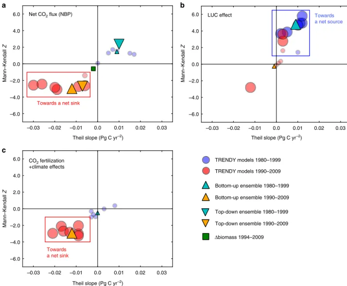
a net source Mann–Kendall Z 6.0 4.0 2.0 0.0 –6.0 –4.0 –2.0 Theil slope (Pg C yr–2) –0.03 –0.02 –0.01 0.0 0.01 0.02 0.03 Mann–Kendall Z 6.0 4.0 2.0 0.0 –6.0 –4.0 –2.0 Theil slope (Pg C yr–2) –0.03 –0.02 –0.01 0.0 0.01 0.02 0.03 CO2 fertilization +climate effects Towards a net sink Mann–Kendall Z 6.0 4.0 2.0 0.0 –6.0 –4.0 –2.0 Theil slope (Pg C yr–2₎ –0.03 –0.02 –0.01 0.0 0.01 0.02 0.03 TRENDY models 1980–1999 TRENDY models 1990–2009 Bottom-up ensemble 1980–1999 Bottom-up ensemble 1990–2009 Top-down ensemble 1980–1999 Top-down ensemble 1990–2009 Δbiomass 1994–2009

a

b

c

Fig. 2 Trends in net CO2flux and its components for the past 30 years. Results of two trend tests (Mann–Kendall and Theil slope tests) on a, net CO2flux

(NBP) from the TRENDY S3 (seven models: blue circles for 1980–1999 and red circles for 1990–2009, and ensemble average: a cyan upper triangle for

1980–1999 and an orange upper triangle for 1990–2009) are shown along with those on the atmospheric CO2inversions (ensemble average: a cyan lower

triangle for 1980−1999 and an orange lower triangle for 1990–2009) and Δbiomass (a green square for 1994−2009). The trend tests on attributing

factors to NBP are illustrated forb, the LUC effect and c, CO2fertilization+climate effects. Size of markers indicates statistical significance of trends: larger

triggered by human activities, which do not directly respond to

climate conditions (with the possible exception of

fire following

deforestation).

Climate sensitivity of CO

2

fluxes in Southeast Asia.

Tempera-ture and water availability to plants (indicated by Standardized

Precipitation Index: SPI) explained most variability in plant CO

2

exchange in Southeast Asia. Among the main meteorological

inputs for the TRENDY models (i.e. temperature, precipitation

and short-wave radiation) and three types of SPI (based on 3-, 6-,

and 9-month moving windows of rainfall accumulation, see

Methods), temperature and SPIs are the variables that show a

significant association with seasonal variability in plant CO

2

exchange: a positive relationship in the former and a negative

relationship in the later (Fig.

5

a; interannual variability of

indi-vidual variables in Supplementary Fig.

9

). The strong

relation-ships found with SPIs suggest that cumulative precipitation over

preceding months is more effective to plant CO

2

exchange than

simple monthly precipitation, and the empirically upscaled eddy

flux data (the FLUXCOM global carbon flux dataset; Methods)

confirm these relationships (Fig.

5

a). Furthermore, both

TRENDY and FLUXCOM data indicate that CO

2

uptake by

plants decreased due to reduced photosynthesis (Gross Primary

Production: GPP) during periods with large increases in

tem-perature and decreases in water availability associated with El

Niño (Fig.

5

b, c, and Supplementary Fig.

10

). The smaller spread

in temperature and SPI anomalies during 2000–2009, compared

to the 1980–1999 period, implies that weak ENSO variability

during the 2000s sustained the high carbon assimilation capacity

of plants in Southeast Asia.

In addition to CO

2

fluxes from plant ecosystems, our results

emphasize

fire emissions as an apparent contributor to net CO

2

flux resulting from severe droughts

17

_{. Particularly, contrasting}

fire emissions between the intense El Niño years and other years

highlights the importance of peat and deforestation

fire emissions

in the carbon balance of Southeast Asia

18

(Fig.

4

). The occurrence

of strong

fire emissions indicated by CLM is found in the years of

negative precipitation anomalies corresponding to the intense El

Niño years (Supplementary Fig.

11

), which is consistent with

fire

emissions estimated by the Global Fire Emissions Database

version 4.1s (GFED4.1s)

19

and reports from

remote-sensing-based and model-remote-sensing-based studies

7, 20, 21

. However, even with the

emissions from peat and deforestation

fires, CO

2

emissions in the

intense El Niño years are still considered as an underestimation of

the reality because the TRENDY models, including CLM, do not

consider emissions from peat oxidative decompositions following

peat

fire events, which could promote even larger CO

2

emissions

during El Niño events

22

.

Discussion

Our results indicate that a synthesis of multiple approaches (i.e.

top-down, bottom-up and remote-sensing-based approaches) is

an effective method to constrain regional carbon balance and to

elucidate causes for major changes in a projection of CO

2

fluxes.

The implementation of LUC processes to biosphere models is

required to estimate net CO

2

flux in Southeast Asia, as indicated

by agreement in the interannual and decadal variability of net

CO

2

flux between the biosphere models, atmospheric CO

2

inversions and

Δbiomass, which has not addressed in the tropical

regions before this study. Our analysis provides new insights for

reconciling the top-down and bottom-up regional

fluxes over the

tropical regions, where wide gaps were reported in the previous

IPCC assessment

15

, and also serves as a useful precedent for

future regional carbon balance assessments by REgional Carbon

Cycle Assessment and Processes (RECCAP)

23

.

The strength of ENSO exerts a strong control on the carbon

balance of Southeast Asia, causing the unique variability in the

decade of 2000s. Along with the recent enhancement of CO

2

fertilization effect

24

, we showed that a milder, less variable,

cli-mate due to the absence of intense El Niño events contributed to

the reduction of CO

2

emissions between the 1990s and 2000s. A

recent synthesis of regional emissions of the greenhouse gases

(GHG) indicates that Southeast Asia is characterized by the

lar-gest emissions not only of CO

2

from ecosystems but also of

agricultural methane and nitrous oxide among the world

regions

25

. Our results suggest that the land response to weak

natural climate variability could serve as a strong mitigation to

CO

2

emissions, even for the world largest ecosystem GHG

emitter.

One aspect not addressed here is the role of La Niña (the

opposite phase to El Niño) in the decadal NBP shift. La Niña can

also induce a milder climate condition, which in turn occasionally

enhances regional CO

2

uptake

26–28

. We emphasize the

sig-nificance of El Niño events in the Southeast Asian carbon balance

because of a difference in the impact on tropical CO

2

fluxes

between the two climate phenomena

29

. As illustrated in Fig.

6

a, b,

linear relationships between seasonal MEI and NBP anomaly

(based on the ensembles of the TRENDY models and

atmo-spheric CO

2

inversions; individual model results in

Supplemen-tary Figs.

12

,

13

and Supplementary Table

4

) demonstrate that

moderate and strong El Niño events (i.e. MEI >1) in the 1980s

and 1990s are directly related to a large net source by the land

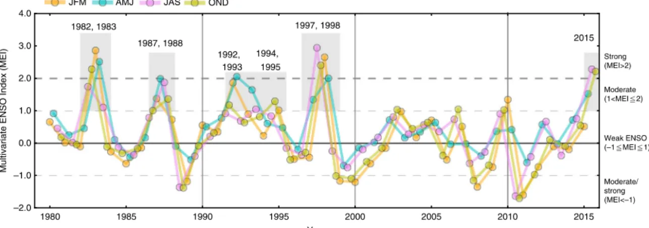
1982, 1983 1987, 1988 1992, 1993 1994, 1995 1997, 1998 2015 Strong (MEI>2) Moderate (1<MEI<2) Moderate/ strong (MEI<–1) Weak ENSO (–1<MEI<1) 4.0 3.0 2.0 1.0 0.0 –1.0 –2.0

Multivariate ENSO Index (MEI)

JFM AMJ JAS OND

1980 1985 1990 1995 2000 2005 2010 2015

Year

Fig. 3 Interannual variability in seasonal Multivariable El Niño-Southern Oscillation Index. Interannual variability in seasonal (3-month averaged, i.e. JFM, AMJ, JAS and OND) Multivariable ENSO Index (MEI). Boundaries for the El Niño and La Niña categorization are indicated by dashed lines, and years correspond to the condition for the intense El Niño years are highlighted by grey shadings (see Methods)

biosphere. In contrast, the data corresponding to La Niña and

weak ENSO events tend to cluster around carbon neutral,

implying that CO

2

uptake during La Niña events (such as years

1984/1995, 1989/1990, and 1989/1990) is less significant

com-pared to CO

2

emissions during El Niño events. Importantly, in

the MEI–NBP relationship, a tendency towards a net source

disappeared during the 2000s (Fig.

6

c). The 2007/2008 La Niña is

one of the strongest events during the past 30 years (Fig.

3

).

However, its contribution to the decadal carbon balance shift in

the 2000s is incomparable to that from the absence of moderate

and strong El Niño events (Fig.

6

e). Given the response of the

land biosphere to El Niño events, we suggest that the dominant

driver of the NBP shift in the 2000s is the absence of moderate

and strong El Niño events, with La Niña events playing a lesser

role.

The absence of moderate-to-strong El Niño events in the 2000s

was a unique case where a natural climate cycle acted to mitigate

CO

2

emissions in Southeast Asia, albeit only for a limited period.

Our estimates of NBP for the period 2010–2016 (see Methods)

indicate net CO

2

emissions comparable to those in the 1980s and

1990s during El Niño events after 2009 such as the 2015/2016 El

Niño (Fig.

6

d). An assessment of climate model simulations

suggest that surface ocean warming over the eastern equatorial

Pacific may lead to an increase in the frequency of intense El

Niño events in the future

30

, reducing the likelihood that natural

climate cycles offer mitigation of CO

2

emissions, and therefore

leading to stronger positive carbon-climate feedback. In the long

term, national-level efforts for forest conservation and ecosystem

management, such as the Reduce Emissions from Deforestation

and forest Degradation (REDD+) project, are critical to

pro-tecting the current CO

2

sink capacity of the Southeast Asia

31,32

.

Methods

Sign convention for net CO2flux. In this study, we chose the sign convention for

net CO2flux that is commonly used in top-down analyses: the negative sign (–) for

a net sink and the positive sign (+) for a net source. This sign convention is consistently used throughout the analysis regardless of the TRENDY models,

atmospheric CO2inversions and annual biomass change, and it is also applied not

only to NBP but also to plant CO2exchange. It should be noted that a common

sign convention for these variables in bottom-up analyses are opposite to this study33.

Bottom-up net CO2flux. Outputs from the TRENDY model intercomparison

project version 2 (TRENDY)34,35were used to calculate the bottom-up net CO2

flux. Simulations of the biosphere models that participated in the TRENDY were

prepared with a consistent forcing dataset: (1) atmospheric CO2concentration for

1860–2012 based on ice-core measurements and stationary observations from

NOAA, (2) climate dataset for 1901–2012 based on a merging between Climate

Research Unit (CRU) TS3.2 0.5° × 0.5° monthly climate data36_{and National}

Centers for Environmental Prediction (NCEP) and National Center for Atmo-spheric Research Reanalysis 2.5° × 2.5° 6-hourly climate data37_{, and (3) 0.5° × 0.5°}

gridded annual LUC dataset for 1860–201238_.

The TRENDY models were simulated under three protocols: a protocol that

considers variability in atmospheric CO2(TRENDY S1); a protocol that considers

variability in CO2and climate (TRENDY S2); and a protocol that considers

variability in CO2, climate and historical LUC (TRENDY S3). For each protocol,

the modelsfirst established an equilibrium state of carbon balance by a spin-up

run, which is forced with the 1860 CO2concentration (287.14 ppm), recycling

climate mean and variability from the early decades of the twentieth century (i.e. 1901–1920) and constant 1860 crops and pasture distribution. Then, simulations for two transient periods were conducted. For the period 1861–1900, the models

were forced with varying CO2concentration and recycling climate (as in spin-up)

in the TRENDY S1 and S2, and in addition varying LUC in the TRENDY S3. After the 1861–1900 period, the models were consecutively run for the 1901–2012 period

with varying CO2concentration and recycling spin-up climate in the S1, varying

CO2concentration and climate in the TRENDY S2 and S3, and varying LUC in the

TRENDY S3. A summary of the forcing data configuration for these simulations is

shown in Supplementary Fig.2.

Among the participating models, we selected seven models that satisfy necessary criteria for the analyses such that models provide monthly NBP outputs for all three simulations and an explicit output of annual LUC emissions.

Specifically, they are the CLM version 4.539_{, Integrated Science Assessment}

Model40, Joint UK Land Environment Simulator (JULES) version 3.241,

Lund-Potsdam-Jena DGVM wsl (LPJ)42, LPJ-GUESS43, Orchidee-CN (O-CN)44and

Vegetation Integrative SImulator for Trace gases (VISIT)45_{. Spatial resolutions of}

the TRENDY model outputs are not consistent among these seven models;fine

resolutions were used in some models and coarse resolution in others

(Supplementary Table1). For models whose outputs were submitted with coarse

spatial resolution, we rescaled grids so that all seven model outputs have the consistent spatial resolution of 0.5° × 0.5°.

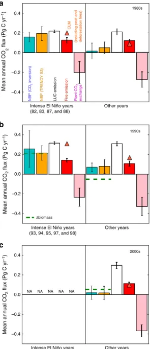
Mean annual CO 2 flux (Pg C yr –1) 0.4 0.2 0.0 –0.2 –0.4 NBP (CO 2 inversion)

NBP (TRENDY S3) LUC emission Fire emission Plant CO

2

exchange

(including peat and deforestation fires)

1980s

Intense El Niño years (82, 83, 87, and 88) Other years 1990s Mean annual CO 2 flux (Pg C yr –1) 0.4 0.2 0.0 –0.2 –0.4

Intense El Niño years (93, 94, 95, 97, and 98) Other years Δbiomass

b

NA NA NA NA NA 2000s

c

Intense El Niño years Other years

Mean annual CO 2 flux (Pg C yr –1 ) 0.4 0.2 0.0 –0.2 –0.4 CLM

a

Fig. 4 In_{fluence of the intense El Niño years on annual CO}2fluxes of the

past three decades. Comparison of mean annual CO2fluxes (NBP, LUC

emissions,fire emissions and plant CO2exchange) between the intense El

Niño years and rest of years fora the 1980s, b the 1990s and c the 2000s.

Mean annual NBP from the atmospheric CO2inversions (cyan) and

TRENDY S3 (orange) are shown for the three decades, andΔbiomass

(dashed green horizontal line) for the 1990s (1994_{–1999) and the 2000s}

(2000–2009). Component fluxes such as LUC emissions (white) and fire

emissions (red), and plant CO2exchange (pink) are the estimates from the

TRENDY S3. Fire emissions considering the attribution from peat and

deforestationfires (the CLM model; orange triangles) are shown separately

from an ensemble average offire emissions by the other models. Error bars

LUC emissions. The LUC forcing for the TRENDY models provides gridded historical transitions of land use, based on annual changes of cropland and pas-tureland area, and wood harvest from the UN Food and Agricultural Organization (FAO) national statistics. Historical changes in annual area of cropland and

pastureland were determined by the HistorY Database of the global Environment

(HYDE) model version 3.146, which takes the FAO national statistics for cropland

and pastureland as the main input source, and spatializes the statistics at the spatial resolution of 5′ × 5′ using allocation algorithms and time-dependent weighting

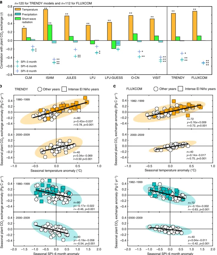
CLM ISAM JULES LPJ LPJ-GUESS O-CN VISIT TRENDY FLUXCOM

Temperature Precipitation Short-wave radiation

Correlation with plant CO

2 exchange ( r) 0.4 0.2 0.0 –0.2 –0.4 0.6 0.8 –0.6 –0.8 Seasonal plant CO 2 exchange anomaly (Pg C yr –1 ) 0.4 0.2 0.0 –0.2 –0.4

Seasonal temperature anomaly (°C)

–1.0 –0.5 0.0 0.5 1.0 0.4 0.2 0.0 –0.2 –0.4

b

TRENDY Other years Intense El Niño years FLUXCOM Other years Intense El Niño years

Seasonal plant CO 2 exchange anomaly (Pg C yr –1 ) 0.4 0.2 0.0 –0.2 –0.4 0.4 0.2 0.0 –0.2 –0.4

Seasonal SPI–6 month anomaly

–1.0 –0.5 0.0 0.5 1.0

–1.5

–2.0 1.5 2.0

a

_{n =120 for TRENDY models and n =112 for FLUXCOM}

Seasonal plant CO 2 exchange anomaly (Pg C yr –1) 0.4 0.2 0.0 –0.2 –0.4 0.4 0.2 0.0 –0.2 –0.4

Seasonal temperature anomaly (°C)

–1.0 –0.5 0.0 0.5 1.0

c

Seasonal plant CO 2 exchange anomaly (Pg C yr –1 ) 0.4 0.2 0.0 –0.2 –0.4 0.4 0.2 0.0 –0.2 –0.4

Seasonal SPI–6 month anomaly

–1.0 –0.5 0.0 0.5 1.0 –1.5 –2.0 1.5 2.0 1980–1999 2000–2009 2000–2009 1980–1999 1982–1999 2000–2009 2000–2009 1982–1999 n = 80 y = 0.43x + 0.037 r = 0.78, p<0.001 n = 40 y = 0.34x – 0.069 r = 0.50 p<0.001 n = 80 y = –0.17x – 0.022 r = –0.46, p<0.001 n = 40 y = –0.19x – 0.058 r = –0.54, p<0.001 n = 72 y = 0.16x + 0.009 r = 0.72, p<0.001 n = 40 y = 0.14x – 0.017 r = 0.75, p<0.001 n = 72 y = –0.10x + 0.002 r = –0.63, p<0.001 n = 40 y = 0.04x – 0.011 r = –0.42, p<0.001 SPI–3 month SPI–6 month SPI–9 month

*

*

*

*

**

**

**

**

**

**

**

**

**

**

**

**

**

**

**

**

**

**

*

**

**

**

**

**

**

Fig. 5 Climate sensitivity of seasonal plant CO2exchange by the biosphere models and empirical upscaling.a Correlation coefficients (r) in relationship

between seasonal anomalies of plant CO2exchange induced by the climate effect (TRENDY S2–S1) and climate variables (temperature, precipitation,

short-wave radiation and three types of SPIs) for the period 1980−2009. Results are shown for seven individual TRENDY models and the ensemble of the

TRENDY and FLUXCOM data. Statistical significances are indicated by **p < 0.01 and *p < 0.05. Relationships between seasonal anomalies of plant CO2

exchange and temperature, and SPI–6 months for the periods 1980–1999 and 2000–2009, for b the TRENDY and c FLUXCOM. All relationships are shown

along with the 95% con_{fident ellipses and linear regressions. Square markers indicate data corresponding to the intense El Niño years and circle markers to}

maps based on global historical population density, soil suitability, distance to rivers, lakes, slopes and biome distributions. The HYDE cropland and pastureland status were then combined with the wood harvest status based on the FAO national wood harvest statistics in order to extend global land use patterns, including transitions of cropland, pastureland, primary and secondary lands (an extended

version of HYDE)38_{. First, the gridded cropland and pastureland area from the}

HYDE model was rescaled from 5′ × 5′ to 0.5° × 0.5° resolution, and at the same

time, fractions occupied by cropland and pastureland was calculated for each rescaled grid cell. By subtracting fractions of cropland and pastureland (and water/ ice if any) from each grid cell, fractions of natural vegetation (primary or secondary lands) was also determined for each grid cell. Distinction between primary and secondary lands (previously disturbed by human activities or not) and fractions of these land types occupied in each grid cell were determined based on the spatialized FAO wood harvest data with empirically estimated biomass density maps produced

n = 40, y = 0.09x – 0.04 r = 0.78, p < 0.001 Seasonal NBP anomaly (Pg C yr –1) 1.0 0.5 0.0 –0.5 –1.0 Seasonal MEI –3.0 –2.0 –1.0 0.0 1.0 2.0 3.0 4.0 La Niña n = 40,y = 0.52x – 0.06 r = 0.33, p < 0.05 TRENDY S3 CO₂ inversion 1.0 0.5 0.0 –0.5 –1.0 Seasonal MEI –3.0 –2.0 –1.0 0.0 1.0 2.0 3.0 4.0 2000s 1980s 1990s Seasonal MEI –3.0 –2.0 –1.0 0.0 1.0 2.0 3.0 4.0 1.0 0.5 0.0 –0.5 –1.0 n = 40, y = 0.12x – 0.01 r = 0.73, p < 0.001 n = 40, y = 0.06x – 0.07, r = 0.42, p < 0.05 n = 40, y = 0.06x – 0.06 r = 0.28, p = 0.08 n = 40, y = 0.05x – 0.05 r = 0.23, p=0.08

a

b

c

Moderate/

strong Weak ENSO

Strong Seasonal NBP anomaly (Pg C yr –1) Seasonal NBP anomaly (Pg C yr –1 ) n = 3 n = 14 n = 13 n = 7 n = 3 n = 2 n = 11 n = 15 n = 7 n = 5 0.0 –0.2 0.2 0.4 0.0 –0.2 0.2 0.4 n = 4 n = 15 n = 19 n = 2 n = 0 0.0 –0.2 0.2 0.4 (Pg C yr –1) (Pg C yr –1) (Pg C yr –1) –3.0 1.0 0.5 0.0 –0.5 –1.0 Seasonal NBP anomaly (Pg C yr –1) Seasonal MEI –2.0 –1.0 0.0 1.0 2.0 3.0 4.0 n = 28, y = 0.11x – 0.03 r = 0.91, p < 0.001 n = 28, y = 0.06x – 0.01 r = 0.69, p < 0.001 2010–2016

d

n = 3 n = 8 n = 10 n = 4 n=3 0.0 –0.2 0.2 0.4 (Pg C yr –1) Reduction of CO2 emissions

due to the absence of moderate and strong El Niño events

Increase in CO2 uptake

due to the occurence of a strong La Niña event

1980s–1990s _2000s NBP (Pg C yr –1 ) 0.3 0.2 0.1 0.0 –0.1 –0.2 El Niño events (moderate/strong) La Niña events (moderate/strong)

e

–0.19 Pg C yr–1 –0.01 Pg C yr–1 La Niña Moderate/ strong Moderate Weak ENSO Strong

La Niña Moderate/ strong

Moderate Weak ENSO Strong La Niña

Moderate/ strong

Moderate Weak ENSO Strong

El Niño Moderate

El Niño El Niño

at the spatial resolution of 0.5° × 0.5° from Miami-LU model47. Both the HYDE and extended HYDE models assume a strong association between land use and

human population48_{. Thus, interannual variability of the land use status for the}

past-1960 period (prior to availability of the FAO statistics) is mainly induced by historical population density. Decadal changes in fractions occupied by cropland, pastureland, primary and secondary lands for Southeast Asia by the extended

HYDE data are shown in Supplementary Fig.5.

LUC emissions in the TRENDY models account for the net effect of LUC on terrestrial carbon cycle including instantaneous and legacy emissions. In each model, forest area changes (deforestation or afforestation) in response to annual changes in cropland and pastureland area predefined by the forcing data, resulting in a relatively consistent forest area changes due to LUC among the models (minor

differences occur due to dynamic vegetation). However, specific schemes for LUC

modelling are left to the discretion of each modelling group, which means that fundamental assumptions and levels of complexity in LUC modelling vary among the models: for instance, distinction of primary and secondary forests,

implementation of wood and crop harvests, consideration of residue carbon after

deforestation and turnover rates of a product pool (Supplementary Table1). These

different schemes of LUC modelling induce non-negligible variations in estimates of LUC emissions upon close examination. Thus, application of LUC emissions by the TRENDY is limited to long-term and regional-scale analyses, which aim to capture strong signals or trend shifts of CO2uptake or release. Further details of

the LUC modelling in the TRENDY are provided in ref.35_{, and a comprehensive}

comparison of LUC emissions by the TRENDY and other independent assessments in Asia is conducted in ref.49.

Fire emissions. Among the selected seven models, CLM, LPJ, LPJ-GUESS and

VISIT provided outputs offire emissions. Despite differences in details, modelling

for globalfire emissions by those four models are based on similar schemes, which

primarily depend on amounts of fuel load (e.g. vegetation, litte and woody debris) and moisture availability in litter, soil or near-surface air50–52. For Southeast Asia,

CLM provides more realistic variability infire emissions than others because the

model considers the contribution of peat and deforestationfires (Supplementary

Fig.11)53_.

In CLM, simulations of peat and deforestationfire emissions are processed first

by the calculation of their burnt area. The burnt area due to peatfires is estimated

by considering effects of climate and inundation of peatlands with a gridded static

map (0.5° × 0.5°) of peatland from ref.54_{, and that due to deforestationfires by}

considering effects of climate and deforestation rates represented by decreased tree coverage fractions from the land use data38,55. Subsequently,fire emissions are calculated by applying the estimated burnt area, fuel load and functional type (PFT)-dependent combustion completeness factors. These simulation results have been validated against the observed interannnual variability of peatfires from ref.7

and the GFED 3 burnt area andfire emission products56_.

Attributions to net CO2flux. Effects of CO2, climate and LUC on NBP were

isolated by the manipulation of the TRENDY S1, S2 and S3 by following work of refs57,58_{. The CO}

2fertilization effect is represented by NBP of the TRENDY S1,

because only CO2concentration varies in the TRENDY S1. The climate effect was

extracted by subtracting NBP of the TRENDY S1 from that of the TRENDY S2

(S2–S1). Because the TRENDY S1 considers variability in CO2and the TRENDY

S2 considers variability in CO2and climate, their difference leaves out the effect of

CO2fertilization and only the effect of climate remains. Similarly, the LUC effect

was extracted by subtracting NBP of the TRENDY S2 from that of the TRENDY S3 (S3–S2); their difference leaves out the effects of CO2fertilization and climate, and

only the effect of LUC remains. The climate effects on plant CO2exchange, GPP

and ecosystem respiration (RE) were calculated by the above-mentioned approach (subtracting results of the TRENDY S1 from those of the TRENDY S2), except that

plant CO2exchange, GPP and RE were used in place of NBP.

Top-down net CO2flux. Top-down net CO2flux is represented by five

atmo-spheric CO2inversions: ACTM v5.7b (ACTM)59, JENA s81 v3.8 (JENA)60,

JMA-CDTM (JMA)61_{, MACC v14r2 (MACC)}62_{, and NICAM-TM (NICAM)}63_{. These}

models estimate net CO2flux by the inversion of continuous and discrete

atmo-spheric CO2measurements from global networks (e.g. NOAA Earth System

Research Laboratory (NOAA/ESRL), World Data Centre for Greenhouse Gases

(WDCGG), Comprehensive Observation Network for TRace gases by AIrLiner

(CONTRAIL) and GLOBALVIEW) with priorfluxes (land and ocean fluxes, fire

emissions and anthropogenic CO2emissions). These inversions minimize a

Bayesian objective function with an assumption that errors form a Gaussian dis-tribution, and error correlation is represented by off-diagonal elements in the

posterior error covariance matrix. A choice of CO2measurements and priorfluxes

for each inversion system was left to the discretion of modelling groups, as well as

spatial resolution and time period of invertedfluxes (Supplementary Tables2,3).

Top-down net CO2flux for 1980–2009 was estimated by an ensemble average of

inversions for overlapping time periods (i.e. JENA and MACC for 1980–1984;

JENA, JMA and MACC for 1985–1987; JENA, JMA, MACC and NICAM-TM for 1988–1989; ACTM, JENA, JMA, MACC and NICAM-TM for 1990–2007; ACTM,

JENA, JMA and MACC for 2008–2009).

Satellite-based annual biomass change. We used the satellite-based gridded (0.25° × 0.25°) global aboveground biomass covering the period 1993–2012 (Global Aboveground Biomass Carbon version 1.0) to estimate the annual biomass changes

(Δbiomass)64_{. The global aboveground biomass is estimated based on harmonized}

vegetation optical depth (VOD) data derived from multiple passive microwave satellite sensors, including Special Sensor Microwave Imager, Advanced Microwave Scanning Radiometer for Earth Observation System, FengYun-3B Microwave Radiometer Imager and Windsat. The obtained VOD data are converted to aboveground biomasses via an empirical relationship between the VOD data and

satellite-based spatial map of aboveground biomass for tropical regions65_{. The}

global distribution of total biomass is estimated by applying conversion factors, obtained from literatures for different forests and non-forest vegetation, to the

aboveground biomass data. We calculatedΔbiomass by simply taking differences

between the total biomass data of current and preceding years for each grid cell for the period 1994–2009, and aggregated the grid data for the Southeast Asia region.

Empirical upscaling of eddy_{flux data. We used the empirical upscaling of eddy}

flux observations to compare against climate sensitivity of CO2fluxes by the

TRENDY model simulations. The FLUXCOM global carbonflux dataset66,67is an

ensemble of daily carbonfluxes estimated from machine learning algorithms

(Random Forest68_{, Artificial Neural Network}69_{and Multivariate Adoptive}

Regression Splines70) trained with 224 eddyflux tower observations and climate

data. The training of the three machine learning algorithms were conducted separately for GPP and RE with explanatory variables with spatial (e.g. plant functional type), spatial and seasonal (e.g. mean seasonal variations of land surface temperature, vegetation index) and spatial, seasonal and interannual (e.g. climate variables) variations were used. Using the trained machine learning algorithms and spatial input data, MODIS product (with no interannual variations) and climate

variables (with interannual variations) from CRUNCEPv6 (http://esgf.extra.cea.fr/

thredds/catalog/store/p529viov/cruncep/V6_1901_2014/catalog.html), spatio-temporal GPP and RE were forced with grids of 0.5° × 0.5° spatial resolution and daily time step for the period 1980–2013. Subsequently, spatiotemporal variability

of plant CO2exchange was calculated by mass balance from the upscaled GPP and

RE products (i.e. GPP-RE).

In the analysis, we compared CO2fluxes induced by the climate effect

(TRENDY S2-S1) against the FLUXCOM because CO2fluxes from the FLUXCOM

are results of upscaling natural vegetationfluxes, which make ideal products to

evaluate regional climate sensitivity of CO2fluxes from plants. It should be noted

that the FLUXCOM data do not account for CO2losses from LUC because no

predictor variables about LUC were used in its estimation.

Tests for signi_{ficance of decadal trend of net CO}2flux. We applied the two

commonly used non-parametric tests for the slope in linear regression, Mann–Kendall and Theil slope tests71,72_{, for the detection of robust trends in NBP} and its attributing factors (i.e. the CO2fertilization, climate and LUC effects).

Mann–Kendall test takes a list of data ordered in time and calculates test statistics (i.e. Mann–Kendall Z), in which takes the number of positive and negative dif-ferences between paired data and normalizes it by a square root of its variance. Theil slope calculates the slope of linear regression as the median of all slopes between paired values of data of interest.

The trend tests are conducted for the periods 1980–1999 and 1990–2009 to

multiple estimates of annual NBP: (1) an ensemble average of the atmospheric CO2

Fig. 6 Decadal patterns of relationships between El Niño-Southern Oscillation and net CO2flux anomaly. Relationship between seasonal MEI and NBP

anomaly from the TRENDY S3 (orange) and atmospheric CO2inversions (cyan) fora the 1980s, b 1990s, c 2000s and d current period (2010–2016). MEI

and NBP anomaly are 3-month averaged (i.e. JFM, AMJ, JAS and OND), and their relationships are constructed in such a way that MEI leads the NBP

anomaly by 3 months to account for the observed lag of influence by El Niño on CO2fluxes (see Methods). Along with scatter plots, 95% confident ellipses

and regression lines are shown for the TRENDY S3 and atmospheric CO2inversions. Grey shading represents ranges of large positive MEI values and

positive NBP anomalies. Bar graphs on the top of the scatter plots are seasonal NBP anomaly averaged for different strengths of ENSO; MEI <−1 (moderate

and strong La Niña), MEI= −1 to 1 (weak ENSO events), MEI = 1 to 2 (moderate El Niño), and MEI > 2 (strong El Niño). Error bars represent 1σ variation of

data within different strengths of ENSO.e Budgets of NBP by the TRENDY S3 corresponding to moderate/strong La Niña and El Niño events in the decades

inversions, (2) an ensemble average and (3) individual outputs of the seven models

from the TRENDY, and (4)Δbiomass for the period 1994–2009 (Fig.2a). For

trends of the attributing factors to NBP, we take the combined effect of CO2

fertilization and climate (NBP from the TRENDY S2) and the LUC effect (difference in NBP between the TRENDY S3 and S2) from the TRENDY model simulations, and applied the tests to an ensemble average and seven individual model outputs (Fig.2b, c).

Condition for intense El Niño years. We categorized the conditions for El Niño and La Niña years based on seasonal variability in the MEI obtained from

US National Oceanic and Atmospheric Administration (NOAA:http://www.

esrl.noaa.gov/psd/data/correlation/mei.data). First, a simple categorization is conducted under a rule that seasonal MEI (i.e. 3-month averages, JFM, AMJ, JAS and OND) falls within the predefined range at least one season of year, such that

MEI <−1 (strong/moderate La Niña), −1 ≤ MEI ≤ 1 (weak ENSO), 1 < MEI ≤ 2

(moderate El Niño) and MEI > 2 (strong El Niño). To characterize the intensity of El Niño events, however, not only the magnitude but also the duration of seasonal

MEI needs to be considered. Therefore, we then defined Intense El Niño years,

which refer to years that seasonal MEI values falls with MEI >1 (moderate or

strong El Niño) at least for two seasons (see Fig.3). We excluded the year 1992

from the analyses because the forcing data of the TRENDY do not account for the

effect of volcanic aerosol by the Mount Pinatubo eruption on radiation73,74_.

Standardized precipitation index. SPI is an indicator for conditions of dryness and wetness at a given time scale and location of interest based on historic pre-cipitation data75. Calculation of SPI is based on cumulative precipitation data for a moving window of different length of months such as 1, 3, 6, 9 months, and so on.

Then, the data arefitted to a gamma distribution with parameters α and β, turning

a cumulative precipitation distribution into a probability distribution. Resulting SPI values indicate severity of wetness and dryness, with positive values indicating higher probability of wet events and negative values indicating the opposite. Interpretation of SPI differs by the length of accumulation periods, such that shorter periods (e.g. 1 to 3 months) indicates changes in land surface water and longer periods (e.g. 6 to 9 months) indicates changes of water reservoir.

In this study, we calculated three types of SPI (3, 6 and 9 months) using the CRU-NCEP precipitation that was used as a forcing of TRENDY models. Relationship between seasonal MEI and NBP anomaly. Relationship between seasonal MEI and seasonal NBP anomaly (i.e. 3-month averages, JFM, AMJ, JAS and OND) for the study period (1980–2009) is constructed by considering a lag

effect such that MEI leads NBP anomaly by 3 months (Fig.6; Supplementary

Figs.12,13) because a majority of the NBP estimates (i.e. the TRENDY models and

atmospheric CO2inversions) yields an optimal correlation at the 3-month lag.

Some models show an optimal correlation at the 6-month or 9-month lag, but we regard that lag longer than 3 months is not the best representation of

inter-connection between ENSO and terrestrial carbon cycle (Supplementary Table4).

For the current period (2010–2016: Fig.6d), we extended the relationships

using the TRENDY S3 and atmospheric CO2inversion data from 2010 to 2012

(2012 is the end of the simulation period of the TRENDY) and then we

supplemented the data for the period 2013–2016 by empirical relations between

seasonal MEI and ensemble average NBP anomaly with the 3-month lag (a base

period 1980–2009) for both the TRENDY S3 and atmospheric CO2inversions (see

results for ensemble averages in Supplementary Figs.12,13). Temporal coverages

of two atmospheric CO2inversions (i.e. JENA and MACC) extends beyond the

year of 2012 (Supplementary Table2); however, we chose the consistent method

and temporal coverage for empirical regressions for both the TRENDY models and

atmospheric CO2inversions.

Data availability. The TRENDY-v2 data are available via Dr. Stephen Sitch, Exeter University (s.a.sitch@exeter.ac.uk). Global Aboveground Biomass Carbon version 1.0, MACC and JENA inversion data are available from the web sites

(Above-ground Biomass Carbon:http://www.wenfo.org/wald/global-biomass/, MACC:

http://apps.ecmwf.int/datasets/data/macc-ghg-inversions/, JENA: http://www.bgc-jena.mpg.de/CarboScope/). FLUXCOM data, ACTM, JMA and NICAM inversions are available by contacting Drs. Martin Jung (mjung@bgc-jena.mpg.de), Prabir K. Patra (prabir@jamstec.go.jp), Takashi Maki (tmaki@mri-jma.go.jp) and Yosuke Niwa (yniwa@mri-jma.go.jp), respectively.

Received: 7 March 2017 Accepted: 5 February 2018

References

1. Kenyon, J. & Hegerl, G. C. Influence of modes of climate variability on global

temperature extremes. J. Clim. 21, 3872–3889 (2008).

2. Kenyon, J. & Hegerl, G. C. Influence of modes of climate variability on global

precipitation extremes. J. Clim. 23, 6248–6262 (2010).

3. Mayaux, P. et al. Tropical forest cover change in the 1990s and options for

future monitoring. Philos. Trans. R. Soc. Ser. B 360, 373–384 (2005).

4. Houghton, R. A. Aboveground forest biomass and the global carbon balance.

Glob. Change Biol. 11, 945–958 (2005).

5. Baccini, A. et al. Estimated carbon dioxide emissions from tropical

deforestation improved by carbon-density maps. Nat. Clim. Change 2, 182–185 (2012).

6. Grace, J., Mitchard, E. & Gloor, E. Perturbations in the carbon budget of the

tropics. Glob. Change Biol. 20, 3238–3255 (2014).

7. Page, S. E. et al. The amount of carbon released from peat and forestfires in

Indonesia during 1997. Nature 420, 61–65 (2002).

8. Patra, P. K. et al. Interannual and decadal changes in the sea–air CO2flux

from atmospheric CO2inverse modeling. Glob. Biogeochem. Cycle 19, GB4013

(2005).

9. Achard, F. et al. Improved estimates of net carbon emissions from land cover

change in the tropics for the 1990s. Glob. Biogeochem. Cycle 18, GB2008 (2004).

10. Koh, L. P. & Wilcove, D. S. Cashing in palm oil for conservation. Nature 448,

993–994 (2007).

11. Koh, L. P. & Ghazoul, J. Spatially explicit scenario analysis for reconciling agricultural expansion, forest protection, and carbon conservation in Indonesia. Proc. Natl. Acad. Sci. USA 107, 11140–11144 (2010). 12. Carlson, K. M. et al. Committed carbon emissions, deforestation, and

community land conversion from oil palm plantation expansion in West Kalimantan, Indonesia. Proc. Natl. Acad. Sci. USA 19, 7559–7564 (2012). 13. Lewis, S. L. et al. Increasing carbon storage in intact African tropical forests.

Nature 457, 1003–1006 (2009).

14. Brienen, R. J. W. et al. Long-term decline of the Amazon carbon sink. Nature

519, 344–348 (2015).

15. Ciais, P. et al. in Climate Change 2013: The Physical Science Basis. Contribution of Working Group I to the Fifth Assessment Report of the Intergovernmental Panel on Climate Change (eds Stocker, T. F. et al.) Ch. 6 (Cambridge University Press, Cambridge and New York, 2013).

16. Schimel, D., Stephens, B. B. & Fisher, J. B. Effect of increasing CO2on the

terrestrial carbon cycle. Proc. Natl. Acad. Sci. USA 112, 436–441 (2014).

17. Siegert, F. et al. Increased damage fromfires in logged forests during droughts

caused by El Niño. Nature 414, 437–440 (2001).

18. van der Werf, G. R. et al. Climate regulation offire emissions and

deforestation in equatorialAsia. Proc. Natl. Acad. Sci. USA 105, 20350–20355 (2008).

19. Giglio, L. et al. Analysis of daily, monthly, and annual burned area using the

fourth-generation globalfire emissions database (GFED4). J. Geophys. Res.

Biogeosci. 118, 317–328 (2013).

20. Field, R. D. & Shen, S. S. P. Predictability of carbon emissions from biomass burning in Indonesia from 1997 to 2006. J. Geophys. Res. Biogeosci 113, G04024 (2008).

21. van der Werf, G. R. et al. Carbon emissions fromfires in tropical and

subtropical ecosystems. Glob. Change Biol. 9, 547–562 (2003). 22. Hirano, T. et al. Carbon dioxide emissions through oxidative peat

decomposition on a burnt tropical peatland. Glob. Change Biol. 20, 555–565 (2014).

23. Enting, I. G., Rayner, P. J. & Ciais, P. Carbon cycle uncertainty in REgional Carbon Cycle Assessment and Processes (RECCAP). Biogeosciences 9,

2889–2904 (2012).

24. Keenan, T. F. et al. Recent pause in the growth rate of atmospheric CO2due to

enhanced terrestrial carbon uptake. Nat. Commun. 7, 13428 (2016). 25. Tian, H. et al. The terrestrial biosphere as a net source of greenhouse gases to

the atmosphere. Nature 531, 225–228 (2016).

26. Poulter, B. et al. Contribution of semi-arid ecosystems to interannual variability of the global carbon cycle. Nature 509, 600–603 (2014). 27. Ahlström, A. et al. Carbon cycle. The dominant role of semi-arid ecosystems

in the trend and variability of the land CO2sink. Science 348, 895–899 (2015).

28. Bastos, A., Running, S. W., Gouveia, C. & Trigo, R. M. The global NPP dependence on ENSO: La Niña and the extraordinary year of 2011. J. Geophys. Res. Biogeosci. 118, 1247–1255 (2013).

29. Chang, J. et al. Benchmarking carbonfluxes of the ISIMIP2a biome models.

Environ. Res. Lett. 12, 045002 (2017).

30. Cai, W. et al. Increasing frequency of extreme El Niño events due to

greenhouse warming. Nat. Clim. Change 4, 111–116 (2014).

31. Ziegler, A. D. et al. Carbon outcomes of major land-cover transitions in SE

Asia: great uncertainties and REDD+ policy implications. Glob. Change Biol.

18, 3087–3099 (2012).

32. Zarin, D. J. et al. Can carbon emissions from tropical deforestation drop by 50% in 5 years? Glob. Change Biol. 22, 1336–1347 (2016).

33. Chapin, F. S. et al. Reconciling carbon-cycle concepts, terminology, and methods. Ecosystems 9, 1041 (2006).