HAL Id: hal-01113138
https://hal.archives-ouvertes.fr/hal-01113138
Submitted on 10 Feb 2015
HAL is a multi-disciplinary open access
archive for the deposit and dissemination of
sci-entific research documents, whether they are
pub-lished or not. The documents may come from
teaching and research institutions in France or
abroad, or from public or private research centers.
L’archive ouverte pluridisciplinaire HAL, est
destinée au dépôt et à la diffusion de documents
scientifiques de niveau recherche, publiés ou non,
émanant des établissements d’enseignement et de
recherche français ou étrangers, des laboratoires
publics ou privés.
Introduction to Nonlinear Attitude Estimation for
Aerial Robotic Systems
Minh-Duc Hua, Guillaume Ducard, Tarek Hamel, Robert Mahony
To cite this version:
Minh-Duc Hua, Guillaume Ducard, Tarek Hamel, Robert Mahony. Introduction to Nonlinear Attitude
Estimation for Aerial Robotic Systems. Aerospace Lab, 2014, pp.AL08-04. �10.12762/2014.AL08-04�.
�hal-01113138�
Introduction to Nonlinear Attitude Estimation for Aerial Robotic
Systems
Minh-Duc Hua
1, Guillaume Ducard
2, Tarek Hamel
2, Robert Mahony
3 1ISIR UPMC-CNRS, Paris, France, [email protected] r, Corresponding Author
2
I3S UNS-CRNS, Sophia-Antipolis, France, (ducard)[email protected] r
3
Australian National University (ANU), Canberra, Australia, Robert.M [email protected]
Abstract
A robust and reliable attitude estimator is a key technology enabler for the development of autonomous aerial vehicles. This paper is an introduction to attitude estimation for aerial robotic systems. First, attitude definition and parameterizations are recalled and discussed. Then, several attitude estimation techniques ranging from algebraic vector observation-based attitude determination algorithms to dynamic attitude filtering and estimation methodologies are presented and commented upon in relation to practical implementation issues. Particular attention is devoted to the applications of a well-known nonlinear attitude observer (called explicit complementary filter in the literature) to aerial robotics, using a low-cost and light-weight inertial measurement unit, which can be complemented with a GPS or airspeed sensors.
1
Introduction
The growing interest of the robotics research community in aerial robotic vehicles is partly related to numerous applications, such as surveillance, inspection, and mapping. The development of a small-scale low-cost autonomous aerial vehicle requires effective solutions to a number of key technological problems. The avionics system of such a vehicle is arguably the technology that is most closely coupled to the autonomy of the vehicle. Within an avionics system, the attitude estimator provides the primary measurement that ensures robust stability of the vehicle flight. The development of a robust and reliable attitude estimator that can run on low-cost computational hardware and that requires only measurements from low-cost and light-weight sensing systems, is a key technology enabler for the development of such systems.
This paper is an introduction to attitude estimation for aerial robotic systems, with a focus on nonlinear attitude observers. In fact, recent advances in observer theory have led to the development of a significant body of nonlinear attitude observers [13], [25], [26], [32], [40], [47], [51]. These observers are algorithmically simple and can be implemented on low-processing power microprocessors in unit quaternion form. They need only vector measurement inputs from low-cost and light-weight microelectromechanical system (MEMS) strap-down inertial measurement units (IMUs), which can be further complemented with a GPS or airspeed sensors. Typically, the algorithms make use of a measurement of angular velocity, measured by a 3-axis gyroscope, a vector direction estimate of the gravitational direction derived from a 3-axis accelerometer (based on the small acceleration assumption) and where possible, vector measurement of the magnetic field, measured by a 3-axis magnetometer [13], [25], [32]. All low-cost MEMS devices are subject to significant noise effects. Gyroscopes and accelerometers suffer from time-varying bias and noise due to temperature change, vibration and impacts; magntometer readings are corrupted by onboard magnetic fields generated by motors and currents, as well as external magnetic fields experienced by vehicles that maneuver in built environments. Earlier work in the development of attitude observers tackled the question of bias in the gyrometer MEMS devices [13], [25], [32], [47], [49] by introducing an adaptive bias estimate in the algorithm. Decoupling of input signals to ensure that the roll and pitch estimates are not affected by deviations in the magnetometer measurements was considered in [17], [32], [16] and represents an important modification of the basic algorithm to improve the overall quality of the attitude estimate. On the other hand, when the vehicle is subject to important linear accelerations, the attitude estimate provided by conventional solutions can be significantly erroneous, since the vector direction estimate of the gravitational direction is no longer close to
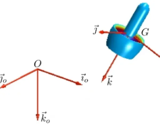
Figure 1: Attitude represents the orientation of body frameB = {G;⃗ı,⃗ȷ,⃗k} w.r.t. inertial frame I = {0;⃗ıo, ⃗ȷo, ⃗ko}.
that obtained from the accelerometer measurements. To cope with strong accelerations, a complementary GPS measurement of the vehicles linear velocity can be used to estimate its linear acceleration and, subsequently, to improve the precision of the attitude estimate [31], [15], [38]. In addition, in the case of an aircraft performing a level turn, air pressure sensors, such as pitot tubes that measure the magnitude of the airspeed, can be combined with accelerometer readings in order to derive a more precise estimate of the gravitational direction and, thus, significantly improve the quality of the attitude estimate [23].
The paper is organized as follows. In Section 2, attitude definition and parameterizations are recalled and discussed. In Section 3, existing attitude estimation methods based on vector observations, including both static and dynamics attitude estimation methodologies, are reviewed with a particular discussion on a nonlinear explicit complementary filter/observer [25] that was proposed by the last two authors of this paper and has become a common solution for most aerial robotic applications. Then, Section 4 presents some relevant nonlinear attitude observers for aerial robotic systems, that were developed on the basis of the explicit complementary filter. Finally, conclusions are given in Section 5.
2
Attitude parameterizations
The attitude represents the orientation of a frame, attached to the moving rigid body (i.e., body frame B), with respect to (w.r.t.) an inertial reference frameI (see Fig. 1). It can be described by a rotation matrix, an element of the special orthogonal group SO(3), where
SO(3), {R ∈ R3×3| det(R) = 1, RTR = RRT = I3}.
By denoting such a rotation matrix as R∈ SO(3), it satisfies the following differential equation ˙
R = RS(ω), (1)
where ω = [ω1, ω2, ω3]T ∈ R3is the angular velocity vector of the body frame relative to the inertial frame, expressed
in the body frame; and the notation S(·) denotes the skew-symmetric matrix associated with the cross product ×, i.e.,∀a, b ∈ R3, S(a)b = a× b.
Studies about the rotation group SO(3) started in the eighteenth century, and the problem of parameterization of the group of rotation of the Euclidean 3D-space has received great interest since 1776, when Euler showed that this group is a three-dimensional manifold. A rotation matrix has nine scalars components, but an element of the group of rotation can be represented by a set of less than nine parameters. Three is the minimum number of parameters required for this. However, it was shown that no three-dimensional parameterization can be 1-1 (i.e., its transformation to SO(3) is a global diffeomorphism) [45]. Previously, Hopf showed in 1940 that no four-dimensional parameterization can be 1-1, and that a five-dimensional parameterization can be used to represent the rotation group in a 1-1 global manner. However, the greatest inconvenience of Hopf’s five-dimensional parameterization concerns the nonlinearity of the associated differential equations [45]. On the other hand, four-dimensional param-eterizations [45], [39], like the quaternions parameterization, only represent the rotation group in a 2-1 manner.
Nevertheless, although the quaternion parameterization is not 1-1, no difficulty arises for practical purposes, be-cause the transformation of a unit quaternion to SO(3) is a local diffeomorphism everywhere. Hereafter, the Euler angles and the quaternion parameterizations are recalled and discussed.
2.1
Euler angles parametrization
Among many three-dimensional parameterizations [45], the Euler angles are most widely-used. Their definition depends on the problem to be solved and on the chosen systems of coordinates. A definition commonly used in the aerospace field is the Euler angles parameterization with three angles ϕ, θ and ψ corresponding to roll, pitch and yaw respectively [45], [34]. These Euler angles allow a rotation matrix R to be factorized into a product of three matrices of rotation about three axes of the body frame as follows:
R = CψSψ −Sψ 0Cψ 0 0 0 1 Cθ0 01 Sθ0 −Sθ 0 Cθ 10 Cϕ0 −Sϕ0 0 Sϕ Cϕ ,
where S and C denote the sin(·) and cos(·) operators. They can be computed from the rotation matrix R as ϕ = atan2(r3,2, r3,3) θ =−asin(r3,1) ψ = atan2(r2,1, r1,1)
where ri,j is the component of row i and column j of R. The Euler angles kinematics satisfy [45], [34]
˙ ϕ = ω1+ Sϕ T θ ω2+ Cϕ T θ ω3 ˙ θ = Cϕ ω2− Sϕ ω3 ˙ ψ = Sϕ Cθω2+ Cϕ Cθω3
where T denotes the tan(·) operator. If r3,1 = ±1, then θ = ∓π/2, but ϕ and ψ are no longer well-defined.
Therefore, the Euler angles constitute a parameterization of the rotation group, except at points corresponding to θ = ±π/2. Furthermore, when θ = ±π/2, ˙ϕ and ˙ψ are not well-defined either. The problem of singularities is a weakness of the Euler angles parameterization and, as a matter of fact, of all three-dimensional parameterization techniques.
2.2
Unit quaternion parametrization
CCompared to three-dimensional parameterizations, four-dimensional parameterizations allow singularities to be avoided. The earliest formulation of the four-dimensional parameterization, as pointed out in [39], was given by Euler in 1776. Earlier in 1775, he stated that in three dimensions, every rotation has an axis. This statement can be reformulated as follows (see e.g. [39], [37] for the proof)
Euler’s theorem: For any R∈ SO(3), there is a non-zero vector v ∈ R3 satisfying Rv = v.
This theorem implies that the attitude of a body can be specified in terms of a rotation by some angle about some fixed axis. It also indicates that any rotation matrix has an eigenvalue equal to one. A number of four-dimensional parameterizations can be found in the literature (see e.g. [39], [7]) such as the Euler parameters, the quaternion parameters, the Rodrigues parameters, and the Cayley-Klein parameters. Here, only the quaternion parameters are presented.
The quaternions were first proposed by Hamilton in 1843 [14] and further studied by Cayley and Klein. A unit quaternion has the form
q = s + iv1+ jv2+ kv3,
where s, v1, v2, v3 are real numbers satisfying s2+ v21+ v22+ v23 = 1, called constituents of the quaternion q, and
i, j, k are imaginary units that satisfy
In the literature, the unit quaternion q can be represented in a more concise way as q = (s, v)∈ R×R3, where s∈ R
is the real part of the quaternion q and v = [v1, v2, v3]T ∈ R3is its pure part or imaginary part. The quaternions are
not commutative, but associative, and they form a group known as the quaternion group where the unit element is
1, (1, 0) and the quaternion product ⋆ associated with this group is defined by
[ s v ] ⋆ [ ¯ s ¯ v ] = [ s¯s− vTv¯ s¯v + ¯sv + v× ¯v ] .
The transformed rotation matrix R is uniquely defined from the unit quaternion q, using Rodrigues’ rotation formula R = I3+ 2s S(v) + 2S(v)2.
On the other hand, converting a rotation matrix to a quaternion is less direct. In fact, there always exists at least one component of the unit quaternion q different from zero. Once this component is identified, the quaternion can be deduced. Note that only two values of the unit quaternion q correspond to the rotation matrix R and that they have opposed signs. For example, if tr(R)̸= −1, then
s =±1 2 √ 1 + tr(R), S(v) = R− R T 4s . Finally, the quaternion kinematics are given by
˙ q = 1 2q ⋆ [ 0 ω ] .
The quaternion parameterization involves four parameters (i.e., only one redundant parameter) and is free of singularities. The associated differential equation is linear in q. Furthermore, the structure of the quaternion group is, by itself, of great interest.
3
Overview on attitude estimation based on vector observations
3.1
Algebraic attitude determination
The attitude is often reconstructed from the observation of at least two non-collinear vectors. The first solution is the TRIAD algorithm, proposed by Black in 1964 [44], which algebraically computes the attitude matrix from the information in both the body frame and the inertial frame of two non-collinear unit vectors. More precisely, by denoting vI1, vB1, v2I, vB2 as the vectors of coordinates, expressed in the inertial frame and the body frame respectively, of two unitary Euclidean vectors ⃗v1and ⃗v2, one has vI1 = RvB1, vI2 = RvB2, and the TRIAD algorithm provides the
attitude matrix R as R = 3 ∑ i=1 sirTi = [ s1 s2 s3 ] [ r1 r2 r3 ]T ,
with two orthonormal triads s1= vI1, s2= vI1 × vI2 |vI 1 × vI2| , s3= s1× s2, r1= vB1, r2= v1B× vB2 |vB 1 × vB2| , r3= r1× r2.
Although this algorithm is simple to implement, the resulting estimated attitude matrix, in the presence of mea-surement noises, is not guaranteed to remain in the rotation group SO(3), and, thus, additional projection of the computed attitude into the group SO(3) is often required (using, for example, the Gram-Schmidt orthonormaliza-tion). Moreover, the TRIAD algorithm can only accommodate two vector observations, which may lead to difficulty in treating information when the observation of more than two vectors is available. For instance, in this case, the observation of which pair of vectors provides the best attitude estimate using the TRIAD algorithm may not be known a priori. Additionally, it does not take the relative reliability of the vector observations into account, even in the case of two vector observations. These drawbacks of the TRIAD algorithm disappear in optimal algorithms, which compute the best attitude estimate based on a cost function for which all vector observations are taken into
account simultaneously. Optimal algorithms are, however, computationally more expensive than the TRIAD algo-rithm. The first and also the best-known optimal attitude estimation problem is the least-square Wahba problem [52]. It consists in finding a rotation matrix bA∈ SO(3) which minimizes the cost function
J (A),1 2 n≥2 ∑ i=1 ki|viB− AviI| 2, (2)
where A corresponds to the transpose of the estimated attitude bR ∈ SO(3) (i.e., A = bRT); {vB
i} is a set of
measurements of n (≥ 2) unit vectors, expressed in the body frame; {viI} are the corresponding unit vectors, expressed in the inertial frame; and {ki} is a set of non-negative weights which can be designed based on the
reliability of the corresponding measurements. Wahba’s problem allows arbitrary weighting of vector observations. In [42], the author proposes the particular choice ki= σ−2i , the inverse variance of the measurement vBi, in order to
relate Wahba’s problem to Maximum Likelihood Estimation of the attitude based on an uncorrelated noise model [42]. In fact, the cost function J (A) defined by Eq. (2) can be rewritten as
J (A) = 1 2 n∑≥2 i=1 kitr ( (viB− AviI)(viB− AviI)T)= 1 2 n∑≥2 i=1 ki ( |vI i| 2+|vB i | 2)− tr(ABT),
with B,∑ni=1≥2kiviB(vIi)T. Therefore, the problem of finding a rotation matrix bA which minimizes J (A) is
equiv-alent to finding a rotation matrix bA which maximizes tr(ABT). The first solutions to Wahba’s problem, based on this observation, were proposed in 1966 by Farrell and Stuelpnagel [53] and by Wessner, Velman, Brock in the same paper1. However, these solutions, being computationally expensive, are not well suited to real-time applications. For instance, Farrell and Stuelpnagel’s method requires a polar decomposition of the matrix B into a product B = U P (with U an orthogonal matrix2 and P a symmetric and positive semidefinite matrix) and a diagonalization of P into P = W DWT 3 (with W a orthogonal matrix and D a diagonal matrix whose diagonal elements are arranged
in decreasing order, i.e., D = diag(d1, d2, d3) with d1≥ d2≥ d3). The optimal rotation matrix bA is then given by
b
A = U W diag(1, 1, det(U ))WT.
As for Wessner’s solution, which is a particular case of Farrell and Stuelpnagel’s solution, the optimal rotation matrix bA is calculated according to
b
A =(BT)−1(BTB)1/2.
For this solution, due to the inverse of BT, a minimum of three (non-collinear) vector observations must be available,
knowing that two non-collinear vectors are sufficient for attitude reconstruction using the TRIAD algorithm. In addition, the calculation of the square root of the matrix BTB also requires expensive computation. For example,
it is necessary to diagonalize BTB as BTB = W BDBWBT to obtain ( BTB)1/2= W BD 1/2 B W T B.
No solution to Wahba’s problem was able to replace the TRIAD algorithm in practice, until Davenport’s q-method [10] and the numerical technique QUEST (QUaternion ESTimator) [41] were proposed. By using the quaternion parameterization, Davenport transformed Wahba’s problem into the problem of finding the largest eigenvalue λmaxof the symmetric Davenport matrix K∈ R4×4 defined by
K, [ C− γI3 z z⊤ γ ] , with C, B + BT, γ, tr(B), z ,∑n≥2
i=1 kivBi × viI. The optimal quaternion, corresponding to the optimal rotation
matrix bA of Wahba’s problem, is the normalized eigenvector qmax of K associated with the eigenvalue λmax. In
fact, the largest eigenvalue λmax may be obtained by solving analytically the largest zero of the fourth-degree
characteristic polynomial det(K− λI4) [10]. However, Davenport’s q-method is also computationally complex. This
leads to the development of the QUEST algorithm by Shuster [41] on the basis of Davenport’s q-method. QUEST consists in solving numerically the equation det(K− λI4) = 0, or equivalently
λ4− (a + b)λ2− cλ + (ab + cγ − d) = 0, (3) with4a, γ2−tr(adj(C)), b , γ2+|z|2, c, det(C)+z⊤Cz, d, z⊤C2z. More precisely, based on Shuster’s observation
1These solutions were sent to Wahba and he presented them in that paper. 2det(U ) can be either 1 or−1.
3Note that any symmetric matrix is diagonalizable. 4Recall that adj(A) A = A adj(A) = det(A)I
that λmax is close to λo,
∑n≥2
i=1 ki, QUEST makes use of the Newton-Raphson method to solve Eq. (3), with
λo as the initial guess. It thus avoids the computation of all eigenvalues of K (i.e., all solutions to Eq. (3)).
QUEST is theoretically less robust than Davenport’s q-method, but it is clearly faster (normally few iterations are sufficient) and has proven to be reliable in practice (e.g., QUEST was implemented in the Magsat satellite in 1979). Many alternative numerical solutions for QUEST and Davenport’s q-method to Wahba’s problem have been proposed like, for instance, the Singular Value Decomposition (SVD), the Fast Optimal Attitude Matrix (FOAM), the Estimator of the Optimal Quaternion (ESOQ), ESOQ-1, ESOQ-2 algorithms [29]. These solutions, along with QUEST, for Wahba’s problem require a trade-off between computational time and precision; for instance, the number of iterations has to be defined in advance. Additionally, their main shortcoming concerns the memoryless characteristic in the sense that information contained in measurements of past attitudes is not preserved.
3.2
Dynamics attitude filtering and estimation
Since a filtering algorithm is usually preferred when measurements are obtained over a range of times and especially when vector measurements are noisy, many alternative solutions to algebraic methods have been proposed. They combine the vector measurements with the kinematic equation of rotation (i.e., Eq. (1)) and the angular velocity measurements. In this manner, the attitude estimation methods such as TRIAD, QUEST, SVD, FOAM, ESOQ, etc. can still be used as a preprocessor (i.e., the role of an attitude sensor) for a certain number of attitude filtering methods, such as in many Kalman filters (KFs), extended Kalman filters (EKFs), or Kalman-like filters (see, e.g., [11], [21], [28], [9], [3] and the references therein), or nonlinear observers (see, e.g., [40], [24], [25], [47], [51]). However, this process is not a prerequisite and is loosened in many attitude filtering methods, including KFs and EKFs, as proposed in [43], [1], [13], [25], [26], [30], [50], [9], etc. This leads to simpler, faster, and (probably) more accurate methodologies. For instance, consider the filter QUEST algorithm (a recursive discrete-time Kalman-like estimator) [43]. The author proposes to calculate the estimated attitude using QUEST algorithm and by propagating and updating the matrix B (which is, itself, involved in the Davenport matrix K) as
B(tk) = µΦ3×3(tk, tk−1)B(tk−1) + nk
∑
i=1
kiviB(vIi)T,
where Φ3×3(tk, tk−1)B(tk−1) is the state transition matrix of the transpose of the rotation matrix R, µ is a fading
memory factor and nk is the number of vector observations at time tk. An alternative sequential algorithm for the
filter QUEST is the recursive quaternion estimator (REQUEST) [1] which propagates and updates the Davenport matrix K by K(tk) = µΦ4×4(tk, tk−1)B(tk−1) + nk ∑ i=1 kiKi,
where Φ4×4(tk, tk−1)B(tk−1) is the quaternion state transition matrix and Ki is the Davenport matrix for a single
vector observation Ki= [ vBi(viI)T+vI i(vBi)T−((viB)TviI)I3 (viB× viI) (vBi × vIi)T (vB i )TviI ] .
The main shortcoming of the filter QUEST and REQUEST algorithms concerns the fading memory factor µ which, being arbitrarily chosen, makes these solutions suboptimal filters. This leads to the development of the Optimal-REQUEST algorithm [8][Ch.3] which, being essentially based on the Optimal-REQUEST algorithm, further optimally cal-culates the fading memory factor µ in the update stage of REQUEST according to a covariance optimization argument. Note that the filter QUEST, REQUEST, and Optimal-REQUEST algorithm, being based on QUEST, are numerical gradient methods and computationally more expensive than other modern algorithms (such as non-linear attitude observers) due to their optimization-based nature.
Other worthy examples are nonlinear attitude observers. The earliest nonlinear observer was proposed by Sal-cudean [40] using the unit quaternion representation. This work has led to the development of a significant body of nonlinear attitude observers over the last fifteen years, by exploiting either the unit quaternion or the rotation matrix [40], [35], [51], [47], [24], [46], [25], [49], [32], [12], [16]. The performance of recent observers is comparable to modern nonlinear filtering techniques [9]. They generally have much stronger stability and robustness properties and are simple to tune and implement [25]. Most early nonlinear attitude observers were developed on the basis of Lyapunov analysis. However, the attitude estimation problem has also become an intuitive example for the development of recent theories on invariant observers for systems with symmetry [4], [5], [6], [25], [19], [48]. For
instance, an illustrative example concerning the nonlinear explicit complementary filter proposed by Mahony et al. [25] is taken. This method is basically inspired by the Luenberger observer [22] in the sense that the dynamics of the estimated attitude bR contains two parts: a main part copying the dynamics of the real attitude (i.e., Eq. (1)) and an innovation part allowing the correction of the estimated attitude to the real attitude. For instance, if the gyro measurements are not affected by biases, the observer dynamics is given as
˙b R = bRS ( ω + n ∑ i=1 kiviB× bviB ) , (4)
with kipositive constant gains designed based on the reliability of the corresponding measurements, andbviB, bRTvIi.
An important issue of the attitude filtering concerns the gyro bias, leading to a complementary approach in which the gyroscopes are used to filter the vector measurements, which are in turn used to estimate the gyro bias (e.g., [25], [47], [51]). By making a constant gyro bias assumption (i.e., ωy = ω + bω, with ωy the gyro measurement and bω
the constant gyro bias vector), a complete version of the explicit complementary filter is given as [25] ˙b R = RS(ωb y− bbω+ σR) ˙bbω = σb σR , n ∑ i=1 kiviB× bviB σb , −kbσR (5)
with kb, ki positive constants. This is a continuous version; however, a discrete version can be easily derived. It
can also be conveniently rewritten in quaternion form [25], [16]. Furthermore, a fast attitude estimation method from vector observations like TRIAD or QUEST can be used for a good initial attitude estimate. This observer is derived by considering the Lyapunov function candidate
L , n ∑ i=1 ki|viB− bR TvI i| 2+ 2 kb |bω− bbω|2 (6)
whose derivative along any solution to the error system is ˙L = −2∥Pa( eRM )∥2 ≤ 0, with eR , bRTR, M ,
∑n
i=1viB(vBi)
T,∥ · ∥ the Frobenius norm and P
a(·) the skew-symmetric projection operator in square matrix space.
With at least two non-collinear vector observations the estimated attitude asymptotically converges to the real one, for almost all initial conditions, even in the case of time-varying vectors (see [25], [48] for the detailed proofs). This is the strongest possible result knowing that no smooth globally asymptotically stable observers exist on SO(3) due to the topology obstruction of the rotation group [2]. In the case of a single vector observation, the solutions to this filter are still well-posed, whereas analytically reconstructing the attitude from a single vector observation is not possible. In particular, almost-global asymptotical stability is still ensured in the case of a single vector observation under the persistent excitation assumption (i.e., if the vector’s direction or the vehicle’s attitude is permanently varying) [26].
Remark 1 Interestingly, the first term in the right-hand side of the Lyapunov functionL defined by (6) corresponds
to the cost function J ( bRT) related to Wahba’s problem. Therefore, in the absence of gyro bias, the (numerical)
solution to the bias-free explicit complementary filter (4) converges asymptotically/exponentially to the optimal solution to Wahba’s problem for almost all initial conditions under observability conditions.
A generalized version of the explicit complementary filter (5) recently proposed by Jensen [18] is given as follows ˙b R = RS(ωb y− bbω+ KPσ) ˙bbω = −KIσ σ , n ∑ i=1 kivBi × bvBi (7)
with ki positive constant scalar gains; KP and KI symmetric positive definite matrices (not necessarily
con-stant). Clearly, this generalized observer offers a larger tuning space than the explicit complementary filter (5) while ensuring similar stability and convergence properties; and it is shown that bias-free multiplicative extended Kalman filter (MEKF) and constant-gain MEKF correspond to its particular cases [18].
4
Nonlinear attitude observers for aerial robotic systems
4.1
Sensor measurements
The most basic instrumentation embarked on an aerial robot for attitude estimation is a MEMS IMU, which can be complemented with a GPS or airspeed sensors. Assume that the IMU consists of a 3-axis gyroscope, a 3-axis accelerometer and a 3-axis magnetometer.
• The 3-axis gyroscope measures the angular velocity ω
ωy= ω + bω+ ηω,
where ηω∈ R3 is the measurement noise and bω∈ R3 denotes a constant (or slowly time-varying) gyro bias.
Generally, gyroscopes are rather robust to noise and quite reliable for aerial robotics applications.
• The specific acceleration aB∈ R3 expressed in the body-fixed frameB is defined as aB= RT( ˙v− ge3), where
the vehicle’s acceleration expressed in the inertial frame I is ˙v, and the gravitational acceleration expressed in the frameI is ge3, with e3= (0, 0, 1)T. The 3-axis accelerometer measures this specific acceleration
ay = aB+ ba+ ηa,
where ηa∈ R3is the measurement noise and bω∈ R3denotes a bias term. Accelerometers are highly sensitive
to vibration and, thus, often require significant low-pass mechanical and/or digital filtering to be usable. • The 3-axis magnetometer measures the ambient magnetic field
my= mB+ Bm+ ηm,
where ηm ∈ R3 is the measurement noise, mB = RTmI ∈ R3 is the Earth’s magnetic field expressed in the
body frameB and Bm∈ R3 represents the sum of all local magnetic disturbances generated by motors and
currents, as well as external magnetic fields experienced by vehicles that manoeuvre in built environments. While the magnetometer noise ηm is usually low, the local magnetic disturbance Bm can be significant,
especially if the sensor is near the power wires of the motors.
4.2
Application of the explicit complementary filter for IMUs
In view of the attitude estimation survey in Section 3, most existing methods of attitude estimation make use of the measurement of at least two known non-collinear inertial vectors. Obtaining measurements of two known vectors is, however, difficult in practice and in particular for small aerial robots. In fact, while the magnetometer provides a vector measurement related to the Earth’s magnetic field, the accelerometer does not directly measure the gravitational direction. This is due to the vehicle’s linear acceleration involved in the specific acceleration that is measured by the accelerometer. However, most robotic vertical take-off and landing (VTOL) vehicles (such as multicopters, or ducted fans) spend a significant amount of time in near hovering or slow forward flight, with ˙v≈ 0; thus, using the accelerometer as an inclinometer has been shown to be efficient in practice during this flight regime. In fact, it is known that for an ideal thrust controlled aerial vehicle, the measurement of the gravitational direction cannot be directly extracted from accelerometer measurement data [27], [33], [36]. However, VTOL robotic vehicles are subject to secondary aerodynamic forces (e.g., blade flapping and induced drag) that inject low frequency information on the gravitational direction into the accelerometer measurements [27], [33]. It follows that the model aB ≈ −gRTe3is an effective model for vector attitude measurement in a wide range of practical systems [13], [24],
[25], [32].
4.2.1 Standard implementation and associated coupling issues
Once the approximation aB ≈ −gRTe3 is made, the standard implementation of the explicit complementary filter
(5) consists in defining the innovation term σRas [25]
σR, k1uB× buB+ k2m¯B× b¯mB, (8)
with k1,2 positive constant gains, uB , −aB/g, uI , e3, buB , bRTuI, ¯mB , mB/|mI|, ¯mI , mI/|mI|, b¯mB ,
b RTm¯
I. However, it has been recognized that this standard implementation encounters some coupling issues that
• Magnetic disturbances and bias influence the estimation of roll and pitch angles. In many applications espe-cially for small-size electric motorized aerial robots, significant magnetic disturbances are almost unavoidable, leading to significant time-varying deterministic error between mB and RTm
I. This not only leads to large
estimation errors of the yaw angle but also non-negligible errors in the roll and pitch estimation.
• The dynamics of roll, pitch and yaw estimates are highly coupled. This implies that the estimation of the yaw angle strongly affects the estimation of the roll and pitch angles. This issue can be observed by analyzing the linearized system around the system equilibrium. For the sake of simplicity, let us, for instance, neglect the gyro-bias bωand the dynamics of the estimated bias bbωonly in this discussion. This supposition in association
with Eqs. (5) and (8) yields the following dynamics of the error attitude matrix eR = R bRT
˙e
R =−(k1e3× eRe3+ k2m¯I× eR ¯mI)×R.e (9)
Consider a first order approximation of eR around the equilibrium eR = I3as eR≈ I3+ x×, with x∈ R3. Note
that locally the first, second and third components of x correspond, respectively, to the roll, pitch and yaw error estimates. From Eq. (9) it can easily be verified that
˙ x≈
−k1−k2(1− ¯m
2
I,1) k2m¯I,1m¯I,2 k2m¯I,1m¯I,3
k2m¯I,1m¯I,2 −k1−k2(1− ¯m2I,2) k2m¯I,2m¯I,3
k2m¯I,1m¯I,3 k2m¯I,2m¯I,3 −k2(1− ¯m2I,3)
x (10)
In practice, the gravity vector and the Earth’s magnetic field vector (i.e., e3and ¯mI) can be “ill-conditioned”
in the sense that they are very close to each other. In such a case, the third component of ¯mI is dominant to its first and second ones. For example, in France ¯mI,3≈ 0.9. As a consequence, in view of Eq. (10) the dynamics of the roll and pitch errors (i.e., x1and x2) are strongly coupled with the yaw error dynamics (i.e.,
x3).
• On the other hand, the ill-conditioning of the two vectors e3 and ¯mI may also lead to the impossibility of
finding a set of “non-high” gains {k1, k2} so as to provide the system with fast time response, bearing in
mind that high gains may excessively amplify measurement noises. For discussion purposes and without loss of generality, let us, for instance, assume that ¯mI,2≈ 0 (i.e., ¯m2
I,1+ ¯m2I,3≈ 1) and ¯m2I,3≫ ¯m2I,1. Under this
approximation, it is straightforward to verify that three poles of System (10) are given by: λ1=−(k1+k2) λ2=−12(k1+k2) ( 1+ √ 1−4k1k2m¯ 2 I,1 (k1+k2)2 ) λ3=−12(k1+k2) ( 1− √ 1−4k1k2m¯ 2 I,1 (k1+k2)2 ) ≈−k1k2m¯2I,1 k1+k2
The pole λ1 is associated with the pitch dynamics, and the poles λ2 and λ3 are associated with the coupled
roll and yaw dynamics. The less negative pole λ3, approximated by−k1k2m¯2I,1/(k1+k2), will be very close
to zero if k1and k2 are not chosen sufficiently high, since ¯m2I,1≪ 1. This leads to slow time response of the
coupled roll and yaw dynamics.
4.2.2 Modified solutions for overcoming coupling issues
Decoupling of input signals to ensure that the roll and pitch estimates are not influenced by magnetic disturbances was considered in [32], [30], [17], [16] and represents an important modification of the standard implementation of the explicit complementary filter (i.e., Observer (5) with σR given by (8)) in order to improve the overall quality
of the attitude estimate. Let us discuss these strategies.
The solution proposed by Martin and Salaun [30], [32] consists in creating another inertial vector as the cross product of the gravitational direction and the Earth’s magnetic field direction, and its associated “artificial” mea-surement based on the cross product of accelerometer and magnetometer meamea-surements. More precisely, the following vectors are computed
vI , uI× mI
|uI× mI|, vB,
uB× mB
with uB, −aB/g, uI , e3. Then, the explicit complementary filter (5) can be applied with the innovation term
σR now defined as (compare to (8))
σR, k1uB× buB+ k2vB× bvB, (12)
with k1,2 positive constant gains, buB , bRTuI, bvB , bRTvI. This solution ensures the decoupling of the roll and
pitch estimates from magnetic disturbances locally in the general case [30] and globally in the presence of a constant magnetic bias in the inertial frame (as additionally proved in [17]).
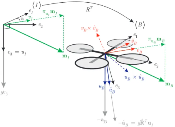
Inspired by the work of Martin and Salaun, we have proposed another observer termed conditioned observer [16], which still takes the same form as the explicit complementary filter (5) but with the modified innovation terms σR and σb given by { σR, k1uB× buB+ k2 ( (vB× bvB)TbuB)buB σb, k3uB× buB+ k4vB× bvB (13)
with k1,2,3,4 positive constant gains satisfying k3> k4, uB, −aB/g, uI , e3, and (compare to (11) and see Fig. 2)
vI, πuImI |πuImI|
, vB, πuBmB |πuImI|
, (14)
with πx, |x|2I3− xxT,∀x ∈ R3, denoting the projection on the plan orthogonal to x. The conditioned observer
ensures the global decoupling of the roll and pitch estimates from magnetic disturbances and also from the dynamics of yaw estimate in the general case. This decoupling property is clearly stronger than that of the previous solution. Moreover, in contrast with the standard implementation of the explicit complementary filter (5), fast convergence rate can still be achieved with non-high gains even in the case of ill-conditioning of the gravity and Earth’s magnetic field directions [16].
Figure 2: Vectors involved in the conditioned observer.
4.3
GPS-aided attitude observers
Most existing (“classical”) attitude observers/filters rely on the small acceleration assumption (i.e., ˙v≪ g) so that the gravitational direction measurement can be approximated by the accelerometer measurement, as discussed in the previous subsection. For many VTOL vehicles in aggressive motion, however, the vehicle’s linear accelerations can be important and can induce large errors on the attitude estimate. This is also the case for fixed-wing aircraft manoeuvring in a limited space and making some rapid turns. To deal with strong linear accelerations, a comple-mentary GPS measurement of the linear velocity can be combined with the accelerometer measurement to estimate the vehicle’s acceleration and, subsequently, improve the precision of the attitude estimate. In this way, some GPS–aided attitude observers have been proposed recently [31], [15], [38] on the basis of the following differential
equations {
˙v = ge3+ RaB
˙
For instance, the cascade attitude observer proposed by Hua [15] consists in, first, estimating the specific acceleration expressed in the inertial frame aI , ˙v − ge3 and, then, in using this estimated value along with magnetometer
measurements to recover the whole attitude estimate on the basis of the explicit complementary filter [25]. More precisely, in order to estimate the specific acceleration aI, the following observer was proposed
{ ˙bv = k1(v− bv) + ge3+ QaB ˙ Q = QS(ω) + kv(v− bv)aBT − kqmax(0,∥Q∥ − √ 3)Q (16)
with k1, kv, kq positive constant gains and Q∈ R3×3 an auxiliary matrix which is not a rotation matrix. The last
term in the expression of ˙Q creates a dissipative effect when the Frobenius norm of Q becomes larger than √3, allowing it to be driven back to this threshold and thus avoiding numerical drifts of Q. It is shown that the errors (aI− QaB, v− bv) converge to zero [15]. Consequently, one can view either QaB or QaB+ k1(v− bv) as the estimate
of aI. From here, the author proposed the following attitude observer on the basis of the explicit complementary filter [25] {
˙b
R = RS(ω + σb R)
σR , k2mB× bRTmI+ k3aB× bRT(QaB+ k1(v− bv))
(17) with k2,3 positive constant gains. Almost global convergence of the observer is proved. Furthermore, in the special
case of constant accelerations of the vehicle, almost-global asymptotic stability of the observer is achieved.
Invariant attitude observers: When the objective consists in combining the estimation of the attitude and the
filtering of the linear velocity (and eventually the position), some invariant attitude observers have been proposed recently [31], [15], [38]. The earliest nonlinear invariant GPS–aided attitude observer was proposed by Martin and Salaun [31]. When measurements are not affected by bias, this observer has the form
˙bv = k1(v− bv) + ge3+ bRaB ˙b R = RS(ω + σb R) σR , k2((mB× bRTmI)TaB)aB+ k3aB× bRT(v− bv) (18)
with k1,2,3 positive constant gains. This defines an invariant observer [5], [20] in the sense that it preserves the
(Lie group) invariance properties of System (15) w.r.t. constant velocity translation v 7→ v + v0 and constant
rotation of the body frame R 7→ RR0. A practical advantage of this solution is the (local) decoupling of the roll
and pitch angles estimation from the measurements of the Earth’s magnetic field (which may be rather erroneous due to magnetic disturbances). However, only local exponential stability of the estimation error is proven in [31] (based on the linearized estimation error dynamics), under some assumptions on the reference motion (i.e., “smooth trajectory”).
Motivated by this result, other GPS-aided attitude invariant observers have been proposed with associated Lyapunov-based convergence and stability analyses [15], [38]. The invariant observer proposed by Hua [15] is given
by ˙bv = k1(v− bv) + ge3+ bRaB ˙b R = RS(ω + σb R) σR , k2mB× bRTmI+ k3aB× bRT(v− bv) (19)
with k1,2,3positive constant gains. In fact, observer (19) is slightly different from observer (18), which is a simplified
version of the observer proposed in [31] suited to the case without gyro biases. The sole difference between observers (18) and (19) lies in the definition of σR where the term k2((mB× bRTmI)TaB)aB in (18) is replaced in (19) by
k2(mB× bRTmI). Another invariant observer was proposed by Robert and Tayebi [38], which can be rewritten in
the following form ˙bv = k1(v− bv) + ge3+ bRaB+ 1 k1 b RS(σR)aB ˙b R = RS(ω + σb R) σR , k2mB× bRTmI+ k3aB× bRT(v− bv) (20)
with k1,2,3 positive constant gains. The additional term (1/k1) bRS(σR)aB involved in the dynamics of bv in (20)
constitutes the difference between observers (20) and (19), allowing the authors to establish simpler Lyapunov-based stability and convergence analyses. The main interest of both studies [15] and [38] is to yield semi-global
exponential convergence proofs. Both observers (19) and (20) guarantee the semi-global stability property under a “high-gain”-like condition on k1which indicates that the size of basin of attraction is proportional to k1 and tends
to be almost-global when k1 tends to infinity. In fact, the “high-gain” condition is only sufficient, and simulation
results seem to indicate that the basin of attraction does not depend on the value of k1(> 0). But the proof of this
property remains an open problem.
It is worth noting that, contrary to observer (18), all three observers (19), (20) and (16)–(17) do not ensure the (local) decoupling of the estimation of the roll and pitch (Euler) angles from the magnetic measurements. This suggests –as an open problem– the design of an observer that combines the advantages of these observers. For instance, observers (18) and (16)–(17) can be combined, yielding the following attitude observer (in the replacement of (17)) {
˙b
R = RS(ω + σb R)
σR , k2((mB× bRTmI)TaB)aB+ k3aB× bRT(QaB+ k1(v− bv))
(21)
with Q the (numerical) solution to System (16). Specifying the stability domain of this observer, however, remains open.
4.4
Airspeed-aided attitude observer for fixed-wing UAVs
For fixed-wing UAVs that manoeuvre in GPS denied environments (e.g., indoor or near to buildings), an alternative solution of attitude estimation based on IMU and improved with GPS data is the use of pressure sensors such as pitot tubes that measure the magnitude of the airspeed (i.e., the speed of the vehicle relative to the air) as a replacement of GPS velocity measurements. A nonlinear complementary filter/observer of this nature was proposed [23]. Magnetometer is not used in this study since the authors are only interested in roll and pitch estimation, but the incorporation of magnetometer measurements into the observer for additional yaw estimation can be done as described hereafter.
In [23], Mahony et al. consider the case where an aircraft performs a level turn (i.e., constant altitude) with constant turn radius ρ > 0 and zero sideslip angle. In this case, the vehicle experiences the centripetal acceleration
ac≈ ω × (ω × ρr),
with r the unit vector from the aircraft to the turning center. In order to eliminate the dependence on the unknown turn geometry, the approximation ω× ρr ≈ Vairis made, so that the centripetal acceleration can be approximately
given by ac ≈ ω × Vair. The airspeed vector Vair is not directly measured, but it can be recovered from the
measurement of the norm |Vair| given by the pitot tubes and from the knowledge of the angle-of-attack α as follows
Vair=|Vair| Cα0 Sα . (22)
The linearized dynamics model of the angle-of-attack approximately satisfy ˙
α =− c0 |Vair|
α + ˙θ + α0, (23)
with c0 and α0 constant parameters, and ˙θ≈ ω2. By numerically integrating Eq. (23), the angle-of-attack α can
be obtained, which enables the computation of the airspeed vector Vairaccording to Eq. (22) and, subsequently, of
the approximated measurement of the centripetal acceleration ac (≈ ω × Vair).
Once the centripetal acceleration ac is computed, the gravitational direction expressed in the body frame can
also be obtained from accelerometer readings as
uB= RTuI ≈−(aB− ac) |aB− ac|
,
with uI, e3. Then, the explicit complementary filter (5) can be applied with the innovation term σR defined as
with positive constant gain k1 andbuB , bRTuI. Although, several assumptions and approximations are made, the
reported experimental results are quite satisfactory [23].
The yaw angle may be recovered under the persistent excitation condition [26]. It can also be estimated when magnetometer measurements are involved by using the conditioned observer [16] (i.e., observer (5) with the innovation terms σR and σb defined by (13)–(14)).
5
Conclusions
Several attitude estimation techniques –ranging from algebraic vector observations-based attitude determination algorithms to dynamics attitude filtering and estimation methodologies– have been reviewed and commented upon in relation to practical implementation issues. A particular attention is devoted to the applications of the well-known nonlinear explicit complementary filter/observer [25] to aerial robotics, using a low-cost and light-weight inertial measurement unit, which can be complemented with a GPS or airspeed sensors. In the case of “weak” linear accelerations, the vector direction estimate of the gravitational direction can be derived from accelerometer measurements with reasonably good accuracy and, thus, the explicit complementary filter can be directly applied. In this case, decoupling of input signals to ensure that the roll and pitch estimates are not disturbed by deviation in the magnetometer measurements represents an important improvement of the basic algorithm. On the other hand, in the case of “strong” linear accelerations, the combination of IMU with GPS-velocity or airspeed measurements allows the overall quality of the attitude estimate to be effectively improved.
Acknowledgments
This work has been supported by the French Agence Nationale de la Recherche through the ANR ASTRID SCAR project “Sensory Control of Aerial Robots”.
Acronyms
• IMU: Inertial Measurement Unit. • GPS: Global Positioning System. • MEMS: microelectromechanical systems. • VTOL: vertical take-off and landing. • UAV: Unmanned Aerial Vehicle. • QUEST: QUaternion ESTimator. • SVD: Singular Value Decomposition. • FOAM: Fast Optimal Attitude Matrix. • ESOQ: Estimator of the Optimal Quaternion.
References
[1] I. Y. Bar-Itzhack. REQUEST: a recursive QUEST algorithm for sequentiel attitude determination. AIAA Journal of Guidance, Control, and Dynamics, 19(5):1034–1038, 1996.
[2] S. P. Bhat and D. S. Bernstein. A topological obstruction to continuous global stabilization of rotational motion and the unwinding phenomenon. Systems & Control Letters, 39(1):63–70, 2000.
[3] S. Bonnabel. Left-invariant extended Kalman filter and attitude estimation. In IEEE Conf. on Decision and Control, pages 1027–1032, 2007.
[4] S. Bonnabel, P. Martin, and P. Rouchon. Groupe de Lie et observateur non-lin´eaire. In Conf´erence Interna-tionale Francophone d’Automatique 2006, 2006.
[5] S. Bonnabel, P. Martin, and P. Rouchon. Symmetry-preserving observers. IEEE Trans. on Automatic Control, 53(11):2514–2526, 2008.
[6] S. Bonnabel, P. Martin, and P. Rouchon. Non-linear symmetry preserving observers on lie groups. IEEE Trans. on Automatic Control, 54(7):1709–1713, 2009.
[7] M. Le Borgne. Quaternions et controle sur l’espace de rotation. Technical Report 751, INRIA, 1987.
[8] D. Choukroun. Novel methods for attitude determination using vector observations. PhD thesis, Israel Institute of Technology, 2003.
[9] J. L. Crassidis, F. L. Markley, and Y. Cheng. Survey of nonlinear attitude estimation methods. AIAA Journal of Guidance, Control, and Dynamics, 30(1):12–28, 2007.
[10] P. B. Davenport. A vector approach to the algebra of rotations with applications. Technical Report TN D-4696, NASA, 1968.
[11] J. L. Farrell. Attitude determination by Kalman filtering: Volume I. Technical Report CR598, NASA, 1964. [12] H. F. Grip, T. I. Fossen, T. A. Johansen, and A. Saberi. Attitude estimation using biased gyro and vector
measurements with time-varying reference vectors. IEEE Trans. on Automatic Control, 57(5):1332–1338, 2012. [13] T. Hamel and R. Mahony. Attitude estimation on SO(3) based on direct inertial measurements. In IEEE Conf.
on Robotics and Automation, pages 2170–2175, 2006.
[14] W. R. Hamilton. Letter from Sir William R. Hamilton to John T. Graves, Esq. on Quaternions, 1843. [15] M.-D. Hua. Attitude estimation for accelerated vehicles using GPS/INS measurements. Control Engineering
Practice, 18(7):723–732, 2010.
[16] M.-D. Hua, G. Ducard, T. Hamel, R. Mahony, and K. Rudin. Implementation of a nonlinear atti-tude estimator for aerial robotic vehicles. IEEE Trans. on Control Systems Technology, 2013. DOI: 10.1109/TCST.2013.2251635.
[17] M.-D. Hua, K. Rudin, G. Ducard, T. Hamel, and R. Mahony. Nonlinear attitude estimation with measurement decoupling and anti-windup gyro-bias compensation. In IFAC World Congress, pages 2972–2978, 2011. [18] K. J. Jensen. Generalized nonlinear complementary attitude filter. AIAA Journal of Guidance, Control, and
Dynamics, 34(5):1588–1592, 2011.
[19] C. Lageman, J. Trumpf, and R. Mahony. Gradient-like observers for invariant dynamics on a Lie group. IEEE Trans. on Automatic Control, 55(2):367–377, 2010.
[20] C. Lageman, J. Trumpf, and R. Mahony. Gradient-like observers for invariant dynamics on a Lie group. IEEE Trans. on Automatic Control, 55(2):367–377, 2010.
[21] E. Lefferts, F. Markley, and M. Shuster. Kalman filtering for spacecraft attitude estimation. AIAA Journal of Guidance, Control, Navigation, 5:417–429, 1982.
[22] D. Luenberger. An introduction to observers. IEEE Trans. on Automatic Control, 16(6):596–602, 1971. [23] R. Mahony, M. Euston, J. Kin, P. Coote, and T. Hamel. A non-linear observer for attitude estimation of a
fixed-wing Unmanned Aerial Vehicle without GPS measurements. Transactions of the Institute of Measurement and Control, 33(6):699–717, 2011.
[24] R. Mahony, T. Hamel, and J.-M. Pflimlin. Complementary filter design on the special orthogonal group SO(3). In IEEE Conf. on Decision and Control, pages 1477–1484, 2005.
[25] R. Mahony, T. Hamel, and J.-M. Pflimlin. Nonlinear complementary filters on the special orthogonal group. IEEE Trans. on Automatic Control, 53(5):1203–1218, 2008.
[26] R. Mahony, T. Hamel, J. Trumpf, and C. Lageman. Nonlinear attitude observers on SO(3) for complementary and compatible measurements: A theoretical study. In IEEE Conf. on Decision and Control, pages 6407–6412, 2009.
[27] R. Mahony, V. Kumar, and P. Corke. Multirotor Aerial Vehicles: Modeling, Estimation, and Control of Quadrotor. IEEE Robotics & Automation Magazine, 19(3):20–32, 2012.
[28] F. L. Markley. Attitude error representations for Kalman filtering. AIAA Journal of Guidance, Control, and Dynamics, 26(2):311–317, 2003.
[29] F. L. Markley and D. Mortari. Quaternion attitude estimation using vector observations. The Journal of the Astronautical Sciences, 48(2, 3):359–380, 2000.
[30] P. Martin and E. Salaun. Invariant observers for attitude and heading estimation from low-cost inertial and magnetic sensors. In IEEE Conf. on Decision and Control, pages 1039–1045, 2007.
[31] P. Martin and E. Salaun. An invariant observer for Earth-Velocity-Aided attitude heading reference systems. In IFAC World Congress, pages 9857–9864, 2008.
[32] P. Martin and E. Salaun. Design and implementation of a low-cost observer-based attitude and heading reference system. 18(7):712–722, 2010.
[33] P. Martin and E. Salaun. The true role of Accelerometer Feedback in Quadrotor Control. In IEEE Conf. on Robotics and Automation, pages 1623–1629, 2010.
[34] A. Mayer. Rotations and their algebra. SIAM Journal on Control and Optimization, 2(2):77–122, 1960. [35] H. Nijmeijer and T. I. Fossen. New Directions in Nonlinear Observer Design, volume 244 of Lecture Notes in
Control and Information Sciences. Springer, 1999.
[36] S. Omari, M.-D. Hua, G. Ducard, and T. Hamel. Nonlinear Control of VTOL UAVs Incorporating Flapping Dynamics. In International Conference on Intelligent Robots and Systems (IROS), pages ?–?, 2013.
[37] B. Palais and R. Palais. Euler’s fixed point theorem: The axis of a rotation. Journal of Fixed Point Theory and Applications, 2:215–220, 2007.
[38] A. Roberts and A. Tayebi. On the attitude estimation of accelerating rigid-bodies using GPS and IMU measurements. In IEEE Conf. on Decision and Control, pages 8088–8093, 2011.
[39] A. C. Robinson. On the use of quaternions in simulations of rigid-body motion. Technical Report 58-17, Wright Air Development Center, 1958.
[40] S. Salcudean. A globally convergent angular velocity observer for rigid body motion. IEEE Trans. on Automatic Control, 36(12):1493–1497, 1991.
[41] M. D. Shuster. Approximate algorithms for fast optimal attitude computation. In AIAA Guidance and Control Conference, pages 88–95, 1978.
[42] M. D. Shuster. Maximum likelihood estimation of spacecraft attitude. The Journal of the Astronautical Sciences, 37(1):79–88, 1989.
[43] M. D. Shuster. Kalman filtering of spacecraft attitude and the QUEST model. The Journal of the Astronautical Sciences, 38(3):377–393, 1990.
[44] M. D. Shuster. The QUEST for better attitudes. The Journal of the Astronautical Sciences, 54(3,4):657–683, 2006.
[45] J. Stuelpnagel. On the parametrization of the three-dimensional rotation group. SIAM Journal on Control and Optimization, 6(4):422–430, 1964.
[46] A. Tayebi, S. McGilvray, A. Roberts, and M. Moallem. Attitude estimation and stabilization of a rigid body using low-cost sensors. In IEEE Conf. on Decision and Control, pages 6424–6429, 2007.
[47] J. Thienel and R. M. Sanner. A coupled nonlinear spacecraft attitude controller and observer with an unknown constant gyro bias and gyro noise. IEEE Trans. on Automatic Control, 48(11):2011–2015, 2003.
[48] J. Trumpf, R. Mahony, T. Hamel, and C. Lageman. Analysis of non-linear attitude observers for time-varying reference measurements. IEEE Trans. on Automatic Control, 57:2789–2800, 2012.
[49] J. F. Vasconcelos, R. Cunha, C. Silvestre, and P. Oliveira. A landmark based nonlinear observer for attitude and position estimation with bias compensation. In IFAC World Congress, pages 3446–3451, 2008.
[50] J. F. Vasconcelos, C. Silvestre, and P. Oliveira. A nonlinear GPS/IMU based observer for rigid body attitude and position estimation. In IEEE Conf. on Decision and Control, pages 1255–1260, 2008.
[51] B. Vik and T. Fossen. A nonlinear observer for GPS and INS integration. In IEEE Conf. on Decision and Control, pages 2956–2961, 2001.
[52] G. Wahba. A least squares estimate of satellite attitude, Problem 65-1. SIAM Review, 7(3):409, 1965. [53] G. Wahba. A least squares estimate of satellite attitude. SIAM Review, 8(3):384–386, 1966.
Minh-Duc Hua graduated from Ecole Polytechnique, France, in 2006, and received his Ph.D. from the University
of Nice-Sophia Antipolis, France, in 2009. He spent two years as a postdoctoral researcher at I3S UNS-CNRS, France. He is currently researcher of the French National Centre for Scientific Research (CNRS) at the ISIR laboratory of the University Pierre and Marie Curie (UPMC), France. His research interests include nonlinear control theory, estimation and teleoperation with applications to autonomous mobile robots such as UAVs and AUVs.
Guillaume Ducard received his Master degree in Electrical Engineering from ETH Zurich in 2004. He completed
his doctoral work in 2007 and his two-year post doc in 2009 both at the ETH Zurich in the field of unmanned aerial vehicles. He is currently researching at I3S UNS-CNRS Sophia Antipolis, France, in nonlinear control and estimation, fault-tolerant flight control and guidance systems for UAVs, and formation flight control.
Tarek Hamel is Professor at the University of Nice Sophia Antipolis since 2003. He conducted his Ph.D. research
at the University of Technologie of Compi`egne (UTC), France, and received his doctorate degree in Robotics from the UTC in 1996. After two years as a research assistant at the (UTC), he joined the Centre d’Etudes de M´ecanique d’Ile de France in 1997 as an associate professor. His research interests include nonlinear control theory, estimation and vision-based control with applications to Unmanned Aerial Vehicles. He is currently Associate Editor for IEEE Transactions on Robotics and for Control Engineering Practice.
Robert Mahony received the B.Sc. degree in applied mathematics and geology and the Ph.D. degree in systems
engineering from the Australian National University (ANU), Canberra, in 1989 and 1995, respectively. He is currently a Professor in the Department of Engineering, ANU. He worked as a Marine Seismic Geophysicist and an Industrial Research Scientist before completing a Postdoctoral Fellowship in France and a Logan Fellowship at Monash University, Victoria, Australia. He has held his post at ANU since 2001. His research interests are in non-linear control theory with applications in robotics, geometric optimization techniques, and systems theory.