HAL Id: hal-01322698
https://hal.inria.fr/hal-01322698v2
Submitted on 18 Nov 2016
HAL is a multi-disciplinary open access
archive for the deposit and dissemination of sci-entific research documents, whether they are pub-lished or not. The documents may come from teaching and research institutions in France or abroad, or from public or private research centers.
L’archive ouverte pluridisciplinaire HAL, est destinée au dépôt et à la diffusion de documents scientifiques de niveau recherche, publiés ou non, émanant des établissements d’enseignement et de recherche français ou étrangers, des laboratoires publics ou privés.
Pricing European options and risk measurement under
exponential Lévy models - a practical guide
Khaled Salhi
To cite this version:
Khaled Salhi. Pricing European options and risk measurement under exponential Lévy models -a pr-actic-al guide. Intern-ation-al Journ-al of Fin-anci-al Engineering, World Scientific, 2017, 2 (2-3), 1750016 (36 p.). �10.1142/S2424786317500165�. �hal-01322698v2�
Pricing European options and risk measurement
under Exponential Lévy models - a practical guide
Khaled Salhi
a,b,c,†November 18, 2016
Abstract
This paper provides a thorough survey of the European option pricing, with new trends in the risk measurement, under exponential Lévy models. We develop all steps of pricing from equivalent martingale measures construction to numerical valuation of the option price under these measures. We then construct an algorithm, based on Rockafellar and Uryasev representation and fast Fourier transform, to compute Risk indicators, like the VaR and the CVaR of derivatives. The results are illustrated with an example of each exponential Lévy class. The main contribution of this paper is to build a comprehensive study from the theoretical point of view to practical numerical illustration and to give a complete characterization of the studied equivalent martingale measures by discussing their similarity and their applicability in practice. Furthermore, this work proposes applications to the Fourier inversion technique in risk measurement.
Keywords: Lévy process, incomplete market, Esscher martingale measure, minimal en-tropy martingale measure, fast Fourier transform, Risk, Conditional Value-at-Risk, Merton model, variance gamma model.
1
Introduction
Stochastic processes are intensively used for modeling financial markets. The Black and Scholes model is one of the most known models. It describes the stock price as a geometric Brownian motion. In this context, the option pricing problem is solved using the risk neutral approach [8]. The key tool is the uniqueness of the equivalent martingale measure (EMM) and the derivative price is therefore the unique arbitrage-free contingent claim value.
It has become clear, however, that this option pricing model is inconsistent with options data. In the real world, we observe that asset price processes have jumps or spikes and risk managers have to take them into consideration. Moreover, the empirical
a Université de Lorraine, Institut Elie Cartan de Lorraine, UMR 7502, Vandoeuvre-lès-Nancy, F-54506,
France.
bCNRS, Institut Elie Cartan de Lorraine, UMR 7502, Vandoeuvre-lès-Nancy, F-54506, France.
cInria, Villers-lès-Nancy, F-54600, France.
distributions of asset returns exhibit fat tails and skewness behaviors that deviate from
normality [5]. Hence, models that accurately fit return distributions are essential to
estimate profit ans loss (P&L) distributions. Similarly, in the risk-neutral world, we observe that implied volatilities are constant neither across strikes nor across maturities as stipulated by the Black and Scholes model [39, 40]. Therefore, traders need models that can capture the behavior of the implied volatility smiles more accurately, in order to handle the risk of trades. Lévy processes provide the appropriate tools to adequately and consistently describe all these observations, both in the real world and in the risk-neutral world [4, 15, 16, 33].
By allowing the stock price process to jump, problems become more complicated. As soon as the security can have more than a single jump size, the market will be incomplete. Thus, under the assumption of no arbitrage, there are infinitely many equivalent martin-gale measures. This induces an interval of arbitrage-free prices. In order to construct an option pricing model, we have to select a suitable martingale measure. Once an equivalent
martingale measure P˚ is selected, the price 𝜋p𝐻q of an option 𝐻 is given by
𝜋p𝐻q “ E˚
r𝑒´𝑟𝑇𝐻s,
where 𝑟 is the risk-free interest rate and 𝑇 is a maturity.
This survey is a practical guide to option pricing when the log of the stock price is modeled with a Lévy process. This work aims at explaining in a single document all stages of the option valuation process, as a global understanding of this process is necessary and useful for a practical purposes. Considering a price process model under the historical probability measure, we explicit this model under an equivalent martingale measure. Then, we numerically compute the option price using the fast Fourier transform technique (FFT) developed in [11].
Outline. This paper is organized as follows. In Section 2, we give an overview of
the exponential Lévy model and the option pricing in this context. For background
information on exponential Lévy models, the reader may refer to textbooks [2, 13]. In
Section 3, we explain how to define an equivalent martingale measure P˚ using the Esscher
transform technique. We detail two examples: the Esscher martingale measure and the minimal entropy martingale measure. For these measures, the log of stock price process is
still a Lévy process under P˚and its characteristic triplet is known. The similarity between
the Esscher martingale measure and the minimal entropy martingale measure is studied. Otherwise, we show that while the former is still a good tool for pricing applications, the latter cannot be applied in a practical context. In Section 4, we give the Madan-Carr method and develop an expression of the option price, based on the characteristic function of the log of price process. The application of the FFT here is possible and is the subject of Section 5. In Section 6, we develop an algorithm to compute simultaneous the VaR and the CVaR of derivatives by applying the Fourier inversion technique detailed above. Finally, in Section 7, we detail our approach on three examples of exponential Lévy models: the standard Black and Scholes model, the Merton model and the variance gamma model.
2
Exponential Lévy model
In this section, we introduce the exponential Lévy model and give some of its properties.
Definition 2.1. Let pΩ,ℱ, pℱ𝑡q𝑡Pr0,𝑇 s, Pq be a filtered probability space satisfying the usual
the form:
𝑆𝑡“ 𝑆0 𝑒𝑋𝑡, (1)
where 𝑆0 ą 0 is a constant and p𝑋𝑡q𝑡Pr0,𝑇 s is a one-dimensional Lévy process [2, 7, 43]
with a characteristic triplet p𝑏, 𝜎2, 𝜈q. The discounted price is given by
˜
𝑆𝑡“ 𝑒´𝑟𝑡𝑆𝑡, (2)
where 𝑟 is the risk-free interest rate.
Notation. In the sequel, the notations used in Definition 2.1 will always be valid.
The measure 𝜈 on R, called the Lévy measure, determines the intensity of jumps of
different sizes: 𝜈pr𝑎1, 𝑎2sq is the expected number of jumps on the time interval r0, 1s,
whose sizes fall in r𝑎1, 𝑎2s. The Lévy measure satisfies the integrability condition
ż
R
1 ^ |𝑥|2𝜈pd𝑥q ă 8.
Note that 𝜈pr𝑎1, 𝑎2sq is still finite for any compact set r𝑎1, 𝑎2s such that 0 R r𝑎1, 𝑎2s. If
not, the process p𝑋𝑡q𝑡Pr0,𝑇 s would have an infinite number of jumps of finite size on every
time interval r0, 𝑡s, which contradicts the càdlàg property of p𝑋𝑡q𝑡Pr0,𝑇 s. Thus 𝜈 defines
a Radon measure on Rzt0u. However, 𝜈 is not necessarily a finite measure. The above
restriction still allows it to blow up at zero and p𝑋𝑡q𝑡Pr0,𝑇 s may have an infinite number of
small jumps on r0, 𝑡s. In this case, the sum of the jumps becomes an infinite series and
its convergence imposes some additional conditions on the measure 𝜈.
The law of 𝑋𝑡 at any time 𝑡 is determined by the triplet p𝑏, 𝜎2, 𝜈q. In particular, the
Lévy-Khintchine representation gives the characteristic function of p𝑋𝑡q𝑡Pr0,𝑇 s under P
Φ𝑡p𝑢q:“ Er𝑒𝑖𝑢𝑋𝑡s “ 𝑒𝑡Ψp𝑢q, 𝑢 P R
where Ψ, called the characteristic exponent, is given by
Ψp𝑢q “ 𝑖𝑏𝑢 ´ 1 2𝜎 2𝑢2 ` ż R `𝑒𝑖𝑢𝑥 ´1 ´ 𝑖𝑢𝑥1|𝑥|ď1˘ 𝜈pd𝑥q. (3)
Furthermore, if the Lévy measure also satisfies the condition ş
|𝑥|ď1|𝑥|𝜈pd𝑥q ă 8, the
jump part process, defined by
𝑋𝐽 𝑡 “ ÿ 𝑠Pp0,𝑡s Δ𝑋𝑠‰0 ∆𝑋𝑠,
becomes a finite variation process. In this case, the process p𝑋𝑡q𝑡Pr0,𝑇 s can be expressed
as the sum of a linear drift, a Brownian motion and a jump part process:
𝑋𝑡“ 𝛾𝑡 ` 𝜎𝐵𝑡` 𝑋𝑡𝐽,
where 𝛾 “ 𝑏 ´ş|𝑥|ď1𝑥𝜈pd𝑥q. The characteristic exponent can be expressed by
Ψp𝑢q “ 𝑖𝛾𝑢 ´ 1 2𝜎 2𝑢2 ` ż R `𝑒𝑖𝑢𝑥 ´1˘ 𝜈pd𝑥q.
Note that the Lévy triplet of p𝑋𝑡q𝑡Pr0,𝑇 s is not given by p𝛾, 𝜎2, 𝜈q, but by p𝑏, 𝜎2, 𝜈q. In
Lévy-Khintchine representation while𝛾 has an intrinsic interpretation as the expectation
slope of the continuous part process of p𝑋𝑡q𝑡Pr0,𝑇 s. The expectation Er𝑋𝑡s is given by the
sum of the linear drift and the expectation of jump part equal to p𝛾 `ş
R𝑥𝜈pd𝑥qq𝑡.
Now, by using Itô’s formula, we can observe that p𝑆𝑡q𝑡Pr0,𝑇 s is the solution to the
following SDE 𝑆𝑡“ 𝑆0` ż p0,𝑡s 𝑆𝑠´𝑑 ˆ𝑋𝑠, where ˆ 𝑋𝑡:“ 𝑋𝑡` 1 2x𝑋 𝑐 y𝑡` ÿ 𝑠Pp0,𝑡s t𝑒Δ𝑋𝑠 ´1 ´ ∆𝑋𝑠u (4) and p𝑋𝑐
𝑡q𝑡Pr0,𝑇 s is the continuous part of p𝑋𝑡q𝑡Pr0,𝑇 s. Hence, p𝑆𝑡q𝑡Pr0,𝑇 s can be rewritten as:
𝑆𝑡“ 𝑆0 ℰp ˆ𝑋q𝑡,
where pℰp ˆ𝑋q𝑡q𝑡Pr0,𝑇 s stands for the Doléans-Dade exponential of p ˆ𝑋𝑡q𝑡Pr0,𝑇 s [28].
Further-more, p ˆ𝑋𝑡q𝑡Pr0,𝑇 sis still a Lévy process under P. By expressing its Lévy-Itô decomposition,
we obtain that the characteristic triplet of p ˆ𝑋𝑡q𝑡Pr0,𝑇 s is given by pˆ𝑏, 𝜎2, ˆ𝜈q (see [13, 20] for
details) where ˆ𝑏 “ 𝑏 `1 2𝜎 2 ` ż |𝑥|ď1 𝑥ˆ𝜈pd𝑥q ´ ż |𝑥|ď1 𝑥𝜈pd𝑥q and ˆ 𝜈pd𝑥q “ 𝜈 ˝ 𝐽´1pd𝑥q where 𝐽p𝑥q :“ 𝑒𝑥 ´1 for 𝑥 P R.
Remark 2.1. (i) It holds that
supptˆ𝜈u Ă p´1, 8q.
(ii) If 𝜈 has a density 𝜈p𝑥q, then ˆ𝜈 has a density ˆ𝜈p𝑥q given by
ˆ
𝜈p𝑥q “ 1
1 ` 𝑥 𝜈plogp1 ` 𝑥qq.
(iii) From the economical point of view, p𝑋𝑡q𝑡Pr0,𝑇 s represents the logarithmic return
pro-cess of p𝑆𝑡q𝑡Pr0,𝑇 s, while p ˆ𝑋𝑡q𝑡Pr0,𝑇 s represents the simple return process of p𝑆𝑡q𝑡Pr0,𝑇 s.
We consider a call with maturity𝑇 and strike 𝐾. The payoff of this option is given by
the random variable 𝐻 “ p𝑆𝑇 ´ 𝐾q`. Let 𝒫 denote the set of all equivalent martingale
measures (also called risk-neutral measures)
𝒫 “!P˚ „ P, p ˜𝑆𝑡q𝑡Pr0,𝑇 s is a martingale under P˚
) ,
where p ˜𝑆𝑡q𝑡Pr0,𝑇 s is given by (2).
In a complete market, there is only one equivalent martingale measure P˚ and the
risk-neutral price of the option at 𝑡 “ 0 is given by
𝐶p𝐾q “ 𝑒´𝑟𝑇
E˚rp𝑆𝑇 ´ 𝐾q`s, (5)
With exponential Lévy models, we are mostly in the incomplete market case. There-fore, several equivalent martingale measures can be used to price the option. The range of option prices is given by
„ inf P˚P𝒫𝑒 ´𝑟𝑇 E˚rp𝑆𝑇 ´ 𝐾q`s,sup P˚P𝒫 𝑒´𝑟𝑇 E˚rp𝑆𝑇 ´ 𝐾q`s .
So, one can always choose a measure P˚ P 𝒫 according to some criteria and price the
option using the formula (5).
Another difficulty with exponential Lévy models is that closed-form expressions exist for their characteristic function while their density function is usually unknown. It is thus
difficult to find a closed-form formula of 𝐶p𝐾q, and even not possible for some pricing
measures and Lévy processes. Nevertheless, the analytic expression of the characteristic
functionΦ˚
𝑡 under the pricing measure P˚is known, one can use the fast Fourier transform
(FFT) method developed by Carr and Madan [11] to numerically compute the option price.
Assume now that the characteristic function Φ𝑡 of p𝑋𝑡q𝑡Pr0,𝑇 s under P is analytically
known. The pricing procedure has two steps:
1. Choose an equivalent martingale measure P˚ P𝒫 under which we have an analytic
expression of the characteristic function, called Φ˚
𝑡.
2. Apply the FFT in Φ˚
𝑇 to compute the option price.
3
Equivalent martingale measure
The equivalent martingale measure method is one of the most powerful methods of option pricing. The no-arbitrage assumption can be expressed by the existence of at least one
equivalent martingale measure. If the market is arbitrage-free and incomplete, there
are several equivalent martingale measures and we have to select, with respect to some criteria, the most suitable one in order to price options.
Several candidates for an equivalent martingale measure are proposed in the literature. To construct them, two different approaches are employed:
∙ Esscher transform method: The Esscher transform method is widely used in risk
theory. It consists in applying an Esscher transform with respect to some risk
process. This risk process can be the logarithmic return p𝑋𝑡q𝑡Pr0,𝑇 s in the case of
the Esscher martingale measure [9, 22], the simple return p ˆ𝑋𝑡q𝑡Pr0,𝑇 s in the case of
the Minimal entropy martingale measure [19, 20, 35] or the continuous martingale
part p𝑋𝑐
𝑡q𝑡Pr0,𝑇 s of the Lévy process p𝑋𝑡q𝑡Pr0,𝑇 s in the case of the mean correcting
martingale measure [49].
∙ Minimal distance method: This method is more related to the maximization of expected utility and hedging problem. This includes the utility-based martingale measure [27], the minimal martingale measure [18] and the variance optimal mar-tingale measure [44].
3.1 Esscher martingale measure
The Esscher martingale measure is constructed by applying an Esscher transform with
respect to the process p𝑋𝑡q𝑡Pr0,𝑇 s. One of the greatest advantages is that p𝑋𝑡q𝑡Pr0,𝑇 s is still
a Lévy process under this equivalent measure. Let us give the definition of the Esscher transform and the condition under which we obtain an equivalent martingale measure.
Definition 3.1. Let p𝑋𝑡q𝑡Pr0,𝑇 s be a Lévy process on pΩ,ℱ, pℱ𝑡q𝑡Pr0,𝑇 s, Pq. We call Esscher
transform with respect to p𝑋𝑡q𝑡Pr0,𝑇 s any change of P to an equivalent measure P˚ by a
density process 𝑍𝑡“ dP ˚ dP ˇ ˇ ℱ𝑡 of the form: 𝑍𝑡“ 𝑒𝜃𝑋𝑡 E r𝑒𝜃𝑋𝑡s, (6) where 𝜃 P R.
The Esscher density process 𝑍𝑡 “ dP
˚
dP ˇ ˇ
ℱ𝑡, which formally looks like the density of a
one-dimensional Esscher transform, leads to one-dimensional Esscher transforms of the
marginal distributions, with the same parameter 𝜃:
P˚p𝑋𝑡 P 𝐵q “ ż 1𝐵p𝑋𝑡q 𝑒𝜃𝑋𝑡 Er𝑒𝜃𝑋𝑡sdP “ 1 Er𝑒𝜃𝑋𝑡s ż 1𝐵p𝑥q𝑒𝜃𝑥dP𝑋𝑡pd𝑥q,
for any set 𝐵 PℬpRq.
One advantage of using p𝑋𝑡q𝑡Pr0,𝑇 s as a risk process is that the density process only
depends on the current stock price. In what follows, we give the condition for the existence
of the density process 𝑍𝑡 “ dP
˚
dP ˇ ˇ
ℱ𝑡 and the characteristic triplet of p𝑋𝑡q𝑡Pr0,𝑇 s under P
˚ in
such case.
Proposition 3.1. Let p𝑋𝑡q𝑡Pr0,𝑇 sbe a Lévy process on R with characteristic triplet p𝑏, 𝜎2, 𝜈q
and let 𝜃 P R. The exponential moment Er𝑒𝜃𝑋𝑡s is finite for some 𝑡 or, equivalently, for
all 𝑡 ą 0 if and only if ş|𝑥|ě1𝑒𝜃𝑥𝜈pd𝑥q ă 8. In this case,
Er𝑒𝜃𝑋𝑡s “ 𝑒𝑡Ψp´𝑖𝜃q,
where Ψ is the characteristic exponent of the Lévy process defined by (3).
For a proof, see [43, Theorem 25.17].
Proposition 3.2. Let p𝑋𝑡q𝑡Pr0,𝑇 sbe a Lévy process on R with characteristic triplet p𝑏, 𝜎2, 𝜈q
under P. For all 𝜃 P R such that E“𝑒𝜃𝑋1‰ă 8,
(i) the process p𝑍𝑡q𝑡Pr0,𝑇 s given by (6) defines a density process;
(ii) the process p𝑋𝑡q𝑡Pr0,𝑇 s is a Lévy process with triplet p𝑏˚, 𝜎2, 𝜈˚q under P˚ where
𝜈˚pd𝑥q “ 𝑒𝜃𝑥 𝜈pd𝑥q, for 𝑥 P R, and 𝑏˚ “ 𝑏 ` 𝜎2𝜃 ` ż |𝑥|ď1 𝑥𝜈˚ pd𝑥q ´ ż |𝑥|ď1 𝑥𝜈pd𝑥q.
Proof. (i) Recall that Er𝑒𝜃𝑋𝑡s “ 𝑒𝑡Ψp´𝑖𝜃q “ `
Er𝑒𝜃𝑋1s˘𝑡. Then, 𝑍𝑡 is integrable for all 𝑡.
Using the independence and stationary properties of the Lévy process p𝑋𝑡q𝑡Pr0,𝑇 s, we have
for 𝑠 ă 𝑡, Er𝑍𝑡|ℱ𝑠s “ 1 E r𝑒𝜃𝑋𝑡sEr𝑒 𝜃p𝑋𝑡´𝑋𝑠`𝑋𝑠q |ℱ𝑠s “ 1 E r𝑒𝜃𝑋𝑡s Er𝑒 𝜃p𝑋𝑡´𝑋𝑠q |ℱ𝑠s Er𝑒𝜃𝑋𝑠|ℱ𝑠s “ 1 E r𝑒𝜃𝑋𝑡s Er𝑒 𝜃p𝑋𝑡´𝑋𝑠q s 𝑒𝜃𝑋𝑠 “ 𝑒 𝜃𝑋𝑠 E r𝑒𝜃𝑋𝑠s “ 𝑍𝑠.
Thus, p𝑍𝑡q𝑡Pr0,𝑇 s is a P-martingale.
(ii) We prove that p𝑋𝑡q𝑡Pr0,𝑇 s is a Lévy process under the probability measure P˚ by
computing its characteristic function under P˚ :
Φ˚ p𝑢q “ E˚r𝑒𝑖𝑢𝑋𝑡 s “ ż 𝑒𝑖𝑢𝑋𝑡 dP˚ “ ż 𝑒𝑖𝑢𝑋𝑡 𝑒 𝜃𝑋𝑡 Er𝑒𝜃𝑋𝑡sdP “ Er𝑒 p𝜃`𝑖𝑢q𝑋𝑡s Er𝑒𝜃𝑋𝑡s “exp p𝑡 pΨp´𝑖p𝜃 ` 𝑖𝑢qq ´ Ψp´𝑖𝜃qqq . Define Ψ˚ p𝑢q ” Ψp´𝑖p𝜃 ` 𝑖𝑢qq ´ Ψp´𝑖𝜃q for 𝑢 P R. Then, Ψ˚ p𝑢q “ ˆ 𝑏p𝜃 ` 𝑖𝑢q ` 𝜎 2 2 p𝜃 ` 𝑖𝑢q 2 ` ż R `𝑒p𝜃`𝑖𝑢q𝑥 ´1 ´ p𝜃 ` 𝑖𝑢q𝑥1|𝑥|ď1˘ 𝜈pd𝑥q ˙ ´ ˆ 𝑏𝜃 `𝜎 2 2 𝜃 2 ` ż R `𝑒𝜃𝑥 ´1 ´ 𝜃𝑥1|𝑥|ď1˘ 𝜈pd𝑥q ˙ “ 𝑖p𝑏 ` 𝜎2𝜃q𝑢 ´ 𝜎 2 2 𝑢 2 ` ż R `𝑒𝜃𝑥 p𝑒𝑖𝑢𝑥´1q ´ 𝑖𝑢𝑥1|𝑥|ď1˘ 𝜈pd𝑥q “ 𝑖 ˆ 𝑏 ` 𝜎2𝜃 ` ż |𝑥|ď1 p𝑒𝜃𝑥´1q𝑥𝜈pd𝑥q ˙ 𝑢 ´ 𝜎 2 2 𝑢 2 ` ż R `𝑒𝜃𝑥 p𝑒𝑖𝑢𝑥´1 ´ 𝑖𝑢𝑥1|𝑥|ď1q˘ 𝜈pd𝑥q. By defining 𝜈˚ p𝑥q “ 𝑒𝜃𝑥𝜈p𝑥q, for 𝑥 P R and 𝑏˚ “ 𝑏 ` 𝜎2𝜃 ` ż |𝑥|ď1 𝑥𝜈˚pd𝑥q ´ ż |𝑥|ď1 𝑥𝜈pd𝑥q,
we obtain a Lévy-Khintchine representation for Φ˚. Thus, p𝑋
𝑡q𝑡Pr0,𝑇 s is a Lévy process
under P˚ with triplet p𝑏˚, 𝜎2, 𝜈˚q.
To interpret the expression of𝑏˚, let us remember that the jump measure 𝜈 may have
a singularity at zero. Thus, there can be infinitely many small jumps and the
character-istic function of their sum ş|𝑥|ď1p𝑒𝑖𝑢𝑥´1q𝜈pd𝑥q does not necessarily converge. To obtain
convergence, this jump integral was centered and replaced by its compensated version in
the Lévy-Khintchine representation. We integrate this compensator ş
|𝑥|ď1𝑥𝜈pd𝑥q in the
drift. When we change the measure P to P˚, we must naturally truncate the compensator
of 𝜈 from the drift and add the one of 𝜈˚. We thus obtain 𝑏˚.
Theorem 3.1. Let p𝑋𝑡q𝑡Pr0,𝑇 s be a Lévy process with triplet p𝑏, 𝜎2, 𝜈q under P. Suppose
that 𝑋1 is non-degenerate and has a moment generating function 𝑢 ÞÑ Erexpp𝑢𝑋1qs on
some open interval p𝑎1, 𝑎2q with 𝑎2 ´ 𝑎1 ą 1. Assume that there exists a real number
𝜃 P p𝑎1, 𝑎2 ´1q such that 𝑏 ` 𝜎2𝜃 ` 𝜎 2 2 ` ż R `𝑒𝜃𝑥 p𝑒𝑥´1q ´ 𝑥1|𝑥|ď1˘ 𝜈pd𝑥q “ 𝑟, (7) or equivalently Er𝑒p𝜃`1q𝑋𝑡s “ 𝑒𝑟𝑡Er𝑒𝜃𝑋𝑡s, (8)
where 𝑟 is the risk-free interest rate. Then the real 𝜃 is unique and the equivalent
mea-sure P˚ given by the Esscher transform with respect to p𝑋
𝑡q𝑡Pr0,𝑇 s dP˚ dP ˇ ˇ ˇ ˇ ℱ𝑡 “ 𝑒 𝜃𝑋𝑡 E r𝑒𝜃𝑋𝑡s
Proof. Proposition 3.2 guarantees that p𝑋𝑡q𝑡Pr0,𝑇 s is a Lévy process under all measures P˚ given by an Esscher transform. By the independence and stationarity of increments of
p𝑋𝑡q𝑡Pr0,𝑇 s, the martingale property of p𝑆𝑡q𝑡Pr0,𝑇 s under P˚ is implied by E˚r ˜𝑆𝑡s “ 𝑆0 for
𝑡 ą 0. From the definition of the Esscher measure transform,
E˚r ˜𝑆𝑡s “ E˚r𝑆0 𝑒𝑋𝑡´𝑟𝑡s “ E „ 𝑆0 𝑒𝑋𝑡´𝑟𝑡 𝑒𝜃𝑋𝑡 Er𝑒𝜃𝑋𝑡s “ 𝑆0 𝑒´𝑟𝑡 Er𝑒 p𝜃`1q𝑋𝑡s Er𝑒𝜃𝑋𝑡s . Thus, E˚r ˜𝑆
𝑡s “ 𝑆0 if and only if there exists a real𝜃 such that (8) holds. This real 𝜃 must
be in p𝑎1, 𝑎2´1q to ensure the existence of the moment generating function in 𝜃 and 𝜃 ` 1.
Using Proposition 3.1, we rewrite (8) in terms of the characteristic exponent under P Ψp´𝑖p𝜃 ` 1qq ´ Ψp´𝑖𝜃q “ 𝑟.
We then develop the expression of Ψ given by (3) and we obtain the condition (7). The
discounted price p ˜𝑆𝑡q𝑡Pr0,𝑇 s is a martingale under the equivalent measure given by the
Esscher transform with 𝜃 (if it exists) solution to this equation (7).
3.2 Minimal Entropy martingale measure (MEMM)
The MEMM has been investigated in various settings by several authors [17, 18, 19, 35, 44]. In particular, the MEMM for Exponential Lévy process has been discussed in [12, 20, 24, 36]. It turns out that this measure can be obtained by applying an Esscher
transform with respect to the simple return process p ˆ𝑋𝑡q𝑡Pr0,𝑇 s. Furthermore, p𝑋𝑡q𝑡Pr0,𝑇 s
is still a Lévy process under this measure. In this section, we recall the definition of the relative entropy and give the condition on the Esscher parameter for the existence of the
MEMM, as well as the characteristic triplet of p𝑋𝑡q𝑡Pr0,𝑇 s under this measure.
Definition 3.2. Let 𝒢 be a sub-𝜎-field of ℱ and Q a probability measure on 𝒢. The
relative entropy on 𝒢 of Q with respect to P is defined by
H𝒢pQ|Pq :“ $ ’ & ’ % ż logˆ dQ dP ˇ ˇ ˇ ˇ 𝒢 ˙ dQ, if Q ! P on 𝒢, `8, otherwise, where dQ dP ˇ ˇ
𝒢 stands for the Radon-Nikodym derivative of Q|𝒢 with respect to P|𝒢.
Theorem 3.2. Let p𝑋𝑡q𝑡Pr0,𝑇 s be a Lévy process with triplet p𝑏, 𝜎2, 𝜈q under P. Suppose
that there exists a real number 𝛽 P R such that
ż 𝑥ą1 𝑒𝑥𝑒𝛽p𝑒𝑥´1q𝜈pd𝑥q ă 8 and 𝑏 ` 𝜎2𝛽 `𝜎 2 2 ` ż R ` p𝑒𝑥´1q𝑒𝛽p𝑒𝑥´1q´ 𝑥1|𝑥|ď1˘ 𝜈pd𝑥q “ 𝑟,
where 𝑟 is the risk-free interest rate. Then,
1. The real 𝛽 is unique and the equivalent measure P: given by the Esscher transform
with respect to p ˆ𝑋𝑡q𝑡Pr0,𝑇 s, dP: dP ˇ ˇ ˇ ˇ ℱ𝑡 “ 𝑒 𝛽 ^𝑋𝑡 E ” 𝑒𝛽 ^𝑋𝑡 ı
2. The stochastic process p𝑋𝑡q𝑡Pr0,𝑇 s is still a Lévy process under P: with characteristic triplet p𝑏:, 𝜎2, 𝜈: q where 𝑏: “ 𝑏 ` 𝛽𝜎2` ż |𝑥|ď1 𝑥𝜈:pd𝑥q ´ ż |𝑥|ď1 𝑥𝜈pd𝑥q and 𝜈:pd𝑥q “ 𝑒𝛽p𝑒𝑥´1q 𝜈pd𝑥q.
3. The probability measure P: attains the minimal entropy in 𝒫
Hℱ𝑇pP
:
|Pq “ min
QP𝒫 Hℱ𝑇pQ|Pq.
For a proof, see [20].
Thus, the minimal entropy martingale measure can be simply expressed as an Esscher
transform with respect to the simple return process p ˆ𝑋𝑡q𝑡Pr0,𝑇 s. Note that although we
have the characteristic triplet of the process p𝑋𝑡q𝑡Pr0,𝑇 s under P:, the analytic expression
of the characteristic function under this equivalent martingale measure is often difficult to express and the pricing with the characteristic function is not possible in this case.
4
Pricing with characteristic function
We consider here the problem of European call valuation of maturity 𝑇 . Various
tech-niques have been applied to answer this question. For example, one can resort to Monte Carlo techniques to simulate sample paths for the asset. Averaging a sufficiently large number of realized payoffs yields the required price, see for example [6, 23]. One can also attempt to derive a partial differential equation for pricing which can be solved using numerical methods [48]. Yet another method is based on the Fourier analysis, which is the subject of the current section.
Two methods based on the Fourier analysis exist in the literature. Both of them rely on the availability of the characteristic function of the log of the stock price. Indeed, for a wide class of stock models characteristic functions have been obtained in a closed-form formula even if the risk-neutral densities (or probability mass function) themselves are not explicitly available. Examples of characteristic functions of Lévy process have been derived in [25, 32, 50].
The first of these Fourier methods is actually the application of the Gil-Palaez inversion formula in finance. This idea originates from [25]. However, singularities in the integrand prevent it to be an accurate method. The second, called the Carr-Madan method, was first proposed by [11]. It ensures that the Fourier transform of the call price exists thanks to the inclusion of a damping factor. Moreover, the Fourier inversion can be accomplished by the fast Fourier transform (FFT) in this case. The tremendous speed of the FFT allows option pricing for a huge number of strikes to be evaluated very rapidly. In this section, we illustrate the Carr-Madan method.
Let𝑆𝑇 “ 𝑆0expp𝑋𝑇q be the terminal price of the underlying asset of a European call
with strike𝐾, where p𝑋𝑡q𝑡Pr0,𝑇 s is a Lévy process with triplet p𝑏, 𝜎2, 𝜈q. Denote by P˚ the
selected equivalent martingale measure and by 𝑓˚
𝑇 (its analytic expression is unknown)
the risk-neutral density of𝑋𝑇. The characteristic function of𝑋𝑇 under P˚ can be written
as Φ˚ 𝑇p𝑢q “ ż R 𝑒𝑖𝑢𝑥𝑓˚ 𝑇p𝑥qd𝑥. (9)
Let 𝑘 “ logp𝐾{𝑆0q be the log of the normalized strike. The risk-neutral valuation under P˚ yields 𝐶p𝐾q “ 𝑒´𝑟𝑇 E˚rp𝑆𝑇 ´ 𝐾q`s “ 𝑆0𝑒´𝑟𝑇E˚rp𝑒𝑋𝑇 ´ 𝑒𝑘q`s “ 𝑆0𝑒´𝑟𝑇 ż8 𝑘 p𝑒𝑥´ 𝑒𝑘q𝑓𝑇˚p𝑥qd𝑥.
Define the function 𝑐0 by 𝑐0p𝑘q “ 𝐶p𝑆0𝑒𝑘q. The Fourier inversion technique consists
in the following assertion: 𝐶p𝐾q “ 𝑐0p𝑘q and 𝑐0 “ FT´1˝ FTp𝑐0q where FT is the Fourier
transform operator. Since
lim
𝑘Ñ´8𝑐0p𝑘q “𝐾Ñ0lim𝐶p𝐾q “ 𝑆0,
we see that𝑐0 is not in𝐿1, the space of integrable functions, as the limit of𝑐0p𝑘q as 𝑘 goes
to minus infinity is different from zero. For that, we cannot directly apply the Fourier
inversion technique as the Fourier transform of 𝑐0p𝑘q does not converge. To get around
this problem of integrability, we consider the modified call price
𝑐𝛼p𝑘q “ 𝑒𝛼𝑘𝑐0p𝑘q,
where 𝛼 ą 0.
In the next two propositions, we develop a closed-form formula for the Fourier
trans-form of𝑐𝛼p𝑘q and obtain the option price 𝐶p𝐾q by applying the inverse Fourier transform
to the developed formula.
Proposition 4.1. Let 𝛼 ą 0 such that E˚
r𝑒p𝛼`1q𝑋𝑇s ă 8. The Fourier transform of 𝑐
𝛼p𝑘q
is well defined and given by: ˆ
𝑐𝛼p𝑣q “
𝑆0𝑒´𝑟𝑇Φ˚𝑇p𝑣 ´ p𝛼 `1q𝑖q
𝛼2` 𝛼 ´ 𝑣2` 𝑖p2𝛼 ` 1q𝑣, @𝑣 P R, (10)
where Φ˚
𝑇 is the characteristic function of 𝑋𝑇 under P˚.
Proof. Assume for the moment that 𝑐ˆ𝛼p𝑣q is well defined. We have
ˆ 𝑐𝛼p𝑣q “ ż8 ´8 𝑒𝑖𝑣𝑘𝑐 𝛼p𝑘qd𝑘 “ ż8 ´8 𝑒𝑖𝑣𝑘𝑒𝛼𝑘𝐶p𝑆 0𝑒𝑘qd𝑘 “ ż8 ´8 𝑒𝑖𝑣𝑘𝑒𝛼𝑘 ˆ 𝑆0𝑒´𝑟𝑇 ż8 𝑘 p𝑒𝑥´ 𝑒𝑘q𝑓𝑇˚p𝑥qd𝑥 ˙ d𝑘 “ 𝑆0𝑒´𝑟𝑇 ż8 ´8 𝑓˚ 𝑇p𝑥q ˆż𝑥 ´8 𝑒p𝛼`𝑖𝑣q𝑘 p𝑒𝑥´ 𝑒𝑘qd𝑘 ˙ d𝑥 “ 𝑆0𝑒´𝑟𝑇 ż8 ´8 𝑓˚ 𝑇p𝑥q ˆ 𝑒𝑥 ż𝑥 ´8 𝑒p𝛼`𝑖𝑣q𝑘d𝑘 ´ ż𝑥 ´8 𝑒p𝛼`1`𝑖𝑣q𝑘d𝑘 ˙ d𝑥 “ 𝑆0𝑒´𝑟𝑇 ż8 ´8 𝑓˚ 𝑇p𝑥q ˆ 𝑒p𝛼`1`𝑖𝑣q𝑥 𝛼 ` 𝑖𝑣 ´ 𝑒p𝛼`1`𝑖𝑣q𝑥 𝛼 ` 1 ` 𝑖𝑣 ˙ d𝑥. By substituting (9) here in, we obtain the expression (10).
We now prove the existence of ˆ𝑐𝛼p𝑣q. First note that E˚r𝑒p𝛼`1q𝑋𝑇s ă 8 implies
ˆ
since ˆ 𝑐𝛼p0q “ 𝑆0𝑒´𝑟𝑇Φ˚𝑇p´p𝛼 `1q𝑖q 𝛼2` 𝛼 “ 𝑆0𝑒´𝑟𝑇E˚r𝑒p𝛼`1q𝑋𝑇s 𝛼2` 𝛼 .
On the other hand, as 𝑐𝛼p𝑘q is positive, we have
|ˆ𝑐𝛼p𝑣q| “ ˇ ˇ ˇ ˇ ż8 ´8 𝑒𝑖𝑣𝑘𝑐 𝛼p𝑘qd𝑘 ˇ ˇ ˇ ˇď ż8 ´8 𝑐𝛼p𝑘qd𝑘 “ ˆ𝑐𝛼p0q.
Combining this with (11) completes the proof.
Proposition 4.2. Let p𝑋𝑡q𝑡Pr0,𝑇 s be a Lévy process with characteristic function Φ˚ under
an equivalent martingale measure P˚. The option price is given by
𝐶p𝐾q “ 𝑒 ´𝛼 logp𝐾{𝑆0q 𝜋 Re "ż8 0 𝑒´𝑖𝑣 logp𝐾{𝑆0qˆ𝑐 𝛼p𝑣qd𝑣 * , where ˆ𝑐𝛼 is given by (10).
Proof. The inverse Fourier transform gives us
𝑐𝛼p𝑘q “ 1 2𝜋 ż R 𝑒´𝑖𝑣𝑘ˆ𝑐 𝛼p𝑣qd𝑣. (12) Then, 𝐶p𝐾q “ 𝑒 ´𝛼 logp𝐾{𝑆0q 2𝜋 ż R 𝑒´𝑖𝑣 logp𝐾{𝑆0q𝑐ˆ 𝛼p𝑣qd𝑣 “ 𝑒´𝛼 logp𝐾{𝑆0q 𝜋 Re "ż8 0 𝑒´𝑖𝑣 logp𝐾{𝑆0qˆ𝑐 𝛼p𝑣qd𝑣 * , where the last equality follows from the observation that
ż R 𝑒´𝑖𝑣 logp𝐾{𝑆0q𝑐ˆ 𝛼p𝑣qd𝑣 “ ż8 0 𝑒´𝑖𝑣 logp𝐾{𝑆0q𝑐ˆ 𝛼p𝑣qd𝑣 ` ż0 ´8 𝑒´𝑖𝑣 logp𝐾{𝑆0qˆ𝑐 𝛼p𝑣qd𝑣,
and where the second term on the right-hand side can be written as
ż0 ´8 𝑒´𝑖𝑣 logp𝐾{𝑆0q𝑐ˆ 𝛼p𝑣qd𝑣 “ ż8 0 𝑒𝑖𝑢 logp𝐾{𝑆0q𝑐ˆ 𝛼p´𝑢qd𝑢 “ ż8 0 𝑒´𝑖𝑢 logp𝐾{𝑆0q𝑐ˆ 𝛼p𝑢qd𝑢 “ ż8 0 𝑒´𝑖𝑢 logp𝐾{𝑆0qˆ𝑐 𝛼p𝑢qd𝑢.
This concludes the proof.
We only have considered the pricing of vanilla calls. Obviously, one can obtain prices of
vanilla puts by using the put-call parity. The price𝑃𝑇p𝐾q of a vanilla put can alternatively
be obtained with the Carr-Madan inversion by choosing a negative value for 𝛼, see [31].
5
Discretization and FFT
Computing the price of a call option 𝐶p𝐾q “ 𝑒´𝑟𝑇
E˚rp𝑆𝑇 ´ 𝐾q`s under the pricing
rule P˚ requires the inversion of the Fourier transform in (12). In general, this will not
formulation to which we can apply the fast Fourier transform (FFT) [14, 47]. Here we define the discrete Fourier transform (DFT) as
𝐹𝑢 “ 𝑁 ÿ 𝑛“1 𝑓𝑛𝜔p𝑛´1qp𝑢´1q𝑁 , 𝑢 “ 1, . . . , 𝑁, (13) where 𝜔𝑁 “ 𝑒´ 2𝜋𝑖
𝑁 . The software R provides an efficient FFT-algorithm for this
formula-tion.
We are interested in computing the integral
ż8
0
𝑒´𝑖𝑣𝑘𝑐ˆ
𝛼p𝑣qd𝑣,
where ˆ𝑐𝛼p𝑣q is given by (10).
For𝑔𝑘p𝑣q ” 𝑒´𝑖𝑣𝑘𝑐ˆ𝛼p𝑣q, the trapezoidal rule yields
ż𝐴 0 𝑔𝑘p𝑣qd𝑣 « ∆𝑣 2 « 𝑔𝑘p𝑣1q `2 𝑁 ´1 ÿ 𝑛“2 𝑔𝑘p𝑣𝑛q ` 𝑔𝑘p𝑣𝑁q ff “∆𝑣 « 𝑁 ÿ 𝑛“1 𝑔𝑘p𝑣𝑛q ´ 1 2r𝑔𝑘p𝑣1q ` 𝑔𝑘p𝑣𝑁qs ff , (14)
where𝐴 “ p𝑁 ´ 1q∆𝑣. As we truncated the interval of integration, a truncation error will
result and we refer to [11] for discussions on this topic. Let
𝑣𝑛“ p𝑛 ´1q∆𝑣, 𝑛 “ 1, . . . , 𝑁. (15)
Furthermore, let
𝑘𝑢 “ 𝑘1` p𝑢 ´1q∆𝑘, 𝑢 “ 1, . . . , 𝑁. (16)
be the grid in the 𝑘-domain. The constant 𝑘1 P R can be tuned such that the grid is
laid around aimed strikes. If we are interested in options with particular strikes around a
value 𝐾, we take 𝑘1 “logp𝐾{𝑆0q ´ 𝑁2∆𝑣. Substituting (15) and (16) in (14) yields
ż𝐴 0 𝑔𝑘𝑢p𝑣qd𝑣 « ∆𝑣 « 𝑁 ÿ 𝑛“1 𝑒´𝑖rp𝑛´1qΔ𝑣sr𝑘1`p𝑢´1qΔ𝑘s𝑐ˆ 𝛼p𝑣𝑛q ´ 1 2r𝑔𝑘𝑢p𝑣1q ` 𝑔𝑘𝑢p𝑣𝑁qs ff “∆𝑣 « 𝑁 ÿ 𝑛“1 𝑒´𝑖Δ𝑣Δ𝑘p𝑛´1qp𝑢´1q𝑔 𝑘1p𝑣𝑛q ´ 1 2r𝑔𝑘𝑢p𝑣1q ` 𝑔𝑘𝑢p𝑣𝑁qs ff . By setting ∆𝑣 ∆𝑘 “ 2𝜋 𝑁, we have ż𝐴 0 𝑔𝑘𝑢p𝑣qd𝑣 « ∆𝑣 « 𝑁 ÿ 𝑛“1 𝜔p𝑛´1qp𝑢´1q𝑁 𝑔𝑘1p𝑣𝑛q ´ 1 2r𝑔𝑘𝑢p𝑣1q ` 𝑔𝑘𝑢p𝑣𝑁qs ff . (17)
The sum in (17) takes the form of (13) with 𝑓𝑛“ 𝑔𝑘1p𝑣𝑛q. Hence FFT can be applied to
evaluate it. The final result for the Carr-Madan inversion is thus:
𝐶p𝑆0𝑒𝑘𝑢q « 𝑒´𝛼𝑘𝑢 𝜋 Re # ∆𝑣 « 𝑁 ÿ 𝑛“1 𝜔𝑁p𝑛´1qp𝑢´1q𝑔𝑘1p𝑣𝑛qs ´ 1 2r𝑔𝑘𝑢p𝑣1q ` 𝑔𝑘𝑢p𝑣𝑁qs ff+ .
Instead of the trapezoidal rule, we can apply the more accurate Simpson’s rule. Along the same lines as above, one can easily show that in this case we have
𝐶p𝑆0𝑒𝑘𝑢q « 𝑒´𝛼𝑘𝑢 𝜋 Re # ∆𝑣 3 « 𝑁 ÿ 𝑛“1 𝜔𝑁p𝑛´1qp𝑢´1q𝑔𝑘1p𝑣𝑛qp3 ` p´1q 𝑛 ´ 𝛿𝑛´1q ´ r𝑔𝑘𝑢p𝑣𝑁 ´1q `4𝑔𝑘𝑢p𝑣𝑁qs ff+ ,
where 𝛿𝑗´1 denotes the Kronecker delta function that equals 1 whenever 𝑗 “ 1.
To apply the FFT algorithm,𝑁 must be a power of 2. For that, we fix 𝑁 “ 4096 and
∆𝑣 “ 0.25. This gives ∆𝑘 “ 6.13 ¨ 10´3. We are interested in strikes around at the money
𝐾 “ 𝑆0. We fix then 𝑘1 “ ´𝑁2∆𝑘.
6
Risk measurement of derivatives
In this section, we propose a method to compute the risk of derivatives based on Fourier inversion technique explained above. Two well known indicators to measure the risk are the Value-at-Risk (VaR) [29] and the Conditional Value-at-Risk (CVaR) [1]. The VaR of the payoff is the maximum potential value of the payoff that can occur with a given level of confidence. In short,
P p𝐻 ď VaR𝑎p𝐻qq “ 𝑎,
where𝑎 is the confidence level. As the VaR only gives a payoff threshold, it was completed
by the CVaR which is defined by
CVaR𝑎p𝐻q “ 1 1 ´ 𝑎 ż1 𝑎 VaR𝑥p𝐻qd𝑥 “ E r𝐻|𝐻 ą VaR𝑎p𝐻qs .
Rockafellar and Uryasev [37, 38] found an equivalent formula for CVaR as a convex function, thus opening the door for convex programming methods. They proved that the CVaR is equivalent to CVaR𝑎p𝐻q “min 𝑧PR " 𝑧 ` 1 1 ´ 𝑎Erp𝐻 ´ 𝑧q`s * ,
and that VaR𝑎p𝐻q is the leftpoint of the argmin set of this function.
Consider a European call option with payoff𝐻 “ p𝑆𝑇´ 𝐾q`. As𝐻 is always positive,
VaR𝑎p𝐻q and CVaR𝑎p𝐻q are also positive. Then,
CVaR𝑎p𝐻q “ min 𝑧ě0 " 𝑧 ` 1 1 ´ 𝑎Erp𝐻 ´ 𝑧q`s * “min 𝑧ě0 " 𝑧 ` 1 1 ´ 𝑎Erpp𝑆𝑇 ´ 𝐾q`´ 𝑧q`s * “min 𝑧ě0 " 𝑧 ` 1 1 ´ 𝑎Erp𝑆𝑇 ´ p𝐾 ` 𝑧qq`s * .
For all𝑧 ě 0, the quantity Erp𝑆𝑇´ p𝐾 ` 𝑧qq`s takes the form of option pricing formula
with strike 𝐾 ` 𝑧 under the probability measure P. These quantities can be computed by
fast Fourier transform, as explained in Sections 4 and 5, since we know the characteristic
function Φ𝑇 of 𝑋𝑇 under P. We minimize then on the grid of 𝑧, to obtain the VaR and
Fix 𝑁 and ∆𝑣.
Using Fourier inversion technique, compute E rp𝑆𝑇 ´ 𝐾𝑢q`s, 𝑢 “1, ¨ ¨ ¨ , 𝑁 .
Define 𝑧𝑢 “ 𝐾𝑢´ 𝐾 for 𝐾𝑢 ě 𝐾.
CVaR𝑎«min
𝑧𝑢
𝑧𝑢`1´𝑎1 E rp𝑆𝑇 ´ 𝐾𝑢q`s
(
andVaR𝑎«argmin
𝑧𝑢
𝑧𝑢` 1´𝑎1 E rp𝑆𝑇 ´ 𝐾𝑢q`s( .
Algorithm 1: VaR𝑎pp𝑆𝑡´ 𝐾q`q and CVaR𝑎pp𝑆𝑡´ 𝐾q`q computing.
Similar reasoning, that combines the Rockafellar and Uryasev algorithm and the Fourier inversion technique, permits to compute different risk indicators in the
exponential-Lévy context, as the monetary Value-at-Risk and Conditional Value-at-Risk (VaR𝑎p𝑆0´
𝑆𝑇q andCVaR𝑎p𝑆0´ 𝑆𝑇q) and the Value-at-Risk and Conditional Value-at-Risk in terms
of returns (VaR𝑎p´𝑋𝑇q andCVaR𝑎p´𝑋𝑇q) [42].
7
Applications
Financial models with jumps fall into two categories. In the first category, called jump-diffusion models, the evolution of prices is given by a jump-diffusion process, punctuated by jumps at random intervals. Here the jumps represent rare events as crashes and large drawdowns. Such an evolution can be represented by modeling the log of the price as a Lévy process with a nonzero Gaussian component and a jump part, which is a compound Poisson process with a finite number of jumps in every time interval. Examples of such models are the Merton jumps diffusion model with Gaussian jumps [34] and the Kou model with double exponential jumps [30]. In these models, the dynamical structure of the process is easy to understand and to describe, since the distribution of jump sizes is known. The second category consists of models with an infinite number of jumps in every time interval, which are called infinite activity models. In these models, one does not need to introduce a Brownian component since the dynamics of jumps is already rich enough to generate a nontrivial small time behavior [10] and it has been argued [10, 21] that such models give a more realistic description of the price process at various time scales. In addition, many models from this class can be constructed via Brownian subordination which gives them additional analytic tractability compared to jump-diffusion models. Two important examples of this category are the variance gamma model [11, 32] and the normal inverse Gaussian model [3, 4, 41]. However, since the real price process is observed on a discrete grid, it is difficult, and even impossible, to empirically observe to which category the price process belongs. The choice becomes rather a question of modeling convenience than an empirical one. In this section, we start by recalling the standard Black and Scholes model. Then, we apply the pricing method in a jump-diffusion example, the Merton model. We end by the variance gamma model: an infinite activity example. Unless otherwise stated, for numerical applications, we use the parameters summarized in Table 1.
7.1 Black and Scholes model
The Black and Scholes model, proposed by [8], is one of the most popular models in
finance. The price process p𝑆𝑡q𝑡Pr0,𝑇 s is solution to the SDE
Market B&S Merton VG FFT 𝑆0 “100 𝜇 “ 0.145 𝛾 “ 0.1 𝛾 “ 0.1 𝑁 “ 4096 𝑟 “ 0.02 𝜎 “ 0.3 𝜎 “ 0.3 𝑚 “ ´0.01 ∆𝑣 “ 0.25 𝑇 “ 0.5 𝜆 “ 1 𝛿 “ 1 ∆𝑘 “ 2𝜋 𝑁 Δ𝑣 𝑚 “ ´0.1 𝜅 “ 0.2 𝑘1 “ ´𝑁2∆𝑘 𝛿 “ 0.2
Table 1: Summary of numerical values of different parameters used in Section 6.
where 𝜇 P R, 𝜎 ą 0 and p𝐵𝑡q𝑡Pr0,𝑇 s is a standard Brownian motion. By applying Itô’s
formula, we re-write p𝑆𝑡q𝑡Pr0,𝑇 s as an exponential Lévy process (1) where
𝑋𝑡“ ˆ 𝜇 ´ 𝜎 2 2 ˙ 𝑡 ` 𝜎𝐵𝑡,
for𝑡 P r0, 𝑇 s. The process p𝑋𝑡q𝑡Pr0,𝑇 sis a Lévy process with triplet
´
𝜇 ´ 𝜎2
2 , 𝜎
2, 0¯. In fact,
for each𝑡 P r0, 𝑇 s, as 𝑋𝑡follows a Gaussian distribution𝒩 pp𝜇´𝜎
2 2q𝑡, 𝜎 2𝑡q, its characteristic function is given by Φ𝑡p𝑢q “ Er𝑒𝑖𝑢𝑋𝑡s “exp ˆ 𝑡 ˆ 𝑖 ˆ 𝜇 ´ 𝜎 2 2 ˙ 𝑢 ´𝜎 2 2 𝑢 2 ˙˙ .
In this model, the price process does not have jumps. So, we are here in the complete market case where there is only one equivalent martingale measure.
Esscher martingale measure. The exponential moment Er𝑒𝜃𝑋1
s is finite for all 𝜃 P R.
To prove the existence of the Esscher martingale measure P˚, we look for a real 𝜃 P R
solution to ˆ 𝜇 ´ 𝜎 2 2 ˙ ` 𝜎2𝜃 ` 𝜎 2 2 “ 𝑟.
The solution is given by 𝜃 “ p𝑟 ´ 𝜇q{𝜎2
and the measure P˚ defined by the Esscher
transform with respect to p𝑋𝑡q𝑡Pr0,𝑇 s and with the parameter 𝜃 is the unique equivalent
martingale measure. The process p𝑋𝑡q𝑡Pr0,𝑇 s is again a Lévy process under P˚ with triplet
p𝑟 ´ 𝜎22, 𝜎, 0q.
This means that p𝑋𝑡q𝑡Pr0,𝑇 s can be written as
𝑋𝑡 “ ˆ 𝑟 ´ 𝜎 2 2 ˙ 𝑡 ` 𝜎𝑊𝑡,
where p𝑊𝑡q𝑡Pr0,𝑇 s given by𝑊𝑡“ 𝐵𝑡`𝜇´𝑟𝜎 𝑡 is a standard Brownian motion under P˚. The
discounted price
˜
𝑆𝑡 “ 𝑆0 𝑒𝜎𝑊𝑡´
𝜎2 2 𝑡
solves the equation
𝑑 ˜𝑆𝑡“ ˜𝑆𝑡𝑑𝑊𝑡; 𝑆0 ą0.
We found the same context of Black and Scholes modeling and the Girsanov theorem for measure changes.
40 60 80 100 120 140
VaR of payoff in Black and Scholes model
N V aR a (( ST − K )+ ) 64 128 256 512 1024 2048 4096 8192 16384 32768 65536131072 262144 5242881048576 T = 0.5, a = 0.99 T = 0.5, a = 0.95 T = 1, a = 0.99 T = 1, a = 0.95 40 60 80 100 120 140
CVaR of payoff in Black and Scholes model
N CV aR a (( ST − K )+ ) 64 128 256 512 1024 2048 4096 8192 16384 32768 65536131072 262144 5242881048576
Figure 1: VaR𝑎pp𝑆𝑇 ´ 𝐾q`q and CVaR𝑎pp𝑆𝑇 ´ 𝐾q`q with respect to 𝑁 under Black and
Scholes model.
Pricing with FFT. For a Black and Scholes model with parameters corresponding to
the values in Table 1, the Esscher parameter that gives the Esscher martingale measure
is 𝜃 “ p𝑟 ´ 𝜇q{𝜎2 “ ´1.39. The numerical computation of the call price is presented in
Figure 5 with respect to the strike 𝐾. We see that the option price approaches 𝑆0 as
𝐾 Ñ 0 and goes to 0 as 𝐾 Ñ `8.
Otherwise, we have compared the closed-form price of Black and Scholes with the
option price given by the Carr-Madan method. The absolute error of the numerical
method is of order 6 ¨ 10´7 whatever the strike is.
Risk measurement. In this paragraph, we compute the VaR and the CVaR of the
call payoff under a Black and Scholes model. We take the corresponding parameters
from Table 1. The strike is fixed at 𝐾 “ 110. The application of the Fourier inversion
gives E rp𝑆𝑇 ´ p𝐾 ` 𝑧qq`s for a grid of p𝐾𝑢q1ď𝑢ď𝑁 with steps ∆𝐾𝑢 “ 𝑆0expp𝑘1 ` p𝑢 ´
1q∆𝑘q ´ 𝑆0expp𝑘1 ` p𝑢 ´2q∆𝑘q for 𝑢 “ 2, . . . , 𝑁 . Thus, we obtain evaluations of the
objective function of Rockafellar and Uryasev algorithm for a grid 𝑧𝑢 “ 𝐾𝑢 ´ 𝐾 for
𝑢 “ 1, . . . , 𝑁 . The minimum of the objective function and the corresponding argmin in
the 𝑧-grid represent respectively approximations of the CVaR and the VaR.
We study the sensitivity of the VaR/CVaR computing with respect to the size of the
discretization grid, for different values of time to expiration𝑇 and confidence level 𝑎. The
larger 𝑁 is, the smaller the steps ∆𝑧𝑢 are, which means more evaluations of the objective
function. Figure 1 shows the VaR and the CVaR for different values of 𝑁 “ 2𝑛, with 𝑛
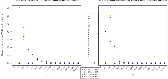
in 6, . . . , 20. The absolute variation of the VaR and the CVaR values with respect to 𝑁
is given in Figure 2. We conclude that the VaR𝑎p𝐻q is stable from 𝑁 “16 384 and that
CVaR𝑎p𝐻q is stable from 𝑁 “8 192. The CVaR converges faster because it is a minimum,
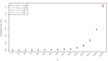
while the VaR is an argmin. The CPU computing time of the method is illustrated in
0 5 10 15 20 25 30 35
VaR convergence in Black and Scholes model
N Absolute variation of V aRa (( ST − K )+ ) 64 128 256 512 1024 2048 4096 8192 16384 32768 65536 131072 262144 5242881048576 T = 0.5, a = 0.99 T = 0.5, a = 0.95 T = 1, a = 0.99 T = 1, a = 0.95 0 1 2 3 4 5
CVaR convergence in Black and Scholes model
N Absolute variation of CV aR a (( ST − K )+ ) 64 128 256 512 1024 2048 4096 8192 16384 32768 65536 131072 262144 5242881048576
Figure 2: The absolute variation ofVaR𝑎pp𝑆𝑇´𝐾q`q andCVaR𝑎pp𝑆𝑇´𝐾q`q with respect
to 𝑁 under Black and Scholes model.
0.0 0.2 0.4 0.6 0.8 1.0 1.2
Computing time of VaR/CVaR in Black and Scholes model
N Compting time (sec) 64 128 256 512 1024 2048 4096 8192 16384 32768 65536 131072 262144 524288 1048576 T = 0.5, a = 0.99 T = 0.5, a = 0.95 T = 1, a = 0.99 T = 1, a = 0.95
7.2 Merton model
This model is proposed by [34]. The price is described by an exponential Lévy process (1) where 𝑋𝑡“ 𝛾𝑡 ` 𝜎𝐵𝑡` 𝑁𝑡 ÿ 𝑖“1 𝑌𝑖,
with 𝛾 P R, p𝐵𝑡q𝑡Pr0,𝑇 s is a standard Brownian motion, p𝑁𝑡q𝑡Pr0,𝑇 s is a Poisson process with
intensity 𝜆 and p𝑌𝑖q𝑖ě1 are i.i.d. Gaussian random variables with parameters 𝑚 and 𝛿2.
For each 0 ď 𝑡 ď 𝑇 , the characteristic function of 𝑋 is given by
Φ𝑡p𝑢q “ Er𝑒𝑖𝑢𝑋𝑡s “ 𝑒𝑡Ψp𝑢q, and Ψp𝑢q “ 𝑖𝛾𝑢 ´ 𝜎 2 2 𝑢 2 ` 𝜆 ˆ exp ˆ 𝑖𝑚𝑢 ´𝛿 2 2𝑢 2 ˙ ´1 ˙ . Define 𝜈p𝑥q “ 𝜆 ˆ ?1 2𝜋𝛿exp ˆ ´p𝑥 ´ 𝑚q 2 2𝛿2 ˙ , 𝑥 P R and 𝑏 “ 𝛾 ` ż |𝑥|ď1 𝑥 𝜈pd𝑥q.
Then, Ψ can be written on the form
Ψp𝑢q “ 𝑖𝛾𝑢 ´𝜎 2 2 𝑢 2 ` ż R `𝑒𝑖𝑢𝑥 ´1˘ 𝜈pd𝑥q “ 𝑖𝑏𝑢 ´𝜎 2 2 𝑢 2 ` ż R `𝑒𝑖𝑢𝑥 ´1 ´ 𝑖𝑢𝑥1|𝑥|ď1˘ 𝜈pd𝑥q.
We conclude that, under P, p𝑋𝑡q𝑡Pr0,𝑇 s is a Lévy process with triplet p𝑏, 𝜎2, 𝜈q. With
this model, the market is incomplete. The compound Poisson process makes the risk uncontrolled and there exists an infinity of equivalent martingale measures. Estimation of different parameters from financial data is detailed in [46].
Esscher martingale measure. The exponential moment Er𝑒𝜃𝑋1s is finite for all 𝜃 P R.
To prove the existence of the Esscher martingale measure P˚, we look for a real 𝜃 P R
solution to 𝛾 ` 𝜎2𝜃 ` 𝜎2 2 ` ż R 𝑒𝜃𝑥 p𝑒𝑥´1q 𝜈pd𝑥q “ 𝑟, or farther 𝛾 ` 𝜎2𝜃 ` 𝜎 2 2 ` 𝜆 ´ 𝑒𝑚p𝜃`1q`𝛿22p𝜃`1q2 ´ 𝑒𝑚𝜃`𝛿22𝜃2 ¯ “ 𝑟.
For numerical application with the parameters given in Table 1, we obtain 𝜃 « ´0.352.
The characteristic function of p𝑋𝑡q𝑡Pr0,𝑇 s under P˚ is given by
Φ˚ 𝑡p𝑢q “ 𝑒 𝑡Ψ˚p𝑢q , where Ψ˚ p𝑢q “ 𝑖p𝛾 ` 𝜎2𝜃q𝑢 ´ 𝜎 2 2 𝑢 2 ` 𝜆 ´ 𝑒𝑚p𝜃`𝑖𝑢q`𝛿22p𝜃`𝑖𝑢q2 ´ 𝑒𝑚𝜃`𝛿22𝜃2 ¯ .
We conclude that, with the Esscher martingale measure, we are able to provide analytic expression of the characteristic function under an equivalent martingale measure. This analytic form will be numerically inverted later with the fast Fourier transform to provide the option price.
Using Proposition 2.1, the process p𝑋𝑡q𝑡Pr0,𝑇 s is a Lévy process under P˚ with triplet
p𝑏˚, 𝜎2, 𝜈˚q defined by 𝑏˚ “ 𝛾 ` 𝜎2𝜃 ` ż |𝑥|ď1 𝑥𝜈˚ pd𝑥q and 𝜈˚ p𝑥q “ 𝑒𝜃𝑥𝜈p𝑥q “ 𝜆˚ˆ?1 2𝜋𝛿exp p𝑥 ´ p𝑚 ` 𝛿 2𝜃qq2{p2𝛿2 q, where 𝜆˚
“ 𝜆expp𝑚𝜃 ` 𝛿22𝜃2q. Hence, the Esscher martingale model p𝑋𝑡q𝑡Pr0,𝑇 s is once
again a jump diffusion with compound Poisson jumps:
𝑋𝑡“ p𝛾 ` 𝜎2𝜃q𝑡 ` 𝜎𝐵˚𝑡 ` 𝑁˚ 𝑡 ÿ 𝑖“1 𝑌˚ 𝑖 , where p𝐵˚
𝑡q𝑡Pr0,𝑇 s is a P˚-standard Brownian motion, p𝑁𝑡˚q𝑡Pr0,𝑇 s is a P˚-Poisson process
with intensity𝜆˚and p𝑌˚
𝑖 q𝑖ě1are i.i.d. Gaussian random variables with parameters𝑚`𝛿2𝜃
and 𝛿2.
Minimal entropy martingale measure. The existence of the minimal entropy
mar-tingale measure P: is equivalent to the existence of a real 𝛽 solution to
𝛾 ` 𝜎2𝛽 `𝜎2 2 ` ż R ` p𝑒𝑥´1q𝑒𝛽p𝑒𝑥´1q˘ 𝜈pd𝑥q “ 𝑟,
in the Merton model framework. With the same parameters of Table 1, we get numerically 𝛽 « ´0.365.
Using Theorem 3.2, p𝑋𝑡q𝑡Pr0,𝑇 sis a Lévy process under P:with triplet p𝑏:, 𝜎2, 𝜈:q defined
by 𝑏: “ 𝛾 ` 𝜎2𝛽 ` ż |𝑥|ď1 𝑥𝜈:pd𝑥q and 𝜈: p𝑥q “ 𝑒𝛽p𝑒𝑥´1q𝜈p𝑥q “ 𝜆:𝜌:p𝑥q where 𝜆:
“ş 𝜈:pd𝑥q and 𝜌:p𝑥q “ ş 𝜈𝜈::p𝑥qpd𝑥q. Hence, the minimal entropy martingale model
p𝑋𝑡q𝑡Pr0,𝑇 s is once again a jump diffusion with compound Poisson jumps:
𝑋𝑡 “ p𝛾 ` 𝜎2𝛽q𝑡 ` 𝜎𝐵𝑡:` 𝑁𝑡: ÿ 𝑖“1 𝑌: 𝑖 ,
where p𝐵𝑡:q𝑡Pr0,𝑇 sis a P:-standard Brownian motion, p𝑁𝑡:q𝑡Pr0,𝑇 sis a P:-Poisson process with
intensity 𝜆: and p𝑌:
𝑖 q𝑖ě1are i.i.d. random variables with probability density function 𝜌:.
The role of the damping factor 𝑒𝜃𝑥 in the case of the Esscher martingale measure P˚
and the dumping factor𝑒𝛽p𝑒𝑥
´1q in the case of the minimal entropy martingale measure P:
is to mitigate the general trend of the log price. In the Merton model, the general trend is
parameters 𝜃 and 𝛽 which permit to give more weight to negative jumps and less weight
to positive jumps in the Lévy densities 𝜈˚ and𝜈:. This rebalances the market in the
risk-neutral world and gives the martingale property. Conversely, if the log price expectation is negative, the dumping factors will strongly reduce the left tail of the risk-neutral Lévy densities.
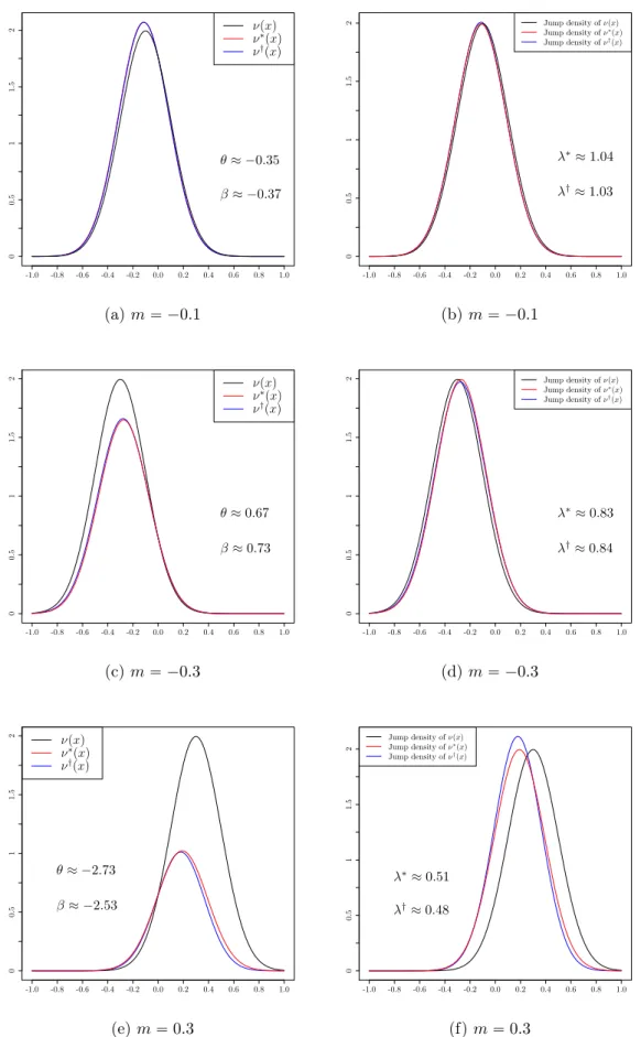
The initial Lévy density𝜈 and the two risk-neutral Lévy densities 𝜈˚(under the Esscher
martingale measure P˚) and 𝜈: (under the minimal entropy martingale measure P:), as
well as the corresponding jump densities, are depicted in Figure 4 for different values of the
log price expectation. We vary the jump size expectation 𝑚 “ t´0.1, ´0.3, 0.3u to have
different signs of Er𝑋𝑡s and therefore different signs of 𝜃 and 𝛽. The remaining parameters
of the model are the ones given in Table 1. Depending on the Esscher parameter sign, we have a dumping of the right tail or the left tail of the risk-neutral Lévy density. Despite this dumping effect in the Lévy densities, we observe in the right hand figures that the jump size densities are not affected by this change of measures and the main effect is then
an increase or decrease in the jump intensities 𝜆˚ and 𝜆:.
On the other hand, when we compare𝜈˚ to𝜈:, we find that both functions are almost
equal with variations that do not exceed 1.6 ˆ 10´2. We can explain this by the fact
that 𝑋 and ˆ𝑋 represent respectively the compound and the simple returns of the stock
price. So, we consider models with small jump𝑥 for which 𝑒𝑥
´1 « 𝑥. Thus, the Esscher
martingale measure and the minimal entropy martingale measure are almost the same.
While we have the triplet of p𝑋𝑡q𝑡Pr0,𝑇 s under the minimal entropy martingale
mea-sure, we still do not have an analytic expression of the characteristic function under this measure. For that, using the FFT to compute option prices under the minimal entropy martingale measure will be not possible.
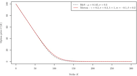
Pricing with FFT under the Esscher martingale measure. In Figure 5, we
com-pare the option price under a Black and Scholes model and a Merton model having the
same expectation of p𝑋𝑡q𝑡Pr0,𝑇 s. We choose models parameters such that𝜇 ´𝜎
2
2 “ 𝛾 ` 𝜆𝑚.
The numerical computation of the call price with respect to the strike 𝐾, is presented in
Figure 5. As the Merton model allows bigger negative jumps, the probability to finish in-the-money is smaller. Otherwise, the option price can always be written
𝐶p𝐾q “ 𝑆0Π1´ 𝐾𝑒´𝑟𝑇Pp𝑆𝑇 ą 𝐾q,
where Π1 is the delta of the option. The call price is thus greater around the money in
the Merton model.
Option price sensitivity to jumps. To discuss the effects of jumps on the option
price, we compare the results of the Merton model with respect to the jump intensity. Recall that the Black and Scholes model and the Merton model are exponential Lévy
models with triplets p𝜇 ´ 𝜎22, 𝜎2, 0q and p𝛾 `ş
|𝑥|ď1𝑥𝜈pd𝑥q, 𝜎 2, 𝜈q respectively, where 𝜈p𝑥q “ 𝜆 ˆ?1 2𝜋𝛿 exp ` p𝑥 ´ 𝑚q2{p2𝛿2q˘ .
Then, a Black and Scholes model is a Merton model with particular parameters 𝛾 “
𝜇 ´ 𝜎2
2 and 𝜆 “ 0. This model does not contain jumps as the jump intensity 𝜆 “ 0. To
see the effect of jumps on the option prices, we fix parameters such that 𝛾 “ 𝜇 ´ 𝜎2
2 and
compare the Black and Scholes model to Merton models with different jump intensities.
We take the parameters of Table 1 except for 𝜆 that varies in t2, 4, 6u. Note that this
choice of parameters respects the condition 𝛾 “ 𝜇 ´ 𝜎2
ν(x) ν∗(x) ν†(x) θ≈ −0.35 β≈ −0.37 -1.0 -0.8 -0.6 -0.4 -0.2 0.0 0.2 0.4 0.6 0.8 1.0 0 0.5 1 1.5 2 (a) 𝑚 “ ´0.1 Jump density of ν(x) Jump density of ν∗(x) Jump density of ν†(x) λ∗≈ 1.04 λ†≈ 1.03 -1.0 -0.8 -0.6 -0.4 -0.2 0.0 0.2 0.4 0.6 0.8 1.0 0 0.5 1 1.5 2 (b) 𝑚 “ ´0.1 ν(x) ν∗(x) ν†(x) θ≈ 0.67 β≈ 0.73 -1.0 -0.8 -0.6 -0.4 -0.2 0.0 0.2 0.4 0.6 0.8 1.0 0 0.5 1 1.5 2 (c) 𝑚 “ ´0.3 Jump density of ν(x) Jump density of ν∗(x) Jump density of ν†(x) λ∗≈ 0.83 λ†≈ 0.84 -1.0 -0.8 -0.6 -0.4 -0.2 0.0 0.2 0.4 0.6 0.8 1.0 0 0.5 1 1.5 2 (d) 𝑚 “ ´0.3 ν(x) ν∗(x) ν†(x) θ≈ −2.73 β≈ −2.53 -1.0 -0.8 -0.6 -0.4 -0.2 0.0 0.2 0.4 0.6 0.8 1.0 0 0.5 1 1.5 2 (e) 𝑚 “ 0.3 Jump density of ν(x) Jump density of ν∗(x) Jump density of ν†(x) λ∗≈ 0.51 λ†≈ 0.48 -1.0 -0.8 -0.6 -0.4 -0.2 0.0 0.2 0.4 0.6 0.8 1.0 0 0.5 1 1.5 2 (f) 𝑚 “ 0.3
Figure 4: Lévy densities and jump size densities under the historical measure, the Esscher martingale measure and the minimal entropy martingale measure in the Merton model.
0 50 100 150 200 250 300 0 20 40 60 80 100 Strike K Option price C (K ) B&S : µ = 0.145, σ = 0.3 Merton : γ = 0.2, σ = 0.3, λ = 1, m = −0.1, δ = 0.2
Figure 5: Option price with respect to the strike 𝐾. A comparison between a Black and
Scholes model and a Merton model with the same expectation 𝜇 ´ 𝜎2{2 “ 𝛾 ` 𝜆𝑚.
presented in Figure 6a. For all models, the option price approaches 𝑆0 as 𝐾 Ñ 0 and
goes to 0 as 𝐾 Ñ `8. The jump intensity modifies the option price only for strikes
around at-the-money. Otherwise, as the intensity increases, we have more jumps in the
period r0, 𝑇 s and the variance Varp𝑋𝑡q “ p𝜎2` 𝜆p𝑚2` 𝛿2qq 𝑡 increases. Consequently, the
option price increases due to the greater risk that jumps bring to the seller. The same observation is found when the jump size volatility increases. We present it in Figure 6b. The price with respect to the jump size mean is given by Figure 6c. With a negative average of jumps size in the asset price, we have interesting out-the-money options, while in-the-money options are less interesting. A positive average of jumps size leads to reverse statement.
Risk measurement. We compute the VaR and the CVaR of the payoff in the Merton
model framework. With the parameters of Table 1 and a strike 𝐾 “ 110, we illustrate
the sensitivity of VaR and CVaR computing with respect to the size of discretization grid
in Figures 7 and 8. In Figure 7, we give VaR𝑎p𝐻q and CVaR𝑎p𝐻q for different values of
𝑁 , while in Figure 8, we show the absolute variation of the VaR and the CVaR values
with respect to 𝑁 . For the different chosen values of 𝑇 and 𝑎, VaR𝑎p𝐻q is stable from
𝑁 “ 16 384 and the CVaR𝑎p𝐻q converges from 𝑁 “ 2 048. The CPU computing time
of the method is given in Figure 9. Up to 𝑁 “ 16 384, the algorithm is considered as
instantaneous.
7.3 Variance gamma model
The variance gamma process is proposed by [33] to describe stock price dynamics istead of the Brownian motion in the original Black and Scholes model. Two new parameters: 𝑚 skewness and 𝜅 kurtosis are introduced in order to describe asymmetry and fat tails of real life distributions. A variance gamma process is obtained by evaluating a Brownian motion with a drift at a random time given by a gamma process.
Definition 7.1. The variance gamma (VG) process p𝑌𝑡q𝑡Pr0,𝑇 s with parameters p𝑚, 𝛿, 𝜅q
is defined as
0 50 100 150 200 250 300 0 20 40 60 80 100 Strike K Option price C (K ) λ = 0 λ = 2 λ = 4 λ = 6
(a) Sensitivity to the jump intensity
80 100 120 140 160 0 5 10 15 20 25 Strike K Option price C (K ) δ = 0.1 δ = 0.2 δ = 0.4
(b) Sensitivity to the jump size variance
80 100 120 140 160 0 5 10 15 20 25 Strike K Option price C (K ) m =−0.1 m =−0.3 m = 0.3
(c) Sensitivity to the jump size mean
Figure 6: Call price sensitivity to the parameters of Merton model.
where p𝐵𝑡q𝑡Pr0,𝑇 s is a standard Brownian motion and p𝛾𝑡q𝑡Pr0,𝑇 s is a gamma process with
unit mean rate and variance rate 𝜅.
Proposition 7.1. The VG process p𝑌𝑡q𝑡Pr0,𝑇 s is a Lévy process with characteristic
func-tion Φ𝑡 and characteristic triplet p
ş |𝑥|ď1𝑥𝜈pd𝑥q, 0, 𝜈q where Er𝑒𝑖𝑢𝑌𝑡s “ ˆ 1 1 ´ 𝑖𝑚𝜅𝑢 ` p𝛿2𝜅{2q𝑢2 ˙𝑡{𝜅 and 𝜈p𝑥q “ 1 𝜅|𝑥|exp ¨ ˝ 𝑚 𝛿2𝑥 ´ b 𝑚2 𝛿2 ` 2 𝜅 𝛿 |𝑥| ˛ ‚.
From the expression of 𝜈, there exists infinitely small jumps. Such a process is called
an infinite activity process. It does not admit a distribution of jump size since jumps happen infinitely.
To describe the stock price, we just add a drift component to the VG process. A Brownian component is not necessary and the process moves essentially by jumps. The price process is defined by an exponential Lévy model (1) where
𝑋𝑡“ 𝛾𝑡 ` 𝑌𝑡.
The process p𝑋𝑡q𝑡Pr0,𝑇 sis a Lévy process with characteristic triplet
´
40 60 80 100 120 140
VaR of payoff in Merton model
N V aR a (( ST − K )+ ) 64 128 256 512 1024 2048 4096 8192 16384 32768 65536131072 262144 5242881048576 T = 0.5, a = 0.99 T = 0.5, a = 0.95 T = 1, a = 0.99 T = 1, a = 0.95 40 60 80 100 120 140
CVaR of payoff in Merton model
N CV aR a (( ST − K )+ ) 64 128 256 512 1024 2048 4096 8192 16384 32768 65536131072 262144 5242881048576
Figure 7: VaR𝑎pp𝑆𝑇 ´ 𝐾q`q and CVaR𝑎pp𝑆𝑇 ´ 𝐾q`q with respect to 𝑁 under a Merton
model. 0 5 10 15 20 25 30 35
VaR convergence in Merton model
N Absolute variation of V aRa (( ST − K )+ ) 64 128 256 512 1024 2048 4096 8192 16384 32768 65536131072 262144 5242881048576 T = 0.5, a = 0.99 T = 0.5, a = 0.95 T = 1, a = 0.99 T = 1, a = 0.95 0 2 4 6
CVaR convergence in Merton model
N Absolute variation of CV aR a (( ST − K )+ ) 64 128 256 512 1024 2048 4096 8192 16384 32768 65536131072 262144 5242881048576
Figure 8: The absolute variation ofVaR𝑎pp𝑆𝑇´𝐾q`q andCVaR𝑎pp𝑆𝑇´𝐾q`q with respect
0.0 0.2 0.4 0.6 0.8 1.0 1.2
Computing time of VaR/CVaR in Merton model
N Compting time (sec) 64 128 256 512 1024 2048 4096 8192 16384 32768 65536 131072 262144 524288 1048576 T = 0.5, a = 0.99 T = 0.5, a = 0.95 T = 1, a = 0.99 T = 1, a = 0.95
Figure 9: CPU time of the VaR/CVaR computing method under a Merton model. and characteristic function given by
Φ𝑡p𝑢q “ Er𝑒𝑖𝑢𝑋𝑡s “
𝑒𝑖𝛾𝑢𝑡
p1 ´ 𝑖𝑚𝜅𝑢 ` p𝛿2𝜅{2q𝑢2q𝑡{𝜅.
The procedure to fit the variance gamma model to financial data is explained in [45].
Esscher martingale measure. By solving the inequality 1 ´ 𝑖𝑚𝜅𝑢 ` p𝛿2𝜅{2q𝑢2 ą 0
with respect to𝑢, we show that 𝑋𝑡for some𝑡 or, equivalently, for all 𝑡, possesses a moment
generating function 𝑢 ÞÑ Erexpp𝑢𝑋𝑡qs on
´
´𝑚{𝛿2´a𝑚2{𝛿2`2{𝜅 𝛿, ´𝑚{𝛿2`a𝑚2{𝛿2`2{𝜅 𝛿
¯ .
To apply Theorem 3.1, we assume that 2a𝑚2{𝛿2`2{𝜅 𝛿 ą 1. Under this assumption,
we look for 𝜃 P ´ ´𝑚{𝛿2´a𝑚2{𝛿2`2{𝜅 𝛿, ´𝑚{𝛿2`a𝑚2{𝛿2`2{𝜅 𝛿 ´ 1 ¯ solution to E“𝑒p𝜃`1q𝑋𝑡‰“ 𝑒𝑟𝑡E“𝑒𝜃𝑋𝑡‰ .
For the parameters given in Table 1, the moment generating function of 𝑋𝑡 is well
defined on p´3.15, 3.17q. Numerically, we obtain 𝜃 “ ´0.57.
The characteristic function of p𝑋𝑡q𝑡Pr0,𝑇 s under P˚ is given by
Φ˚ 𝑡p𝑢q “ Er𝑒p𝜃`𝑖𝑢q𝑋𝑡s Er𝑒𝜃𝑋𝑡s “ 𝑒𝑖𝛾𝑢𝑡 `1 ´ 𝑖𝑚˚𝜅𝑢 ` p𝛿˚2𝜅{2q𝑢2˘𝑡{𝜅, where𝑚˚ “ p𝑚 ` 𝛿2𝜃q{𝐴, 𝛿˚ “ 𝛿{ ? 𝐴 and 𝐴 “ 1 ´ 𝑚𝜅𝜃 ´𝛿2𝜅 2 𝜃 2. Hence, p𝑋 𝑡q𝑡Pr0,𝑇 s is once
again a variance gamma process under P˚ with characteristic triplet p𝛾`ş
|𝑥|ď1𝑥𝜈˚pd𝑥q,0,𝜈˚q where 𝜈˚ p𝑥q “ 𝑒𝜃𝑥𝜈p𝑥q “ 1 𝜅|𝑥|exp ¨ ˝ 𝑚˚ 𝛿˚2𝑥 ´ b 𝑚˚2 𝛿˚2 ` 2 𝜅 𝛿˚ |𝑥| ˛ ‚.
The initial Lévy density and the risk-neutral Lévy density are given in Figure 10. With
our choice of parameters, the general trend Er𝑋𝑡s “ p𝛾 ` 𝑚q𝑡 is positive, which leads to
a negative 𝜃. The large positive jumps will be nearly irrelevant for pricing options, while
0 20 40 60 80 ν∗(x) ν(x) -0.8 -0.6 -0.4 -0.2 0.0 0.2 0.4 0.6 0.8
Figure 10: The risk neutral Lévy density 𝜈˚p𝑥q of the Esscher martingale measure in the
variance gamma model, compared to the initial Lévy density 𝜈p𝑥q.
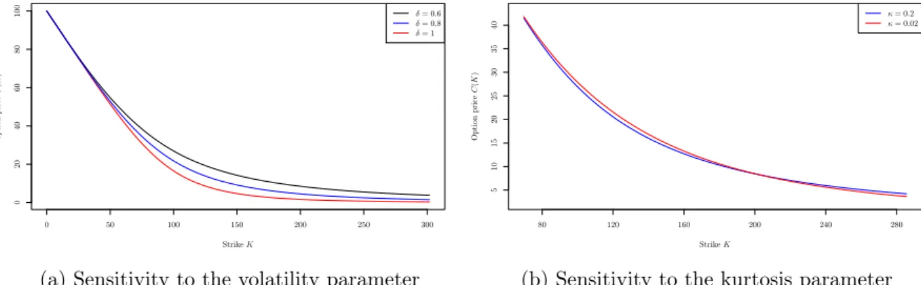
Pricing with FFT under the Esscher martingale measure. The explicit form of
the characteristic function under the Esscher martingale measure P˚ is applied to price
call options. Figures 11a and 11b represent the sensitivity of the call price to a variation
of the parameters 𝛿 and 𝜅 respectively. We take the parameters of Table 1 except for 𝛿
that varies in t0.6, 0.8, 1u in Figure 11a and 𝜅 that varies in t0.02, 0.2u in Figure 11b. The
parameters 𝛿 and 𝜅 provide control over volatility and kurtosis respectively. Increasing 𝛿
leads to greater volatility which in turn increases the option price. On the other hand,
when 𝜅 inscreases, the distribution tails of the asset price become fatter and the price of
the out-the-money call increases, while the price of the at-the-money option decreases.
0 50 100 150 200 250 300 0 20 40 60 80 100 Strike K option price C (K ) δ = 0.6 δ = 0.8 δ = 1
(a) Sensitivity to the volatility parameter
Strike K Option price C (K ) 80 120 160 200 240 280 5 10 15 20 25 30 35 40 κ = 0.2 κ = 0.02
(b) Sensitivity to the kurtosis parameter
Figure 11: Call price sensitivity to the parameters of the variance gamma model.
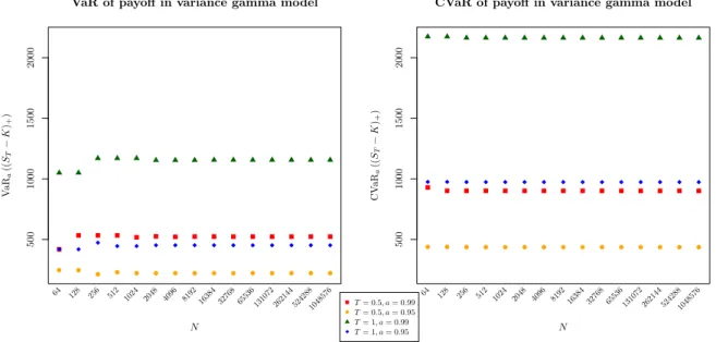
Risk measurement. We compute the VaR and the CVaR of the payoff under a variance
gamma model. With the parameters of Table 1 and a strike 𝐾 “ 110, we illustrate the
sensitivity of VaR and CVaR computing with respect to the size of discretization grid in
Figures 12 and 13. In Figure 12, we give VaR𝑎p𝐻q and CVaR𝑎p𝐻q for different values of
𝑁 , while in Figure 13, we show the absolute variation of the VaR and the CVaR values
with respect to 𝑁 . For different values of 𝑇 and 𝑎, VaR𝑎p𝐻q is stable from 𝑁 “ 16 384
500
1000
1500
2000
VaR of payoff in variance gamma model
N V aR a (( ST − K )+ ) 64 128 256 512 1024 2048 4096 8192 16384 32768 65536131072 262144 5242881048576 T = 0.5, a = 0.99 T = 0.5, a = 0.95 T = 1, a = 0.99 T = 1, a = 0.95 500 1000 1500 2000
CVaR of payoff in variance gamma model
N CV aR a (( ST − K )+ ) 64 128 256 512 1024 2048 4096 8192 16384 32768 65536131072 262144 5242881048576
Figure 12: VaR𝑎pp𝑆𝑇 ´ 𝐾q`q and CVaR𝑎pp𝑆𝑇´ 𝐾q`q with respect to 𝑁 under a variance
gamma model.
is given in Figure 14. Up to 𝑁 “ 16 384, the algorithm is considered as instantaneous.
We conclude that for the three models, the value𝑁 “ 16384 permits to give a stable
value of both VaR𝑎p𝐻q and CVaR𝑎p𝐻q, with a negligible computing time.
8
Conclusion
In this survey, we studied step by step how to price European option under an Exponen-tial Lévy model. We used the Esscher transform technique to construct two equivalent martingale measures: the Esscher martingale measure and the minimal entropy martin-gale measure. From the observation that the compound return and the simple return of a stock price process are very close, we showed that these two measures are almost similar. However, the minimal entropy martingale measure is not adequate to the Carr-Madan pricing method as the characteristic function under this latter does not have an analytic expression, even in simple models. Under the Esscher martingale measure, we numerically computed the price of European option using the Carr-Madan method based on the fast Fourier transform. Numerical error of the Carr-Madan method is shown with comparison to the closed-form formula in the Black and Scholes context. Moreover, the sensitivity of option price to jumps is presented in the Merton model and the variance gamma model with respect to jump parameters. Finally, applications of Fourier inversion technique in Risk measurement are proposed to compute the VaR and the CVaR of derivatives, as well as the VaR and the CVaR of monetary loss and loss in terms of returns.
References
[1] C. Acerbi and D. Tasche. On the coherence of expected shortfall. Journal of Banking & Finance, 26(7):1487–1503, 2002.
[2] D. Applebaum. Lévy processes and stochastic calculus. Cambridge University Press, 2009.
0 20 40 60 80 100 120
VaR convergence in variance gamma model
N Absolute variation of V aR a (( ST − K )+ ) 64 128 256 512 1024 2048 4096 8192 16384 32768 65536131072 262144 5242881048576 T = 0.5, a = 0.99 T = 0.5, a = 0.95 T = 1, a = 0.99 T = 1, a = 0.95 0 5 10 15 20 25
CVaR convergence in variance gamma model
N Absolute variation of CV aRa (( ST − K )+ ) 64 128 256 512 1024 2048 4096 8192 16384 32768 65536131072 262144 5242881048576
Figure 13: The absolute variation of VaR𝑎pp𝑆𝑇 ´ 𝐾q`q and CVaR𝑎pp𝑆𝑇 ´ 𝐾q`q with
respect to 𝑁 under a variance gamma model.
0.0
0.5
1.0
1.5
Computing time of VaR/CVaR in variance gamma model
N Compting time (sec) 64 128 256 512 1024 2048 4096 8192 16384 32768 65536 131072 262144 524288 1048576 T = 0.5, a = 0.99 T = 0.5, a = 0.95 T = 1, a = 0.99 T = 1, a = 0.95
Figure 14: CPU time of the VaR/CVaR computing method under a variance gamma model.