LETTER • OPEN ACCESS
Evaluating changes of biomass in global
vegetation models: the role of turnover fluctuations
and ENSO events
To cite this article: Anselmo García Cantú et al 2018 Environ. Res. Lett. 13 075002
View the article online for updates and enhancements.
Related content
Benchmarking carbon fluxes of the ISIMIP2a biome models
-Photosynthetic productivity and its efficiencies in ISIMIP2a biome models: benchmarking for impact assessment studies
-Regional contribution to variability and trends of global gross primary productivity
-Recent citations
Pronounced and unavoidable impacts of low-end global warming on northern high-latitude land ecosystems
Akihiko Ito et al
LETTER
Evaluating changes of biomass in global vegetation
models: the role of turnover fluctuations and ENSO events
Anselmo Garc´ıa Cant́u1,11 , Katja Frieler1, Christopher P O Reyer1, Philippe Ciais2, Jinfeng Chang2,Akihiko Ito3, Kazuya Nishina3, Louis Franc¸ois4, Alexandra-Jane Henrot4, Thomas Hickler5, J¨org
Steinkamp5,10, Rashid Rafique6, Fang Zhao1 , Sebastian Ostberg1 , Sibyll Schaphoff1, Hanqin Tian7,
Shufen Pan7, Jia Yang7, Catherine Morfopoulos8and Richard Betts8,9 1 Potsdam Institute for Climate Impact Research, D-14412 Potsdam, Germany
2 Laboratoire des Sciences du Climat et de l’Environnement, UMR8212, CEA-CNRSUVSQ, 91191 Gif-sur-Yvette, France 3 National Institute for Environmental Studies, Tsukuba, Ibaraki 305–8506, Japan
4 Unit´e de Mod´elisation du climat et des Cycles Biog´eochimiques, UR SPHERES, Universit´e de Li`ege, Quartier Agora, All´ee du Six Aôut
19 C, B-4000 Li`ege, Belgium
5 Senckenberg Biodiversity and Climate Research Centre (BiK-F), Frankfurt am Main, Germany
6 Joint Global Change Research Institute, Pacific Northwest National Lab, College Park, MD, United States of America
7 International Center for Climate and Global Change Research, School of Forestry and Wildlife Sciences, Auburn University, Auburn,
AL, United States of America
8 College of Life and Environmental Sciences, University of Exeter, Exeter EX4 4QE, United Kingdom 9 Met Office, Exeter, Devon EX1 3PB, United Kingdom
10 Zentrum f¨ur Datenverarbeitung, Johannes Gutenberg-Universit¨at Mainz, Germany 11 Author to whom any correspondence should be addressed.
OPEN ACCESS
RECEIVED 3 March 2018 ACCEPTED FOR PUBLICATION 18 May 2018 PUBLISHED 26 June 2018
Original content from this work may be used under the terms of the Creative Commons Attribution 3.0 licence. Any further distribution of this work must maintain attribution to the author(s) and the title of the work, journal citation and DOI.
E-mail:anselmogarciacantu@gmail.com
Keywords: terrestrial ecosystems, ENSO, interannual variability, vegetation optical depth, biomass, ISIMIP2a, global vegetation models Supplementary material for this article is availableonline
Abstract
This paper evaluates the ability of eight global vegetation models to reproduce recent trends and
inter-annual variability of biomass in natural terrestrial ecosystems. For the purpose of this
evaluation, the simulated trajectories of biomass are expressed in terms of the relative rate of change in
biomass (RRB), defined as the deviation of the actual rate of biomass turnover from its equilibrium
counterpart. Cumulative changes in RRB explain long-term changes in biomass pools. RRB
simulated by the global vegetation models is compared with its observational equivalent, derived from
vegetation optical depth reconstructions of above-ground biomass (AGB) over the period 1993–2010.
According to the RRB analysis, the rate of global biomass growth described by the ensemble of
simulations substantially exceeds the observation. The observed fluctuations of global RRB are
significantly correlated with El Ni
̃no Southern Oscillation events (ENSO), but only some of the
simulations reproduce this correlation. However, the ENSO sensitivity of RRB in the tropics is not
significant in the observation, while it is in some of the simulations. This mismatch points to an
important limitation of the observed AGB reconstruction to capture biomass variations in tropical
forests. Important discrepancies in RRB were also identified at the regional scale, in the tropical
forests of Amazonia and Central Africa, as well as in the boreal forests of north-western America,
western and central Siberia. In each of these regions, the RRBs derived from the simulations were
analyzed in connection with underlying differences in net primary productivity and biomass turnover
rate —as a basis for exploring in how far differences in simulated changes in biomass are attributed to
the response of the carbon uptake to CO
2increments, as well as to the model representation of factors
affecting the rates of mortality and turnover of foliage and roots. Overall, our findings stress the
usefulness of using RRB to evaluate complex vegetation models and highlight the importance of
conducting further evaluations of both the actual rate of biomass turnover and its equilibrium
counterpart, with special focus on their background values and sources of variation. In turn, this task
would require the availability of more accurate multi-year observational data of biomass and net
primary productivity for natural ecosystems, as well as detailed and updated information on
land-cover classification.
1. Introduction
Large uncertainties of the global carbon budget (Le Qu´er´e et al 2015) are associated with the terrestrial carbon cycle (Bloom et al 2016). Reducing those uncertainties requires an improved capacity to esti-mate the fluxes of carbon between the atmosphere and terrestrial ecosystems, along with gaining better understanding of the dynamics of the correspond-ing carbon pools and their sensitivity to climate. For this purpose, global vegetation models (GVMs) have been developed to describe the effects of climate, atmospheric CO2and other drivers on a large num-ber of ecological processes, including photosynthesis, respiration, carbon allocation, phenology, and plant mortality which altogether control the dynamics of carbon pools. The possibility to evaluate the perfor-mance of such complex vegetation models is currently improving thanks to novel satellite-based observation methods.
Recently, the ensemble of GVMs available through the Inter-Sectoral Model Intercomparison Project Phase 2a (ISIMIP2a) has been evaluated with regards to the models’ ability to reproduce the historical trends and variability of the gross primary production and net biome productivity (Ito et al 2017, Chang et al 2017, Chen et al2017). Using the same ensemble of GVMs, this paper aims at corroborating recent trends and interannual variations of biomass stocks. Beyond comparing changes in biomass, derived from GVMs and observations, we propose to address the processes explaining these changes. As recently shown, the equi-librium turnover rate of biomass (TRB) Thurner et al (2017) and the rate of loss of biomass (RLB) (Friend
et al 2014, Bloom et al 2016) are major sources of uncertainty in model representations of biomass dynamics. The RLB is the inverse of the residence time of carbon in vegetation, i.e. the time carbon remains in living biomass pools from fixation to removal. In natural ecosystems, biomass removal occurs through background mortality of stems, foliage and roots, and through losses from disturbances such as fire, storm or insect damage. The TRB is defined as the value of RLB when the biomass pool is in equilibrium, i.e. the inverse of the equilibrium residence time.
The objective of this paper is to analyze changes in biomass stocks from the view point of the deviations of the biomass loss flux, from the loss in the virtual equilibrium state, i.e. the difference between TRB and RLB. This difference, here referred as the relative rate of change in biomass (RRB), is relevant for model eval-uation since a positive/negative value in the temporal mean of RRB entails that the biomass system tends to move towards its equilibrium following an expo-nential increase/decrease in biomass. Observed RRB is diagnosed from annual maps of biomass retrieved from vegetation optical depth satellite observations (Liu
et al2015) during the period 1993–2010. We note that this product may be less accurate than other biomass
datasets, but it is the only temporally resolved one allowing for comparison with model outputs on annual time-scale.
We focus on the variations of processes control-ling biomass change in so called ‘natural’ terrestrial ecosystems, i.e. in ecosystems not being affected by land use change. For this purpose, areas covered with cropland and pastures were filtered out from the grid-ded data of the observation and GVM simulations, prior to the analysis of RRB. At the global scale, this work evaluates the performance of GVMs to repro-duce the observed temporal mean of RRB. In addition, global biomass variations are evaluated with focus on the relation between RRB fluctuations and the El Nĩno Southern Oscillations (ENSO) that occurred since 1993.
The behavior of RRB in the models is further ana-lyzed in specific regions representative of the main for-est biomes (table S1 in supplementary information (SI) available at stacks.iop.org/ERL/13/075002/mmedia). The underlying differences in RRB in the GVM simu-lations are investigated in relation with the trends and variations of the net primary productivity (NPP) and RLB. In addition, the spatial share of regional biomass trends in the simulations is evaluated in terms of the land cover fraction where the temporal mean of RRB exhibits negative values –i.e. areas where the observa-tion indicates loss of biomass.
2. Datasets and methods
2.1. Datasets
2.1.1. The global vegetation model simulations
The simulations were performed by eight GVMs, namely, CARAIB (Warnant et al1994, G´erard et al 1999, Dury et al 2011), DLEM (Tian et al 2015), JULES-UoE (Best et al2011, Clark et al2011, Harper
et al 2016), LPJ-GUESS (Smith et al 2014), LPJmL (Bondeau et al 2007), ORCHIDEE (Krinner et al 2005), VEGAS (Zeng et al 2005), and VISIT (Ito and Inatomi 2012). These models embody different degrees of detail in the representation of biomass dynamics reflecting, productivity, allocation, main-tenance respiration, vegetation dynamics and losses from mortality and disturbances (see tables1and2). Each simulation was forced by a time-series of global atmospheric CO2concentration (Keeling and Whorf 2005) and historical reconstructions of climate on a 0.5◦global grid in daily temporal resolution. In addi-tion, simulations of all models, except CARAIB, were constrained with historical use maps. The land-use dataset describes cropland and pasture areas for the year 2000 (Ramankutty et al2008). Changes in cropland and pasture covers were extrapolated into past and future using the trends reported in HYDE3 (Goldewijk et al2011). A further detailed classifica-tion of crops and irrigated land was achieved using the MIRCA2000 crop dataset (Portmann et al2010).
Table 1. Summary of key processes represented in the global vegetation models used in this study: dynamical vegetation (DYNV), nitrogen limitation (NITL); CO2fertilization effect (CO2E); light interception (LIGI); light use efficiency (LIGU); phenology (PHEN); number of plant functional types in natural vegetation (#PFTS); water stress on photosynthesis (WASP); heat stress on photosynthesis (HEAP); evapo-transpiration (EVAT); differences in root depth (DROD); root distribution over depth (RDOD); closed energy balance (CBAL); latent heat (LATH); sensible heat (SENH); information non-specified (N/S) (for further details see ISIMIP2a,
https://esg.pik-potsdam.de/projects/isimip2a/).
MODELS DYNV NITL CO2E LIGI LIGU PHEN #PFTS WASP HEAP EVAT DROD RDOD CBAL LATH SENH
CARAIB ∙ — ∙ ∙ ∙ ∙ 26 ∙ ∙ ∙ — — ∙ ∙ ∙ DLEM — ∙ ∙ ∙ ∙ ∙ 14 ∙ ∙ ∙ — — — ∙ — JULES ∙ — ∙ ∙ ∙ ∙ 9 ∙ ∙ ∙ ∙ ∙ ∙ ∙ ∙ LPJ-GUESS ∙ ∙ ∙ ∙ ∙ ∙ 11 ∙ — ∙ — ∙ — — — LPJmL ∙ — ∙ ∙ ∙ ∙ 9 ∙ ∙ ∙ — ∙ ∙ ∙ ∙ ORCHIDEE ∙ — ∙ ∙ ∙ ∙ 10 ∙ ∙ ∙ ∙ ∙ ∙ ∙ ∙ VEGAS ∙ ∙ ∙ ∙ ∙ ∙ 4 ∙ — ∙ ∙ N/S ∙ ∙ ∙ VISIT — — ∙ ∙ — ∙ 26 ∙ ∙ ∙ ∙ ∙ — ∙ —
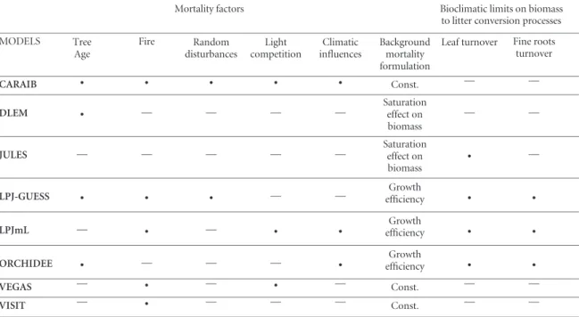
Table 2. Factors influencing the rate of biomass loss in the global vegetation models used in this study.
Mortality factors Bioclimatic limits on biomass to litter conversion processes MODELS Tree Age Fire Random disturbances Light competition Climatic influences Background mortality formulation
Leaf turnover Fine roots turnover
CARAIB ∙ ∙ ∙ ∙ ∙ Const. — —
DLEM ∙ — — — — Saturationeffect on
biomass
— —
JULES — — — — — Saturationeffect on
biomass
∙ —
LPJ-GUESS ∙ ∙ ∙ — — efficiencyGrowth ∙ ∙
LPJmL — ∙ — ∙ ∙ efficiencyGrowth ∙ ∙
ORCHIDEE ∙ — — — ∙ efficiencyGrowth ∙ ∙
VEGAS — ∙ — ∙ — Const. — —
VISIT — ∙ — — — Const. — —
All simulations were accomplished following a two-step process: (1) a ‘spin-up’ run in order to ensure that the carbon pools in the models reach an equilibrium, according to the climate, CO2 and land-use conditions at the beginning of the 20th century (1901–1930); (2) starting from year 1901, mod-els were forced away from equilibrium by historical climate, CO2 concentrations and land-use data, up to 2010 ( www.isimip.org/gettingstarted/#simulation-protocol). The model output used in this work covers the period 1971–2010.
One original feature of this study is the appli-cation of three different climate forcing datasets, instead of only one forcing usually used in other model inter-comparison projects (Sitch et al 2015, Huntzinger et al 2013). We consider the following climate forcing datasets: PGFv2 (http://hydrology. princeton.edu/data.pgf.php) (not available for VEGAS), GSWP3 (http://hydro.iis.u-tokyo.ac.jp/
GSWP3) and WFDEI (combined with WATCH)
(www.waterandclimatechange.eu/about/watch-forcin g-data-20th-century) (not available for JULES); The data pre-processing is described in section S1.1 in SI.
2.1.2. Gridded observation-based annual above-ground biomass dataset.
The above-ground biomass (AGB) inter-annual dataset used for model evaluation was produced by Liu et al (2015) by regressing satellite observations of vegeta-tion optical depth (VOD) with the map of tropical AGB from Saatchi et al (2011), VOD is an indicator of the water content of woody and leaf vegetation tis-sues, related to biomass. The VOD-AGB regression coefficients were used to extrapolate AGB on a grid of 0.25◦for each year during the period 1993–2012, based on annual maps of VOD. We re-gridded the Liu et al (2015) biomass dataset to the 0.5◦ resolution of the GVMs, using a conservative remapping algorithm (see details in S1.2 in SI).
2.1.3. Masking areas where biomass is affected by land use change
Since changes in land-use and land-cover drastically affect the turnover rate of carbon in vegetation (Erb et al 2016) and thereby biomass change estimates, we focus on so-called ‘natural’ ecosystems (those not affected by
land use). For this purpose, a land-mask was applied to both the AGB and GVM output to exclude: 1) grid-cells where the cover fraction occupied by pastures and cropland in 2005 (the last available time-step in the land-use pattern used in the simulations) exceeds 5%; 2) grid-cells where VOD is known to be affected by the presence of open water bodies, snow and ice cover (see figure S1 in SI). Excluding the effect of land use changes is especially critical when comparing GVMs with observations at the regional scale. Therefore, for the regional scale analysis we consider only grid cell values where the land-use pattern indicates a natural vegetation cover of 100% (see table S1 in SI). Finally, it is important to consider that managed forests have a faster turnover rate and a lower biomass than primary forests simulated by the GVMs. However, our mask does not exclude forested areas under management even though forest management is not represented in the GVMs. This constitutes a source of systematic error in the model evaluation, as the effect of management should be captured in the AGB observations.
2.1.4. Multivariate ENSO Index (MEI)
The time-series of multivariate El Nĩno Southern Oscil-lation index (MEI) has been derived on the basis of six observed climate variables (Wolter and Timlin 2011) over the 1993–2010 period of interest: sea level pressure, sea surface temperature, zonal and merid-ional components of the surface wind, surface air temperature and cloudiness (www.esrl.noaa.gov/psd/ enso/mei/).
2.2. Methods
2.2.1. Relative rate of change of biomass (RRB)
This study aims at corroborating biomass changes in the GVM simulations, using the AGB data as observational reference. However, the GVMs do not report AGB, but only on total biomass. Thus, a direct comparison would require first to reconstruct the AGB to below-ground biomass (BGB) relation, in order to transform AGB onto total biomass (or the other way around). Alter-natively, changes in total biomass and AGB can be consistently compared in relative terms (i.e. using met-rics quantifying changes per unit of biomass), provided the ratio of AGB to BGB is constant in time and space (see section S1.4 in SI). The plausibility of this assump-tion is supported by empirical evidence (Niklas2005, Yang and Luo2011, Cheng et al2015). An additional advantage of applying a relative metric is that it enables one to compare the intensity of biomass changes across different ecosystems. Among the possible relative met-rics that can be used to assess changes in biomass, we consider the relative rate of change of biomass (RRB), defined as:
RRB𝑡= 1 B𝑡
ΔB𝑡
Δ𝑡 . (1)
Here,B𝑡denotes the value of biomass (or AGB) at time
t andΔB𝑡= B𝑡− B𝑡−Δ𝑡the change occurred within the
time window [t, t−𝛿t] (hereafter Δt = 1 yr). We obtain global and regional sequences of aggregated RRB by feeding in equation (1) the time-series of the spatial sum of the gridded biomass (or AGB) values. We note that if the values of RRB are considerably small compared to Δ𝑡, the trajectory of biomass is described by the exponential
B𝑡≈ B0exp(K𝑡) (2)
with K𝑡 denoting the sum K𝑡=
m
∑
j=1RRBjΔ𝑡 and m
the number of time steps after the beginning of the study interval, i.e. t = mΔt (for the historical period 1994–2010, m∈ [1, 17]) (see derivation of equation (2) in S1.5). The exponential relation in equation (2) shows the pertinence of using RRB to evaluate biomass changes. According to equation (2), a systematic dif-ference between independent estimates of K𝑡implies, in the long-term, an exponential deviation at the level of the corresponding biomass trajectories (as explained in section S1.5 and illustrated by figure S2 in SI).
Trends of biomass and AGB over the historical period were characterized in terms of the temporal mean of RRB, denoted byRRB — which in the short term (or as long asK𝑡≪ 1) provides similar informa-tion as the mean percentage change of biomass with respect to the beginning of the historical period (see S1.5 in SI). The amplitude of annual variations of biomass were evaluated in terms of the temporal stan-dard deviation of RRB, denoted asSTD. Both, RRB andSTD were obtained for each model and climate forcing combination. In addition, for every quantity under investigation we estimate the ensemble mean, i.e. the average over the whole set of simulations.
2.2.2. Multivariate ENSO Index-based reconstruction of biomass time series
We model the response of RRB to ENSO by assuming a heuristic linear relationshipRRB𝑡= 𝛽 + 𝛾MEI𝑡. After computing the intercept (𝛽) and sensitivity (𝛾) param-eters using least-squares regression, the reconstruction of biomass trajectories can be achieved by combining the RRB to MEI linear relation with equation (2), i.e.
B𝑡≈ B0exp(m𝛽Δ𝑡 + 𝛾∑m
j=1
MEIjΔ𝑡). (3)
2.2.3. The turnover rate of biomass and its relation to RRB
Biomass changes can be described by a simple balance equation (Friend et al2014)
ΔB𝑡
Δ𝑡 = NPP𝑡− RLB𝑡B𝑡. (4)
Here, NPP𝑡 is the average net primary production andRLB𝑡 the rate of loss of biomass perB𝑡 (in the models leaf and fine root turnover and mortality), dur-ing the time interval [t, t− Δt]. After dividing both sides of equation (4) byB𝑡, and withTRB𝑡defined as
NPP𝑡∕B𝑡one finds
RRB𝑡= TRB𝑡− RLB𝑡 (5)
which expresses the relation between the RRB𝑡, the equilibrium turnover rate of biomass, TRB𝑡, with respect to NPP input and the RLB𝑡(indistinctly referred in the text as the actual turnover rate). Regional scale NPP was obtained as the spatial sum of gridded val-ues. The RLB𝑡was computed from the simulations, by first calculating TRB from NPP and biomass and then subtracting it from RRB, diagnosed from equation (1).
2.2.4. Relative sensitivity of RRB to NPP and RLB
The relative influences of NPP and RLB on RRB were evaluated in terms of the coefficients𝛾NPPand𝛾𝑅𝐿𝐵, obtained from the least-squares regression of the lin-ear equation ̃RRB = 𝛾NPPNPP + 𝛾̃ RLBRLB + c, with̃ symbol∼ denoting standardized variables (i.e. for each variable, subtracting the temporal mean over the his-torical period and then dividing by the corresponding standard deviation). Here,𝛾NPP> 𝛾RLB(𝛾NPP< 𝛾RLB) indicates that the variations of RRB are mostly influ-enced by NPP (RLB).
2.2.5. Fraction of area affected by biomass decrease.
For a region R, we analyze the spatial share of biomass trends. For this purpose, we consider the fraction (fA) of the area affected by a decrease of biomass as
f𝐴= ∑ 𝑖 𝜒 ( −RRB𝑖)A𝑖 ∑ 𝑖 A𝑖 . (6)
With Aithe area of the grid-cell i in region R, and𝜒 a step function equal to 1 if its argument is positive or 0 otherwise. Alternatively, one may consider the area fraction whereRRB > 0. This would amount to estimating 1-fA, given the virtual absence of areas where strictlyRRB = 0.
3. Results
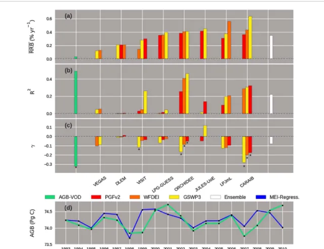
3.1. Global RRB and its sensitivity to ENSO
The GVM simulations show positive significant trends of global biomass, steeper than the observed one. Whereas the observedRRB = 0.03% yr−1, the ensem-ble of simulations shows RRB = 0.3%yr−1 (figure 1(a)) (hereafter RRB results are reported in units of % of change per unit of biomass per year). TheRRB in the individual simulations range between 0.1 (in VEGAS-WFDEI) and 0.6 (in CARAIB-VEGAS-WFDEI). In the case of VISIT, LPJmL and CARAIB, theRRB results strongly depend upon the climate forcing.
The inter-annual variability of biomass is con-trolled by annual RRB fluctuations. The observations and the ensemble mean are characterized by a tem-poral standard deviation of RRB of STD = 0.5 and STD = 0.2, respectively. The smallest STD equals 0.1 (ORCHIDEE-PGFv2) and the highest 0.9
(JULES-GSWP3) (table 3). The exceedingly large STD in JULES-GSWP3 results from a single strong RRB fluc-tuation around 2002. Amid the models, similar values ofSTD as in the observation are found for VEGAS-GSWP3 and CARAIB-WFDEI.
When looking at the sign changes of detrended RRB anomalies, the ensemble mean matches the observation in 11 out of 17 years. The best match between individual models and observation is found for VEGAS-GSWP3 (11 years) and the lowest one for DLEM-GSWP3 (6 years) (table3).
The results of the regression of global RRB with the Multivariate ENSO Index (MEI) (equation (3)) show the importance of ENSO events in explaining the inter-annual variability of global biomass (figure1(d)). The observed RRB to MEI regression shows a R2value of 0.5 (figure1(b)), as opposed to a model ensemble mean R2of 0.2. The highest valueR2= 0.5 in the simulations
corresponds to ORCHIDEE-WFDEI (table4). In the observations, the sensitivity of RRB to MEI (figure1(c)) (denoted by𝛾 and hereupon reported in the text in units of % yr−1per MEI unit change) is nega-tive and equals−0.32 ± 0.08. The ensemble mean does not show a significant sensitivity (at p-value≤ 0.05). However, significant negative sensitivities were iden-tified in VISIT-GSWP3 where 𝛾 = −0.12 ± 0.1, as well as in all the simulations of ORCHIDEE (from −0.05 ± 0.02 in PGFv2 to −0.17 ± 0.05 in GSWP3) and CARAIB (from−1.8 ± 0.7 in PGFv2 to −2.8 ± 1.1 in GSWP3). The intercept regression coefficients in the simulations can be practically assimilated toRRB (see figure S3 in SI).
After restricting the analysis to the Northern Hemisphere extra-tropical region (23◦N–85◦N), the observed RRB to MEI regression shows a negative sen-sitivity with𝛾 = −0.8 ± 0.2 and R2= 0.4 (see figure S4 in SI). In this region, the sensitivities of RRB in the GVM simulations are not significant (see figure S4 in SI). The opposite occurs in the Tropical region (23◦S— 23◦N), where the sensitivity of RRB is not significant in the observation (see figure S5 in SI), but in the simulations of VISIT-GSWP3 (−0.2 ± 0.1), JULES-PGFv2(−0.1 ± 0.03), CARAIB (from −0.3 ± 0.1 in WFDEI to−0.4 ± 0.1 in GSWP3) and of ORCHIDEE (from −0.05 ± 0.02 in PGFv2 to −0.2 ± 0.06 in GSWP3). The simulation CARAIB-PGFv2 shows the highest R2(0.5).
3.2. The regional RRB and underlying differences in NPP and RLB in the global vegetation models.
To gain understanding on the discrepancies in global biomass change, between the GVM simulations and the observation (figure 1(a)), the RRB analysis was applied to regions of natural forest with high biomass densities, namely the tropical forests of Amazonia (AMA) and Congo (CON) and the boreal forests of Western Siberia (WES), Central-Siberia (CES) and North-Western America (NWA)–the latter including
Figure 1. Global RRB derived from AGB-VOD and the global vegetation models and their relation to ENSO (described by the MEI) for the historical period 1993–2010. (a) The temporal mean of global RRB; (b) R2values of the RRB to MEI; (c) the RRB to MEI sensitivity parameter (∗ significant sensitivity (𝑝 ≤ 0.05)); (d) trajectory of global AGB-VOD (green) and its reconstruction using the results of the regression with MEI and the connection between RRB (equation (3)) (blue). The parameter values derived from AGB-VOD in green and the model ensemble mean of these quantities in white. Models: VEGAS, DLEM, VISIT, LPJ-GUESS, ORCHIDEE, LPJmL JULES, CARAIB. Climate forcings: PGFv2 (red), GSWP3 (orange) and WFDEI (yellow).
also temperate forest (figure 2 and table S1 in SI). Altogether, the contributions of these regions sum up ca. 40% of the total AGB considered in the global analysis.
The observation shows a major increase of biomass in WES (19% growth of AGB with respect to the beginning of the study period), that is characterized by RRB = 0.8 (figure 3(a)). This increment largely surpasses in magnitude the loss of biomass observed in NWA (RRB = −0.08), CES (RRB = −0.07), AMA (RRB = −0.07) and CON (RRB = −0.01). With the exception of CON, the decremental trends of biomass associated to the observed regional values of RRB are significant. In contrast, the RRB shown by the ensemble mean of the simulations is positive in all of the regions. According to the ensemble mean, the most intense growth of biomass occurs in CES (RRB = 0.8), followed by WES (RRB = 0.6), NWA (RRB = 0.4), CON (RRB = 0.2) and AMA (RRB = 0.2). The overestimation of biomass growth in the sim-ulations is also expressed as an underestimation of the fraction fA of the total area whereRRB < 0 (see section2.2.5). The least underestimation of this frac-tion in the boreal regions is found in NWA (ensemble mean: 32.4%; observation: 56.3%) and in the tropical
regions in CON (ensemble mean: 27.3%; observation: 61.7%) (see summary in tables S2-S6 in SI).
The individual simulations show positive values of RRB in all of the regions, excerpt for LPJmL-PGFv2, VEGAS (forced by GSWP3 and WFDEI) and VISIT (GSWP3 and WFDEI) in CON (figure3). Practically all of the trends of biomass associated to theRRB val-ues in the simulations are significant across the regions. The simulated increments of biomass show their best mutual agreement in AMA, with RRB ranging between 0.06 (VEGAS-WFDEI) and 0.3 (JULES-GSWP3). On the contrary, the largest inter-simulation discrepancies inRRB take place in CON, with values ranging from −0.4 (VISIT-WFDEI) to 1.4 (LPJmL-WFDEI). In the boreal regions, the largest spread of RRB occurs in CES, with values ranging between 0.1 (VEGAS-GSWP3) and 1.4 (LPJmL-GSWP2). In WES, RRB ranges from 0.3 (CARAIB-WFDEI) to 1.4 (ORCHIDEE-GSWP3) and in NWA from 0.08 (DLEM-PGFv2) to 0.9 (CARAIB-GSWP3) (see summary ofRRB results in tables S2–S6 in SI).
In those simulations showing the largest values of regional RRB, RRB is positive in at least 14 out of the 17 years covered by the study period. We remind that positive values of RRB occur whenever TRB, i.e.
Table 3. Summary statistics of the analysis of global RRB.
Observation/Model RRB(10−3yr−1) STD(10−3yr−1) Fraction of years where the sign of detrended RRB agrees with the sign of RRB derived from VOD
VOD 0.4 4.6 VEGAS GSWP3 1.3 4.5 0.7 WFDEI 1.2 4.3 0.5 VISIT PGFv2 3.0 2.0 0.6 GSWP3 1.4 2.1 0.5 WFDEI 2.8 2.3 0.6 DLEM PGFv2 2.1 2.0 0.4 GSWP3 2.1 2.1 0.4 WFDEI 2.1 2.3 0.4 LPJ-GUESS PGFv2 3.5 3.0 0.5 GSWP3 3.6 3.3 0.5 WFDEI 4.0 3.3 0.6 ORCHIDEE PGFv2 3.8 1.0 0.6 GSWP3 4.1 1.3 0.4 WFDEI 4.1 2.4 0.5 LPJmL PGFv2 3.1 3.1 0.6 GSWP3 5.6 2.7 0.6 WFDEI 3.7 2.9 0.7 JULES-UoE PGFv2 4.2 1.3 0.5 GSWP3 4.5 9.4 0.5 CARAIB PGFv2 3.6 3.0 0.4 GSWP3 4.3 5.0 0.5 WFDEI 6.3 3.7 0.5 ENSEMBLE 3.4 1.8 0.7
Figure 2. Map of temporal mean of RRB derived from annual biomass observations from Liu et al (2015) over the historical period 1993–2010. Blue boxes enclose the analyzed regions in Amazonia (AMA), Congo (CON), western Siberia (WES), Central Siberia (CES) and north-western America (NWA). Non-available and masked values (where the cover of farmland and pastures exceeds the 5% threshold of the grid-cell) are shown in gray.
the ratio NPP/B, exceeds RLB (equation (5)). The sim-ulations show strong TRB to NPP correlations (with a
R2above 0.7 (0.8) in 100 (86) of the 110 cases com-prised by the simulations across the regions). In all
the regions the significant trends of NPP are posi-tive (figure4) (NPP trends are hereafter denoted as TNPP and reported in units of Tg C yr−2; significant refers to 𝑝 ≤ 0.05)). Most of the simulations show
Table 4. Summary of the global RRB to MEI regression analysis (∗𝑝 ≤ 0.05). Observation/Model 𝛾(10−3yr−1) 𝛽(10−3yr−1) R2 P-value VOD −3.3 ± 0.8 0.7 0.5 2 × 10⁻³ VEGAS WFDEI −1.0 ± 1.1 1.4 0.0 0.4 GSWP3 −0.9 ± 1.1 1.3 0.0 0.4 VISIT PGFv2 −0.3 ± 0.5 3 0.0 0.5 WFDEI −0.5 ± 0.5∗ 1.5 0.1 0.4 GSWP3 −1.2 ± 0.5 2.9 0.3 0.04 DLEM PGFv2 0.1± 0.4 2.1 0.0 0.8 WFDEI −0.1 ± 0.5 2.1 0.0 0.9 GSWP3 −0.1 ± 0.4 2.1 0.0 0.8 LPJ-GUESS PGFv2 −0.4 ± 0.8 3.6 0.0 0.7 WFDEI −0.3 ± 0.8 3.6 0.0 0.8 GSWP3 −0.7 ± 0.8 4.1 0.0 0.4 ORCHIDEE PGFv2 −0.5 ± 0.2∗ 3.9 0.3 0.04 WFDEI −0.9 ± 0.3∗ 4.2 0.4 6 × 10⁻³ GSWP3 −1.7 ± 0.5∗ 4.3 0.5 3 × 10⁻³ LPJmL PGFv2 −1.0 ± 0.8 3.2 0.1 0.2 WFDEI −1.2 ± 0.6 5.8 0.2 0.07 GSWP3 −1.3 ± 0.7 3.9 0.2 0.08 JULES-UoE PGFv2 −0.5 ± 0.3 4.2 0.1 0.1 GSWP3 1.2± 2.4 4.4 0.0 0.7 CARAIB PGFv2 −1.8 ± 0.7∗ 3.8 0.3 0.02 WFDEI −2.0 ± 0.8∗ 4.6 0.0 0.02 GSWP3 −2.8 ± 1.1∗ 6.7 0.3 0.02 ENSEMBLE −0.8 ± 0.4 3.5 0.2 0.06
significant TNPPs in CES, with slopes rang-ing from 2.2± 0.8 (CARAIB-GSWP3) to 10.9 ± 2.2 (ORCHIDEE-WFDEI). In WES and NWA, signifi-cant TNPPs are shown only by the simulations of ORCHIDEE. In WES, these trends range from 1.7± 0.5 (GSWP3) to 2.6± 0.5 (WFDEI) and in NWA from 1.5± 0.7 (GSWP3) to 1.8 ± 0.6 (WFDEI). In the tropical regions, significant TNPPs occur mostly in CON, in all of the simulations forced by PGFv2, in DLEM, LPJmL, ORCHIDEE and LPJ-GUESS forced by GSWP3, as well as in DLEM-WFDEI. The lowest significant TNPP in CON equals 1.2± 0.5 (ORCHIDEE-GSWP3) and the highest one 6.7± 1.3 ( LPJmL-PGFv2). In AMA, significant TNPPs are dis-played only by DLEM, in the range between 2.2± 0.9 (PGFv2) and 3.6± 1.2 (WFDEI).
Hence, only in the case of ORCHIDEE-GSWP3 in WES the highest regional RRB coincides with a significant positive TNPP. In CES, the highest RRB is associated with a negative significant trend in RLB (−0.16% yr−2, in LPJmL-GSWP3) (figure4)
(RLB trends are subsequently denoted as TRLB and reported in units of % yr−2). Similarly in CON, the highest RRB is associated to a negative significant TRLB (−0.095, in LPJmL-WFDEI). Other cases where
biomass growth appears reinforced by negative sig-nificant TRLBs are: in WES, LPJmL-WFDEI (−0.05); in NWA, ORCHIDEE-WFDEI (−0.1) and the simu-lations of LPJmL (−0.08) and VISIT (−0.05) forced by PGFv2; in CON, in LPJ-GUESS-PGFv2 (−0.026), LPJ-GUESS-WFDEI (−0.03) and CARAIB-GSWP3 (−0.08). On the other hand, the increment of biomass is attenuated by positive significant TRLBs in CES, in all the simulations of VISIT (0.06–0.07) and ORCHIDEE (0.2–0.3); in WES, in VISIT-WFDEI (0.03); in CON, in VISIT-WFDEI (0.02) and in all the simulations of DLEM (0.004–0.006). Finally, in AMA, the positive significant TRLBs occur in DLEM (0.003, with forc-ings GSWP3 and WFDEI) and in LPJmL-PGFv2 (0.09) (summary of regional trends of NPP and RLB in tables S2–S6 in SI).
In the absence of significant TNPPs and TRLBs, as is the case of most of the simulations in NWA, differences inRRB could be simply interpreted as dis-crepancies at the level of the background simulated values of TRB (NPP) and RLB during the histori-cal period. However, important changes in biomass also occur during shorter subintervals. The negative RRB values (figure 3) in CON, in the simulations of VEGAS, are mainly due to an overall decrease in
Figure 3. Regional mean of RRB derived from AGB-VOD and the GVM simulations in the historical period 1993–2010 (here, ∗ indicates that the trends of biomass/AGB are significant (𝑝 ≤ 0.05)). Models: VEGAS, DLEM, VISIT, LPJ-GUESS, ORCHIDEE, LPJmL, JULES, CARAIB. Climate forcings: PGFv2 (red), GSWP3 (orange) and WFDEI (yellow). Color coding of forcing datasets as in figure1.
TRB values within the periods 1995–1998 and 2003– 2005, that co-occur along with important increments in RLB (see plots of regional trajectories of TRB and RLB in figures S6-S10 in SI). Similarly, the decrease of biomass described by LPJmL-PGFv2 in CON is mainly due to a sharp rise in RLB between 1994 and 1996, after which RLB remains above TRB until 2002. On the other hand, we notice that the high standard devi-ation of global RRB in JULES-GSWP3 (cf section 3.1) is related to large RLB variations occurring in CON, AMA and NWA, between years 2001 and 2004. Overall, in each region the simulations generated by different models and forcings show dissimilar trajec-tories of RLB and TRB. In spite of this, we notice that in AMA all the simulations describe a decrease in TRB between 1996–1998, followed by recovery until 1999.
These findings point to important differences regarding the relative influence of NPP (via TRB) and RLB on RRB (section2.2.4). Altogether, in most of the simulations the annual variations in regional RRB are mostly influenced by NPP (see figure S11 in SI). Particular cases where the influence of RLB on RRB is dominant are: in WES, CES and NWA, the simula-tions of VEGAS, LPJ-GUESS and CARAIB; in AMA, in the simulations of VEGAS, LPJ-GUESS (forced by WFDEI and GSWP3), CARAIB (GSWP3 and PGFv2), JULES-GSWP3 and LPJmL-PGFv2 and, in CON, LPJ-GUESS, LPJmL-WFDEI and CARAIB-GSWP3. Finally, the influences of NPP and RLB are closely comparable in the simulations LPJ-GUESS-WFDEI in CES, CARAIB-PGFv2 in WES, JULES-GSWP3 in CON and CARAIB-WFDEI in AMA.
Figure 4. Regional trends of NPP and RLB in the GVM simulations and their ensemble mean (white) in the historical period 1993– 2010 (∗significant trends (𝑝 ≤ 0.05)). Trends reported in terms of the percentage with respect to initial values at the beginning of the historical period. Models: VEGAS, DLEM, VISIT, LPJ-GUESS, ORCHIDEE, LPJmL, JULES, CARAIB. Climate forcings: PGFv2 (red), GSWP3 (orange) and WFDEI (yellow).
4. Discussion
4.1. The RRB concept, its interpretation and caveats
The main objective of this work is to analyze the abil-ity of the GVMs to reproduce historical changes in biomass. Evaluating the physiological component of biomass changes is important as a preliminary step towards assessing the model representations of direct anthropogenic influences. Consequently, this study focused on natural terrestrial ecosystems.
We used the AGB maps provided in Liu et al (2015) as observational reference to verify the trends and inter-annual variability of biomass. Other similar datasets are available (cf Saatchi et al 2011), but the Liu et al (2015) dataset is the only product provid-ing multi-year coverage. Since the GVMs do not report explicitly AGB but only total biomass, their comparison with observations can be achieved based on a relative metric (e.g. percentage change of biomass with respect to a baseline value). The underlying assumption of this approach is that the AGB to BGB ratio is constant in space and time (see explanation in S1.3 in SI). A lin-ear AGB to BGB relation has been shown to be a valid approximation for non-woody plants (Niklas 2005), forest ecosystems (Yang and Luo2011), as well as for aggregate biomass estimates involving different plant
communities (Cheng et al2015). The use of a rela-tive metric has the additional advantage of enabling the comparison of the intensity of changes in biomass across different ecosystems.
Moreover, we choose the RRB metric because: (i) biomass trajectories are determined by the exponential of the cumulative sum of RRB over time (see equa-tion (2) in the text and section S1.4 in SI). This is relevant since a persistent bias of RRB in the models, with respect to observations, may imply a non-linear increase in the error of biomass trajectories in long term projections (see illustration in figure S2 in SI); (ii) RRB equals the deviation of the actual turnover rate of biomass RLB from its equilibrium value TRB (equation (5)). Gaining knowledge on the dynam-ics and climate sensitivity of the turnover rate of biomass is critical to understand possible future tra-jectories for the terrestrial carbon cycle (Bloom et al 2016). For instance, the behavior of RLB has been recognized as a substantial source of uncertainty in multi-model projections of biomass in a similar set of GVMs (Friend et al2014). Moreover, a recent anal-ysis of boreal forests by Thurner et al (2017) has shown that an underestimation of the average of TRB leads to important discrepancies in biomass between observation and simulations.
Recently, Luo et al (2017) introduced a new framework to analyze the transient dynamics of car-bon pools in ecosystems from a systems perspective. In their formulation, changes in the ecosystem carbon storage are described by the carbon storage potential: the difference between the actual carbon storage and the carbon storage capacity (Olson1963). The latter being defined as the maximum amount of carbon that an ecosystem can store, given the environmental condition at a point in time. Under stationary envi-ronmental conditions, the transient dynamics of the carbon pools is determined by the decrease of the car-bon storage potential towards zero. The RRB bears similarity with the carbon storage potential concept. In absence of trends in environmental conditions, the biomass pool attains stationarity through the gradual balancing of RLB and TRB, occurring via the uptake and the loss of carbon.
Different factors may affect the reliability of the approach followed in this study to evaluate historical changes of biomass in the selected GVMs. For instance, intense drought episodes may compromise the consis-tency of the RRB comparison, between observed AGB and simulated total biomass, due to changes in car-bon allocation patterns in vegetation (Doughty et al 2015). However, the AGB product in Liu et al (2015) also embodies significant uncertainties, that are partly related to the spatial extrapolation method (Mitchard et al2014) based on Saatchi et al (2011). Moreover, this AGB dataset may be of limited use for evaluating impacts of climate extremes on tropi-cal forests, in view of the possible underestimation of inter-annual variations of biomass by VOD signals, in comparison with other satellite indicators of vegeta-tion (Liu et al2011). In addition, we notice that the AGB time-series indicate a decrease of biomass in arid regions of Australia (figure 2), which still has to be confirmed by other techniques. It is also important to bear in mind the limitations of the land-mask applied to disentangle the anthropogenic and physiologic com-ponents of RRB. The land cover selection criterion applied for the regional analysis was especially strict, in the sense that only grid cells with a classification of 100% natural vegetation were considered (see com-parison of surface areas in table S1 in SI). However, the land-cover classification was based on the available information from year 2005 and important changes in land-cover have occurred ever since Houghton
et al (2012). Finally, the construction of the mask did not accounted for information on other human activi-ties, such as wood harvest in managed and unmanaged forests, regrowth in abandoned agricultural areas (Pan et al 2011), or landscape fragmentation (P¨utz
et al2014).
4.2. Global aspects of RRB
The global observed RRB indicates an increase in global biomass between 1994 and 2010 (figure1(a)). As reported by Zhu et al (2016), recent increments of
global biomass have been attributed to positive plant-physiological effects of increasing atmospheric CO2, as well as to the prolongation of growing seasons in the Northern Hemisphere, as a result of global warm-ing. The global increase of biomass described by the GVMs appears too optimistic, with the ensemble mean of the simulations showing a globalRRB one order of magnitude larger than the observed one (figure1(a)).
The sensitivity of the global RRB variations to ENSO in the observation (figure 1(c)) is practically explained by the response of AGB in the Northern Hemisphere extra-tropic (see figure S4 in SI). The apparent absence of a significant ENSO sensitivity in the observation of RRB in the tropics (see figure S5 in SI) is striking, as it contrasts with evidence on the strong influence of El Nĩno events, on extreme heat and drought conditions, over the Amazonia forests (Jim´enez-Mũnoz et al2016). This ambiguity suggests a limited capacity of VOD signals to adequately capture inter-annual variations of AGB in tropical forests. On the contrary, the simulations of 4 out of the 7 GVMs show significant sensitivities of RRB in the tropics (see figure S5 in SI), but none of them in the Northern Hemisphere (see figure S4 in SI). The underlying differ-ences in RRB variations in the simulations are discussed in further detail below in section4.3.
4.3. Regional aspects of RRB
The regional value ofRRB in WES is higher in the observation than in most of the simulations (figure3). In the rest of the boreal regions analyzed, the sign of RRB is negative in the observation, and positive in all of the simulations. A similar situation is found for AMA. The analysis of RRB in CON shows no significant change of biomass in the observation, but increments in most of the simulations. These findings are rele-vant for the purpose of understanding the difference between the observed and simulated trends of global biomass (figure1(a)), given the broad extent and high concentration of biomass in these regions (whose con-tributions sum up to ca. 40% of the global total AGB in this analysis).
The overestimation of the regional RRB in the simulations may be related to the CO2sensitivity of carbon uptake. All of the regional significant TNPPs simulated by the GVMs are positive (figure 4). The significant TNPPs in the boreal regions are mostly local-ized in CES, whereas in the tropics these mainly occur in CON. A recent analysis of the CMIP5 earth system models, forced only by the increase of CO2(Smith et al 2016) over the period 1982–2011, has pointed to an overestimation of incremental NPP trends. The exces-sive CO2response of NPP was attributed to the lack of nutrient constraints in most of the CMIP5 mod-els. This possibility could be debated in the case of the GVMs used here, where the degree of overesti-mation of trends of gross primary productivity (GPP) depends on the observational reference that is used as benchmark (Ito et al2017). Although the presence
of an excessive CO2 fertilization effect in all of the GVM simulations cannot be excluded, its role in explaining differences inRRB is not conclusive. Nitro-gen limitation is included in VEGAS, DLEM and LPJ-GUESS (table1) and the significant TNPPs dis-played by VEGAS and LPJ-GUESS in CES are below the ensemble mean (figure 4). However, the RRB values shown by the LPJ-GUESS simulations in this region (figure3) are comparably high as those shown by the models where an excess in CO2 fertilization could be expected (due to their lacking representation of nitrogen limitation). Overall, we find that the single case where the largest regional value ofRRB coincides with a positive significant TNPP corresponds to the simulation ORCHIDEE-GSWP3 in WES (see figures 3and4). Indeed, regardless how disproportionate the CO2response of simulated NPP may be, we recall that an increase of NPP at a point in time will lead to a greater increment of biomass provided it raises further the value of TRB above RLB (equation (5)). In other words, understanding discrepancies in biomass growth necessarily requires to assess NPP (or more specifically TRB) and RLB simultaneously.
In the Boreal regions, the variations of RRB are mainly influenced by RLB in the simulations of VEGAS, LPJ-GUESS and CARAIB, and are dominated by NPP (via TRB) in the rest of the models (see fig-ure S11 in SI). The simulations do not reproduce the observed significant ENSO sensitivity of RRB in the Northern Hemisphere extra-tropics. The analysis of boreal regions by Thurner et al (2017) pointed out the failure of a very similar set of GVMs at repro-ducing phenomenological relations between climate variables and average TRB. Amidst the physiological processes involved in the turnover of biomass, mor-tality is highly complex, not thoroughly understood and, consequently, insufficiently described in global vegetation models (Steinkamp and Hickler2015). In addition to the responses of TRB and RLB to climate and CO2concentrations, disturbances can constitute an important source of differences in biomass change. During the historical period covered by the RRB anal-ysis, decrements of biomass occurred in NWA as a result of widespread and severe pine beetle outbreaks (Kurz et al2008). The positiveRRB values shown by the simulations in NWA may thus be attributed to the lack of representation of insect infestation effects in the GVMs. In CES, incremental trends of fire inten-sity and frequency were reported also for the analyzed period (Ponomarev et al2016, Schaphoff et al2016). Consequently, significant increments of RLB in CES could be expected in the simulations of those mod-els featuring fires, i.e. CARAIB, LPJmL, LPJ-GUESS, VISIT and VEGAS (table2). Among them, the sim-ulations of CARAIB show a high fraction of the total area of CES withRRB < 0, as in the observation (see table S5 in SI). However, significant positive TRLBs in CES are shown only by VISIT and ORCHIDEE (figure 4). Given the time average of TRB displayed by VISIT
and ORCHIDEE in CES, an increase in the time aver-age of RLB by at most 3.8% and 6.5%, respectively, would be required to match the observedRRB in this region. It is important to mention that limitations of fire models in reproducing observed trends in burned area have been identified in a recent GVM intercompar-ison (Andela et al2017). In WES, the drastic increase of the observed carbon sink can be partly attributed to the expansion of forested areas, following agricul-tural abandonment and reduced harvesting (Zhu et al 2016). The generally lowerRRB values shown by the simulations in this region, compared to the observa-tion, could be explained by the lack of representation of these processes in the models (or equivalently, by the failure of the land-mask applied to exclude their influ-ence from the RRB analysis). Nonetheless, the case of WES illustrates the importance of analyzing the spatial aspects of the NPP and RLB trends, as the observa-tion also shows a decline of biomass over ca. 32% of the total area (see table S3) –occurring mainly in the North-Eastern part of this region (figure2). We find that comparable area fractions in WES, as in the observation, are displayed by LPJmL-PGFv2 (32.7%) and CARAIB-GSWP3 (34.6%), whereas those shown in the rest of the simulations are lower. Overall, these findings suggest that further analysis of differences in average TRB (NPP) and RLB, as well as of the imple-mentation of fire dynamics and disturbances in the GVMs is required.
In the case of tropical forests, the approach followed in this study may not be reliable to verify the behavior of RRB in the GVMs. The positive sign of RRB in the simulations of AMA is in qualitative agree-ment with previous observations of biomass change in intact forest (Pan et al 2011). However, recent analyses of in-situ data of Amazonia have shown a significant positive trend in mortality during the last decades (Brienen et al2015) and subsequent biomass loss and carbon release after droughts in 2005 and 2010 (Lewis et al2011). The role of drought as a driver of tree mortality is corroborated by experimental results in this region (Rowland et al2015, Feldpausch et al 2016). Yet the analysis of Brienen et al (2015) asserts that, in spite of the impact of severe droughts, mature forests in Amazonia remained accumulating biomass during the 1983–2010 period. In this view, in addition to droughts, the negative sign of the AGB deriva-tion of RRB in AMA can be related to the impacts of human activities, such as clearing, landscape frag-mentation and selective logging (Morton et al2011, Houghton et al 2012) –not being excluded by the land-mask. A similar situation holds for the CON region, which has also experienced degradation (Zhu-ravleva et al2013). Moreover, the presence of intense droughts in Amazonia may cast doubts on the validity of the AGB-to-BGB isometry over time, due to changes in carbon allocation patterns in vegetation (Doughty
et al 2015). Moreover, the AGB product in Liu
extremes related to ENSO on biomass variations in tropical forests.
The GVM simulations show the best mutual agree-ment inRRB in AMA, compared to the rest of the regions. On the contrary, the largest spread of simu-latedRRB occurs in CON. The positive and negative extreme values ofRRB in CON are associated, respec-tively, with negative and positive significant TRLBs. In relation to the ENSO sensitivities of RRB exhibited by some of the simulations in the tropics (see fig-ure S5 in SI), the analysis of AMA and CON shows that RRB variations are mostly influenced by NPP in JULES-PGFv2, VISIT-GSWP3, ORCHIDEE-GSWP3; whereas these are dominated by RLB in CARAIB-GSWP3. Altogether, in models where the description of mortality and/or leaf turnover is directly modulated by climate (see table2), the degree of influence of RLB on RRB varies across regions and climate forcings (see figure S11 in SI). Conversely, in VISIT and DLEM, where the turnover of biomass is simply modulated by one factor (fire and tree age, respectively), the varia-tions of RRB are consistently dominated by NPP. In spite of these differences, in AMA all of the simulations show a drop of NPP between 1996 and 1998, that leads to a decrease in TRB (see figure S7 in SI). This can be interpreted as a response to the extreme El Nĩno event that occurred during this period. For further informa-tion on the response of the carbon uptake to climate variations in the GVMs analyzed here we refer to Ito
et al (2017), Chang et al (2017). Finally, the RRB results at the global (figure1(a)) and regional (figure2) scales are in general sensitive to the climate forcing dataset. This can be partly attributed to differences in the car-bon uptake flux induced by the discrepancy in solar radiation among the forcing datasets (Ito et al2017).
5. Conclusions
The historical changes of biomass in natural terrestrial ecosystems described by the simulations of an ensem-ble of eight GVMs was evaluated against time-series of AGB, reconstructed from the signals of Vegeta-tion Optical Depth retrieved from satellite passive microwave sensors over the period 1993–2010. For this purpose, the model output and the AGB observation were compared in terms of the relative rate of change of biomass RRB. In particular, the study focused on: the temporal mean and standard deviation of global RRB and its relation to ENSO events, as well as on the regional aspects of the temporal mean and annual vari-ations of RRB, in relation to changes in NPP and RLB. The main findings of the analysis are: (a) the temporal mean of RRB in the models is one order of magni-tude higher than in the observed AGB records; (b) the observed RRB shows a significant sensitivity of AGB in the Northern Hemisphere to ENSO events, but not in the tropics; (c) on the contrary, some of the GVMs show a significant sensitivity of RRB to ENSO in the tropics,
while none of them reproduces the observed sensitivity in the Northern Hemisphere; (d) in most of the models the annual variations of RRB are mostly influenced by NPP, in comparison to RLB. Overall, these findings underline the importance of conducting a further detailed analysis of both RLB and its equilibrium coun-terpart TRB and more specifically on their background values and sources of variation, including the effect of CO2, climate extremes and disturbances. In turn, this may require improving our current capacity to accurately quantify annual changes in biomass and NPP. In addition, a detailed and updated land-cover classification is necessary to effectively disentangle the physiological and anthropogenic components of TRB and RLB.
Acknowledgments
This work has been carried under the framework of the Inter-Sectoral Impact Model Intercomparison Project Phase 2a (ISIMIP2a) funded by the Ger-man Federal Ministry of Education and Research (BMBF, grant no. 01LS1201A1). The work of A Garc´ıa Cant́u was supported by the European Union Seventh Framework Programme FP7/2007–2013 under grant agreement n◦603864 (HELIX). In addition, the work was supported within the framework of the Leibniz Competition (SAW-2013 P IK-5). A Garc´ıa Cant́u also acknowledges J Schewe and J Salgado for atten-tive proofreading and suggestions on the manuscript, as well as Professor G Nicolis from the Free Uni-versity of Brussels (ULB) for important remarks and for pointing to interesting references on model pre-dictability. H Tian, S Pan and J Yang acknowledge support by US National Science Foundation Grants (AGS1243232, CNH1210360). A Ito and K Nishina acknowledge support by the Ministry of Environ-ment, Japan (Environmental Research and Technology Development Fund S-10).
ORCID iDs
Anselmo Garc´ıa Cant́u https://orcid.org/0000-0001-6020-6324
Fang Zhao https://orcid.org/0000-0002-4819-3724 Sebastian Ostberg https://orcid.org/0000-0002-2368-7015
References
Andela N et al 2017 A human-driven decline in global urban area
Science356 1356–62
Best M et al 2011 The joint UK land environment simulator (JULES), model description–Part 1: energy and water fluxes
Geosci. Model Dev.4 677–99
Bloom A, Exbrayat J, van der Velde I, Feng L and Williams M 2016 The decadal state of the terrestrial carbon cycle: global retrievals of terrestrial carbon allocation, pools, and residence time Proc. Natl Acad. Sci.113 1285–90
Bondeau A et al 2007 Modelling the role of agriculture for the 20th century global terrestrial carbon balance Glob. Change Biol. 13 679–70
Brienen R et al 2015 Long-term decline of the Amazon carbon sink
Nature519 344–8
Chang J et al 2017 Benchmarking carbon fluxes of the ISIMIP2a biome models Environ. Res. Lett.12 045002
Chen M et al 2017 Regional contribution to variability and trends of global gross primary productivity Environ. Res. Lett. 12 105005
Cheng D, Zhong Q, Niklas K, Ma Y, Yang Y and Zhang J 2015 Isometric scaling of above- and below-ground biomass at the individual and community levels in the understorey of a sub-tropical forest Ann. Bot.115 303–13
Clark D et al 2011 The joint UK land environment simulator (JULES), model description–Part 2: carbon fluxes and vegetation dynamics Geosci. Model Dev.4 701–22
Doughty C et al 2015 Drought impact on forest carbon dynamics and fluxes in Amazonia Nature519 78–82
Dury M, Hambuckers A, Warnant P, Henrot A, Favre E, Ouberdous M and Franc¸ois L 2011 Responses of European forest ecosystems to 21st century climate: assessing changes in interannual variability and fire intensity iForest-Biogeosci.
Forest.4 82
Erb K, Fetzel T, Plutzar C, Kastner T, Lauk C, Mayer A, Niedertscheider M, K¨orner C and Haberl H 2016 Biomass turnover time in terrestrial ecosystems Nat. Geosci. 9 674–8 Feldpausch T et al 2016 Amazon forest response to repeated
droughts Glob. Biogeochem. Cycles 30 964–98
Friend A et al 2014 Carbon residence time dominates uncertainty in terrestrial vegetation responses to future climate and atmospheric CO2Proc. Natl Acad. Sci. 111 3280–85
G´erard J, Nemry B, Francois L and Warnant P 1999 The interannual change of atmospheric CO2: contribution of subtropical ecosystems? Geophys. Res. Lett.26 243–46
Goldewijk K, Beusen A, van Drecht G and de Vos M 2011 The HYDE 3.1 spatially explicit database of human-induced global land-use change over the past 12 000 years Glob. Ecol.
Biogeogr.20 73–86
Harper A et al 2016 Improved representation of plant functional types and physiology in the joint UK land environment simulator (JULES v4.2) using plant trait information Geosci.
Model Dev.9 2415–40
Huntzinger D, Schwalm C, Michalak A, Schaefer K, King A, Wei Y, Jacobson A, Liu S, Cook R and Post W 2013 The North American carbon program multi-scale synthesis and terrestrial model intercomparison project– Part 1: overview and experimental design Geosci. Model Dev.6 2121–33
Houghton R, House J, Pongratz J, van der Werf G, DeFries R, Hansen M, Le Qu´er´e C and Ramankutty N 2012 Carbon emissions from land use and land-cover change Biogeosciences 9 5125–42
Ito A and Inatomi M 2012 Water-use efficiency of the terrestrial biosphere: a model analysis focusing on interactions between the global carbon and water J. Hydrometeorol.13 681–94
Ito A et al 2017 Photosynthetic productivity and its efficiencies in ISIMIP2a biome models: benchmarking for impact assessment studies Environ. Res. Lett. 12 085001
Jim´enez-Mũnoz J C, Mattar C, Barichivich J, Santamar´ıa-Artigas A, Takahashi K, Malhi Y, Sobrino J and van der Schrier G 2016 Record-breaking warming and extreme drought in the Amazon rainforest during the course of El Nĩno 2015–2016
Sci. Rep.6 33130
Keeling C and Whorf T 2005 Atmospheric CO2records from sites in the SIO sampling network Trends: A Compendium of Data
on Global Change (Oak Ridge, TN: Carbon Dioxide
Information Analysis Center, Oak Ridge National Laboratory, US Department of Energy)
Krinner G et al 2005 A dynamic global vegetation model for studies of the coupled atmosphere-biosphere system Glob.
Biogeochem. Cycles 19 1
Kurz W, Stintson G, Rampley J, Dymond C and Neilson T 2008 Risk of natural disturbances makes future contribution of
Canada’s forests to the global carbon cycle highly uncertain
Proc. Natl Acad. Sci.105 1551–55
Le Qu´er´e C et al 2015 Global carbon budget 2015 Earth Syst. Sci.
Data7 349–96
Lewis S, Brando P, Phillips O, van der Heijden G and Nepstad D 2011 The 2010 Amazon drought Science 331 554
Liu Y, de Jeu A, McCabe M, Evans J and van Dijk A 2011 Global long-term passive microwave satellite-based retrievals of vegetation depth Geophys. Res. Lett. 38 L18402
Liu Y et al 2015 Recent reversal in loss of global terrestrial biomass
Nat. Clim. Change 5 470–4
Luo Y et al 2017 Transient dynamics of terrestrial carbon storage: mathematical foundation and its applications Biogeosciences 14 145
Mitchard E et al 2014 Markedly divergent estimates of Amazon forest carbon density from ground plots and satellites Glob.
Ecol. Biogeogr.23 935–46
Morton D, Sales M, Souza C and Griscom B 2011 Historic emissions from deforestation and forest degradation in Mato Grosso, Brazil: 1) source data uncertainties Carbon Balance
Manage. 6 18
Niklas K 2005 Modelling below- and above-ground biomass for non-woody and woody plants Ann. Bot.95 315–21
Olson J 1963 Energy storage and the balance of producers and decomposers in ecological systems Ecology44
322–31
Pan Y et al 2011 A large and persistent carbon sink in the world’s forests Science333 988–93
Ponomarev E, Kharuk V and Ranson K 2016 Wildfires dynamics in Siberian larch forests Forests 7 125
Portmann F, Siebert S and D¨oll P 2010 MIRCA2000—Global monthly irrigated and rainfed crop areas around the year 2000: A new high-resolution data set for agricultural and
hydrological modeling Glob. Biogeochem. Cycles24 1
P¨utz S et al 2014 Long-term carbon loss in Neotropical forests Nat.
Commun. 5 503
Ramankutty N, Evan A, Monfreda C and Foley J 2008 Farming the planet: 1. Geographic distribution of global agricultural lands in the year 2000 Glob. Biogeochem. Cycles 22 1
Rowland L et al 2015 Death from drought in tropical forests is triggered by hydraulics not carbon starvation Nature528 119–22
Saatchi S et al 2011 Benchmark map of forest carbon stocks in tropical regions across three continents Proc. Natl Acad. Sci.
USA 108 9899–904
Schaphoff S, Reyer C P O, Schepaschenko D, Gerten D and Shvidenko A 2016 Observed and projected climate change impacts on Russia’s forests and its carbon balance Forest Ecol.
Manage.361 432–44
Sitch S, Friedlingstein P, Gruber N, Jones S, Murray-Tortarolo G, Ahlstr¨om A, Doney S, Graven H, Heinze C and Huntingford C 2015 Recent trends and drivers of regional sources and sinks of carbon dioxide Biogeosciences 12 653–67
Smith B et al 2014 Implications of incorporating N cycling and N limitations on primary production in an individual-based dynamic vegetation model Biogeosciences 11 2027–54 Smith K et al 2016 Large divergence of satellite and Earth system
model estimates of global terrestrial CO2fertilization Nat.
Clim. Change6 306–10
Steinkamp J and Hickler T 2015 Is drought-induced forest dieback globally increasing? J. Ecol. 103 31–43
Thurner M et al 2017 Evaluation of climate-related carbon turnover processes in global vegetation models for boreal and temperate forests Glob. Change Biol.23 3076–3091
Tian H et al 2015 North American terrestrial CO2uptake largely offset by CH4 and N2O emissions: toward a full accounting of the greenhouse gas budget Clim. Change129 413–26
Warnant P, Francois L, Strivay D and Gerard J 1994 CARAIB: a global model of terrestrial biological productivity Glob.
Biogeochem. Cycles8 255–70
Wolter K and Timlin M 2011 El Nĩno/Southern Oscillation behaviour since 1871 as diagnosed in an extended multivariate ENSO index (MEI.ext) Intl. J. Climatol.31 1074–87
Yang Y and Luo Y 2011 Isometric biomass partitioning pattern in forest ecosystems: evidence from temporal observations during stand development J. Ecol. 99 431–7
Zeng N, Mariotti A and Wetzel P 2005 Terrestrial mechanisms of interannual CO2variability Glob. Biogeochem. Cycles 19 1
Zhu Z et al 2016 Greening of the Earth and its drivers Nat. Clim.
Change 6 791–5
Zhuravleva I, Turubanova S, Potapov P, Hansen M, Tyukavina A, Minnemeyer S, Laporte N, Goetz S, Verbelen F and Thies C 2013 Satellite-based primary forest degradation assessment in the Democratic Republic of the Congo, 2000–2010 Environ.