On the System Level Prediction of Joint Time Frequency Spreading Systems with Carrier Phase Noise

HAL Id: hal-00447397

https://hal.archives-ouvertes.fr/hal-00447397

Submitted on 14 Jan 2010

HAL is a multi-disciplinary open access archive for the deposit and dissemination of sci-entific research documents, whether they are pub-lished or not. The documents may come from teaching and research institutions in France or abroad, or from public or private research centers.

L’archive ouverte pluridisciplinaire HAL, est destinée au dépôt et à la diffusion de documents scientifiques de niveau recherche, publiés ou non, émanant des établissements d’enseignement et de recherche français ou étrangers, des laboratoires publics ou privés.

On the System Level Prediction of Joint Time

Frequency Spreading Systems with Carrier Phase Noise

Youssef Nasser, Mathieu Des Noes, Laurent Ros, Geneviève Jourdain

To cite this version:

Youssef Nasser, Mathieu Des Noes, Laurent Ros, Geneviève Jourdain. On the System Level Prediction of Joint Time Frequency Spreading Systems with Carrier Phase Noise. IEEE Transactions on Commu-nications, Institute of Electrical and Electronics Engineers, 2010, 58 (3), pp.839-850. �hal-00447397�

(†) This paper was been presented in part at the seventh IEEE International Workshop on Signal Processing Advances for Wireless Communications, IEEE SPAWC, Cannes France, July 2006.

(††) The paper has been submitted one month after the decease of Genevieve Jourdain.

On the System Level Prediction of Joint Time

Frequency Spreading Systems with Carrier Phase

Noise

(†)

Youssef Nasser(*), Mathieu des Noes(*), Laurent Ros(**) and Geneviève Jourdain(††)

(*)

youssef.nasser@cea.fr / mathieu.desnoes@cea.fr CEA-LETI, 38054 Grenoble cedex 09 France

(**) laurent.ros@gipsa-lab.inpg.fr, GIPSA-Lab, Domaine universitaire - BP 46- 38402 Saint Martin d'Hères cedex, France

Abstract--- Phase noise is a topic of theoretical and practical interest in electronic circuits. Although progress has been made in the characterization of its description, there are still considerable gaps in its effects especially on multi-carrier spreading systems. In this paper, we investigate the impact of a local oscillator phase noise on the multi-carrier 2 dimensional (2D) spreading systems based on a combination of orthogonal frequency division multiplexing (OFDM) and code division multiple access (CDMA) and known as OFDM-CDMA. The contribution of this paper is multifold. First, we use some properties of random matrix and free probability theory to give a simplified expression of signal to interference and noise ratio (SINR) obtained after equalization and despreading. This expression is independent of the actual value of the spreading codes and depends mainly on the complex amplitudes of estimated channel coefficients. Secondly, we use this expression to derive new weighting functions which are very interesting for the radio frequency (RF) engineers when they design the frequency synthesizer. Therefore, based on these asymptotic results, we adapt a new method to predict the bit error rate (BER) at the output of the channel decoder by using an effective SINR value. We show by simulations the validity of our models and that at a given BER, the required signal to noise ratio (SNR) may easily increase due to the carrier phase noise.

Index Terms--- Multi-carrier spreading systems, large system analysis, phase noise, SINR, EESM.

I. INTRODUCTION

Recently, orthogonal frequency and code division multiplexing (OFCDM) access technology has been investigated for the next generation of mobile communication systems [1][2]. It is a combination of orthogonal frequency division multiplexing (OFDM) and code division multiple access (CDMA). The interest of the 2D spreading systems known as OFDM-CDMA is to optimize the trade-off between diversity gain and multiple access interference (MAI).

To achieve high spectrum efficiency, OFDM-CDMA systems will implement a large number of sub-carriers and, as a consequence, will be highly sensitive to the carrier phase noise (CPN) [3]. The effect

2

of the CPN could be similar to that caused by a constant carrier frequency offset (CFO) i.e. CPN introduces a phase rotation on the received symbols and generates inter-carrier interference (ICI). However, in contrast to the CFO, the CPN is a random process and needs a whole apart study. In the literature, several works could be found on the CFO effects in the mutli-carrier based systems [3][4][5]. We will restrict our study in this paper to the CPN effects and results in OFDM-CDMA systems. In a multi-carrier transmission scheme like OFDM-CDMA, the CPN creates two effects: common phase error (CPE) and ICI. The CPE alters equivalently different carriers by causing sub-carrier phase rotation while ICI introduces interference to any sub-carrier from all other sub-carriers. In literature, the CPN effect has been presented in some papers for OFDM [3][6][7] and MC-CDMA systems [8]. Nevertheless, for MC-CDMA systems, the analytical results of [8] have assumed independent identically distributed (i.i.d.) spreading codes. Moreover, their results are only suitable for additive white Gaussian noise (AWGN) and small angle approximation of the CPN. In [9], the performance of OFDM-CDMA systems is derived in terms of signal to interference and noise ratio (SINR) degradation at the detector output and the channel coding is not accounted for. Moreover, a small angle approximation is assumed. To the authors’ knowledge, no contribution has been presented without the assumption of a small angle approximation.

In this paper, we propose a new approach to present the degradation caused by the CPN on the performance of the OFDM-CDMA systems. Our contribution extends the work of [9] which was done for a CPN in the MC-CDMA system. It is also based on our previous work done for different synchronization errors [10][11][12][13]. Contrarily to the previous works, we consider in this paper a CPN with small angle approximation but also with small variation approximation.

The contribution of our work can be summarized as follows.

1) Using some properties of random matrix (RM) and free probability (FP) theories, we develop a new analytical expression of the SINR in an asymptotic regime. This SINR formula is independent of the actual values of the spreading codes while taking into account their orthogonality. It depends only on the complex amplitudes of the channel coefficients, the average transmitted power of the interfering users and the affected power of the reference user.

2) Using asymptotic SINRs, we are able to derive SINR degradations and new weighting functions, such as proposed by Stott for OFDM system [6]. These functions will give a better understanding of the CPN effect on the system performance. Indeed, using these functions, we show that the low frequency components of the CPN power spectral density (PSD) have more impact on the ICI while high frequency components have more impact on the inter-band interference (IBI). As a consequence, using these functions, RF engineers will adapt easily the oscillator and the phase locked-loop (PLL) specifications [14].

3

3) Using asymptotic SINRs, we adapt a technique initially used in OFDM system to predict the bit error rate (BER) at the output of the channel decoder in the OFDM-CDMA systems. This technique, called exponential effective SNR mapping (EESM) [15][16] provides a reliable link between link level simulations and system level simulations. We show that the EESM technique is independent of the spreading system and of the CPN value. It depends only on the modulation and coding scheme (MCS). This article is organised as follows. Section II describes the transmission model of the OFDM-CDMA system including transmitter, channel model with CPN, and receiver. Section III gives an asymptotical expression of the estimated SINR. In section IV, we derive new weighting functions for the OFDM-CDMA systems while section V presents the system performance without channel coding. Section VI describes the EESM technique and its validation through simulations. Eventually, conclusions are drawn in section VII.

II. SYSTEM MODEL WITH CARRIER PHASE NOISE

Figure 1 shows a generalized framework of the 2D spreading OFDM-CDMA transmitter/receiver chain for a downlink communication with Nu users. For each user m, information bits bm are first

channel encoded with a convolutional encoder of coding rate R, randomly interleaved, and fed directly to a quadrature amplitude modulation (QAM) module which assigns B bits for each of the complex constellation points. Therefore, each complex symbol is spread by a Walsh-Hadamard (WH) sequence of Nc chips (Nu≤Nc), and scrambled by a portion of Nc chips of the cell specific long pseudo random

sequence. This scrambling code is used to minimize multi-cell interference. The resulting chips are then allocated on a time/frequency grid as shown in Figure 2. Assuming an IFFT of N sub-carriers, each user transmits S=N/NF data symbols am[s] of the mth user on the jth OFDM-CDMA block

composed of NT OFDM symbols. NF and NT are respectively the frequency and time domain spreading

factors. The system is thus a general case of the MC-CDMA [18] and MC-DS-CDMA [19] systems. The scheme is identical for other users using one specific WH sequence by user. For simplicity and without loss of generality, we will drop the index j in the sequel. The signal at the IFFT input is:

[

]

1

[ ]

, 0 [ ] 0,..., 1; 0,..., 1, 0,..., 1 u N q F m m m s T m T F d sN n P a s c nN q q N s S n N − = + = + = − = − = −

∑

(1)

In (1), dq[sNF+n] is the spread symbol of all users transmitted on the nth sub-carrier of the sth sub-band

during the qth OFDM symbol. Pm is the transmitted power allocated to the mth user’s signal and

assumed identical in all sub-bands, cm,s represents its spreading sequence.

At the output of the IFFT, a cyclic prefix (CP) of ν samples is inserted to discard the inter symbol interference (ISI). The signal is then converted to the transmit carrier frequency FTX by the RF unit and

4

passed thourgh a multipath channel described as a finite impulse response (FIR) filter

∑

− = − = 1 0 ] [ ) ( W k k q q z g k z

h whose hq(z) is the z transform. gq[k] is the channel impulse response (CIR) and W

is the delay spread which is assumed less than the cyclic prefix (W≤ν). The signal at the channel output is then corrupted by an AWGN with zero mean and variance equal to

σ

2. At the receiving side, the signal is down converted by the receiver RF unit using the receiver carrier frequency FRX.

In practice, carrier frequency oscillators are affected by phase noise. The term CPN is widely used to describe short term frequency fluctuations around the frequency f0 of the oscillator. In time domain, it

can be described as a continuous Brownian motion process with zero mean and a variance equal to 2Dt where D is the CPN line-width commonly known as diffusion factor [17] and t is the time variable. It characterizes the 3-dB bandwidth of its Lorentzian PSD function [3]. Due to filtering and modelling problems, we are generally interested to the medium frequency part of the CPN PSD [9][14]. Then, the CPN is characterised by independent Gaussian increments in time domain represented as a finite-power Wiener phase noise. In discrete time representation, it can be obtained at each time sample k as:

] [ ] [ ] 1 [k ε k ρ k ε + = + ₍₂₎

where ε[k]is the sampled CPN and ρ[ ]k is a white Gaussian random variable with zero mean and variance equal to 2DTs where Ts is the sampling period. Its PSD is given by:

2 2 ) 2 ( 2 ) ( f D D f S

π

ε = ₊ (3)

In order to reduce the frequency fluctuations, the oscillator is integrated in a PLL controlled by an ultra stable oscillator working at low frequency. Since the VCO operates at high frequency, the PLL implements a low pass filter FB(z) used in a closed-loop scenario. As a consequence, the VCO Wiener

phase noise is filtered by a high-pass filter F(z)=1- FB(z). At the output, the filtered phase noise PSD is:

2 2 ) ( ) ( ) (f S f F ej f S_θ = _ε π ₍₄₎

In this paper, the high-pass PLL synthesizer is modelled by a second order filter whose coefficients are synthesized according to the cut-off frequency and the resonance parameter. It is given by:

2 2 1 1 0 2 2 1 1 0 ) ( _{− −} − − + + + + = z a z a a z b z b b z F ₍₅₎

where a0, a1, a2, b0, b1, and b2 are the PLL filter coefficients.

Generally, the CPN occurs at the transmitter and receiver as a phase rotation around the respective carrier frequency. In this paper, both phase rotations of the CPN are superposed at the receiver. Their superposition can be represented by a random phase rotation of the samples at the input of the CP

5

remove module. After FFT demodulation, the signal carried by the (wNF+p)th sub-carrier of the qth

OFDM symbol can be written as [10]:

[

wN p

]

d

[

sN n

]

ws pnq N

[

wN p

]

R _{q F} S s N n F q F q F + + + = +

∑ ∑

− = − = 1 0 1 0 ) , , , , ( φ (6)

w is the desired sub-band index (w = 0,…, S-1) and p is the index of a sub-carrier in the wth sub-band (p= 0,…, NF-1).

φ

(w,s,p,n,q) is the equivalent channel transfer function including IFFT, CIR, FFT and

CPN. It is given by:

(

)

∑

− =       _{− + −} − + = 1 0 ] [ exp ) ( ) ( 2 exp ] [ ) , , , , ( N u q F F q u j u N n p N s w j N n sN h q n p s w

π

θ

φ

(7)

Equation (7) shows that for w=s and p=n,

φ

(w,w,p,p,q) characterizes the CPE altering in an equivalent manner the signal transmitted on each sub-carrier. In practice, the CPE is estimated conjointly with the frequency channel coefficients and corrected by the equalizer.

Let us now describe the receiver modules. Without loss of generality, we assume that we are interested by the symbols of user 0. In order to write the received signal with matrix-vector notation, the following matrices are defined:

- diag

(

₀, ₁,..., ₁

)

u

N

P P P ₋

=

P is the Nu×Nu diagonal matrix whose entries are the signal amplitudes

allocated to each user.

- diag

(

₁, ₂,..., ₁

)

u N

P P P ₋

=

Q is the (Nu-1)×(Nu-1) diagonal matrix containing the signal amplitudes of

the interfering users.

-

[ ]

(

[ ] [ ]

, ₁ , ..., ₁

[ ]

)

u

N

s = ₀ s s ₋ s

C c c c is the Nc×Nu matrix containing all the spreading codes used in the sth

sub-band.

- [ ]s =

(

[ ] [ ]

s , s ,..., ₋

[ ]

s

)

u

1 2 N 1

U c c c is the Nc×(Nu-1) matrix containing the codes of the interfering users in

the sth sub-band. Both matrices C

[ ]

s and U

[ ]

s depend on the sub-band index s because of the long scrambling code. We also define the following vectors:

-

[ ]

(

₀

[ ]

,..., ₁

[ ]

)

u T N

s = a s a ₋ s

a corresponds to the symbols of all users transmitted in the sth sub-band.

-

[ ]

(

₁

[ ]

,..., ₁

[ ]

)

u T N

s = a s a ₋ s

a% corresponds to the symbols of interfering users transmitted in the sth sub-band.

Let H[w,s] be a (Nc×Nc) matrix whose components represent the frequency channel coefficients

6

[ ]

[

]

[ ]

[

]

[

]

[

]

0,0 0, 1 1,0 1, 1 [ , ] [ , ] 1,0 1, 1 F F F F F N N w s p n N N N  ₋    −   =_{ }    _{− − −}    A A A A H A A A L L O M M M L L

[ ]

( , , , , 0) 0 0 0 , 0 0 0 ( , , , , _T 1) w s p n p n w s p n N

ϕ

ϕ

      =_{ }   −   A L O O M M O O L (8)

Let also Z[w] be a (Nc×Nc) diagonal matrix which equalizes the diagonal elements of H[w,s].

The soft estimated symbol transmitted by the user 0 (reference user) on the sub-band w after equalization and despreading could be written as:

[ ]

[ ]

[ ]

[ ]

[ ]

[ ]

[ ]

[ ]

[ ]

[ ]

0 0 1 2 3 0 0 0 1 1 2 0 3 ˆ [ ] [ ] [ , ] [ ] [ ] [ , ] [ ] [ ] [ , ] [ ] [ ] S s s w a w I I I I I P w w w w w a w I w w w w w s w I w w w s s s s I w w w − = ≠ = + + + = = = =

∑

H 0 0 H 0 H 0 H 0 c Z H c c Z H U Q a c Z H C P a c Z N % (9)

I0 represents the useful signal, I1 the MAI signal within sub-band w, I2 the interference generated by all

users from other sub-bands (IBI) and I3 is the colored additive noise.

III. SINREVALUATION

The data symbols are assumed i.i.d. having zero mean and unit variance. The SINR for each sub-band w for one channel realisation, noted instantaneous SINR, is deduced from (9) by computing the variances over I0, I1, I2, I3, and I4. Since the symbols transmitted over the different sub-bands are

independent, the different interference components become uncorrelated. The SINR is obtained by:

2 3 2 2 2 1 2 0 I E I E I E I E SINR + + = ₍₁₀₎

The expectations values in (10) are given by:

[ ] [ ]

[ ]

[ ] [ ]

[ ]

[ ]

[ ] [ ]

[ ] [ ]

[ ]

[ ]

[ ]

[ ]

[ ] [ ]

(

)

2 2 0 0 2 1 1 2 2 0 2 2 3 [ , ] [ , ] [ , ] [ , ] [ , ] S H s s w c E I P w w w w w E I w w w w w w w w w w E I w w w s s s w s w w E I tr w w N

σ

− = ≠ = = = =

∑

H 0 0 H H H H H 0 0 H H H H H 0 0 H c Z H c c Z H U QU H Z c c Z H C PC H Z c Z Z (11)

7 where tr is the trace operator applied on matrices.

Equations (10) and (11) show that the SINR depends in a complex way on the actual spreading codes. In order to get rid of this dependence, we will use the asymptotic regime. This asymptotic behavior has been initially applied by Tse and Hanly to the performance analysis of DS-CDMA systems with random spreading [21]. They found that the dependence of the SINR on the spreading codes was vanishing in an asymptotic behaviour (i.e. when Nc and Nu →∞ while the ratio

α

=Nu/Nc is kept

constant). This work was then extended to a multipath fading channel in [22]. Unfortunately, the model with random sequence is not accurate for the downlink of CDMA or OFDM-CDMA systems, since it does not take into account the orthogonality between codes when using isometric sequences matrices like WH type. To solve this issue, the authors of [23] assume that the spreading matrix C[s] is extracted from a Haar distributed unitary matrix. Such a matrix is random and isometric. Moreover, it captures the orthogonality of the conventional spreading matrices. This assumption allows us to apply very powerful results from the properties of the FP theory. These assumptions are verified even for relatively small spreading factors (Nc≥32) [23][24].

In order to evaluate the different terms of (11), independently of the spreading codes, we apply three properties from the RM and FP theories. The details of the computations are given in Appendix A. In (11), the FP theory is mainly used for the evaluation of E I₁2 where the orthogonality between c₀H

[ ]

w

and U

[ ]

w must be taken into account. The RM theory is sufficient to compute the components of the

other interferences. With these properties, (11) yields, for a given CPN value:

(

)

(

)

(

)

[ ] [ ] [ ]

(

)

(

)

2 2 0 0 2 2 1 1 2 2 0 2 2 3 1 [ ] [ , ] 1 1 [ ] [ , ] [ , ] [ ] [ ] [ , ] [ ] , , [ ] [ ] c c c S s c s w c E I P tr w w w N E I P tr w w w w w w tr w w w N N P E I tr w w s w s w N E I tr w w N α α σ − = ≠ = = − = =        

∑

H H H H H Z H Z H H Z Z H Z H H Z Z Z (12)

α=Nu/Nc is the system load and

∑

− = − = 1 1 1 1 Nu m m u P N

P is the average power of the interfering users.

Equation (12) resumes the estimated SINR at the output of the detector. It is independent of the actual spreading codes but it includes the CPN. In contrast to other works [4][8], we consider the orthogonality of the spreading codes in our expression of the SINR value. To process ahead, we model the IBI due to the CPN and the MAI due to the loss of orthogonality between codes as additive

8

Gaussian noises [3][21]. In order to develop the different terms in (12), we consider in our study the conventional small angle approximation [9] but also we consider a small variation approximation. To the authors’ knowledge, no contribution has been presented without the assumption of a small angle approximation.

Small angle assumption: with a small angle assumption, the CPN could be approximated by

] [ 1 ] [ u j

ejθqu ≈ +

θ

_q . The equivalent channel coefficients of (7) could then be written as:

           ₋ − + − + + =

∑

− = 1 0 ) ( ) ( 2 exp ] [ ) , )( , ( ] [ ) , , , , ( N u F q F q u N n p N s w j u N j n p s w n sN h q n p s w

δ

θ

π

φ

(13)

where ( , )( , )δ w s p n = 1 if w=s and p=n and zero elsewhere.

Small variation assumption: for small variation assumption, only the CPN variation is approximated by small angle in such a way that the module of the CPE is normalised i.e. ej(θq[u]−θq[k])≈1+ j

(

θ

_q[u]−

θ

_q[k]

)

and 1 1 1 0 ] [ ₌

∑

− = N u u q e N θ

. This assumption is more general than the Assumption 1 since the CPN could have

large values but with a slow process variation. Of course, it is an interesting approach since in real applications the first assumption of small angle does not always hold. The assumption of a normalised CPE is to limit the values of the CPN in such a way that the module of their mean during one OFDM symbol is equal to one. In practice, the combination of both assumptions, i.e. small variation assumption and normalised CPE, is to restrain the huge values of the CPN during one OFDM symbol. This assumption gives higher flexibility in the choice of the RF synthesizer and the PLL properties. With these assumptions, let us now describe the receiver. We assume that a MMSE equalizer is used. In the absence of the CPN, (6) could be written in a simple form as:

[

] [

]

( , , , , )

[

]

q F q F q F

R wN + =p d wN +pϕw w p p q +N wN +p ₍₁₄₎

In our work, a single-user equalizer is used i.e. we don’t consider the MAI variance in the computation of the equalizer coefficients. Moreover, we don’t consider the variances of the different interferences in this computation. The reason of this assumption is to split the coefficients of the equalizer from the expressions of the interferences. Thus, the equalizer coefficients are given by [25]:

[

]

(

)

(

)

γ φ φ + = + * ₂ , , , , , , , , q p p w w q p p w w p wN zq F ₍₁₅₎

γ

is the normalized noise variance per sub-carrier given by

P

α

σ

γ

= 2 . Expanding the expressions of (12) and computing the expectations over the CPN, an interesting result is obtained. For the two CPN assumptions, we show in Appendix B that (12) yields:

9 2 2 1 1 2 0 0 2 0 0 2 4 2 2 2 1 1 1 1 1 1 2 2 2 2 2 0 0 0 0 0 0 [ ] 1 [ ] [ ] 1 [ ] [ ] [ ] [ ] [ ] [ ] [ ] F T F T F T F T N N q F p q c _{q F} N N N N N N q F q F q F p q p q p q c c _{q F} c q F q F q F c h wN p E I P N _{h wN p} h wN p h wN p h wN p P I w P N _{h wN p} N _{h wN p} N _{h wN p} h wN p P N γ α σ α γ γ γ α − − = = − − − − − − = = = = = = + = + + + + + = − + + + + + + + + +

∑ ∑

∑ ∑

∑ ∑

∑ ∑

2 2 ₂ 1/ 2 1 1 1 2 2 0 0 0 1/ 2 2 2 ₂ 1/ 2 1 1 1 1 2 2 0 0 0 0 1/ 2 [ ] ( ) [ ] [ ] [ ] ( ) ( ) [ ] F F T F F T N N N q F N p n q q F n p N N N S q F q F F N s p n q c q F s w h wN n p n S f f df N h wN p h wN p h sN n w s N p n P S f f df N _{h wN p} N ψ γ α _ψ γ − − − = = = − ≠ − − − − = = = = − ≠ + − − + + + + + − + − − + +            

∑ ∑ ∑

∫

∑ ∑ ∑ ∑

∫

(16)

where I[w]=E|I1|2+ E|I2|2+ E|I3|2 is the total interference power and ΨN is the function defined by

( )

) sin( ) sin( 1 x Nx N x N

_π

π

ψ

= . This result is powerful because, with only small variation approximation (Assumption 2) the equalizer reduces the effect of the CPN to the small angle approximation i.e. to the Assumption 1. In other words, we can design the synthesizers without verifying the first assumption. The simulation results given in sections V and VI confirm this assumption.

For a zero forcing (ZF) equalizer, (16) resumes to a compact expression for the engineers given by:

2 0 0 2 ₂ 1/ 2 1 1 1 2 2 0 0 0 1/ 2 2 ₂ 1/ 2 1 1 1 1 2 0 0 0 0 1/ 2 [ ] [ ] ( ) [ ] [ ] _{( )} ( ) [ ] F F T F F T N N N q F N p n q c _{q F} n p N N N S q F _F N s p n q c _{q F} s w E I P h wN n P p n I w S f f df N _{h wN p} N h sN n _{w s N p n} P S f f df N _{h wN p} N α σ ψ α _ψ − − − = = = − ≠ − − − − = = = = − ≠ = +  ₋  = +  −  +   + +  _{− + − −}      +

∑ ∑ ∑

∫

∑ ∑ ∑ ∑

∫

(17)

Finally, we should note that the constant carrier frequency offset (CFO) is another source of interference in the multi-carrier based systems. The reader may refer to [5][13] for more details.

IV. WEIGHTING FUNCTIONS

For a MMSE equalizer, equation (16) shows that the interference power I[w] is composed of five expressions. The first three expressions are independent of the CPN. The last two depend on the CPN. A better understanding of the CPN is clearly needed. Therefore, we will define the weighting functions deduced from (16) (as given in [6] for OFDM and in [9] for MC-CDMA) by:

2 1 1 1 0 0 2 1 1 1 2 0 0 0 1 ( ) ( ) 1 ( ) F F F F N N N p n F n p N N S F N s p n F s w p n W f f N N w s N p n W f f N N ψ ψ − − = = ≠ − − − = = = ≠ − = − − + − = −            

∑ ∑

∑ ∑ ∑

(18)

10

where W1(f) represents the effects of the ICI within the wth sub-band and W2(f) represents the effect of

IBI on the wth sub-band. Sinceψ_N( )x _x→0→1, we can easily verify that for practical large values of N

that ( ) ₁ 2 =       − − + − f N n p N s w F N ψ if N f N n p N s w N F 2 1 ) ( 2 1_≤ − + − _{− ≤}

− _{. In other words, using some}

simplifications in our equations, we can define some useful functions [10], known as weighting functions, which help us in the interpretation of the physical effect of the CPN. Indeed, the interference power in (16) can be written for a Gaussian channel as:

2 2 2 / 1 2 / 1 2 2 2 / 1 2 / 1 1 2 ) 1 ( ) ( ) ( ) 1 ( ) ( ) ( ) 1 ( ] [

γ

σ

γ

α

γ

α

+ + + + + =

_∫

_∫

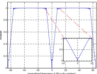
− − df f W f S P df f W f S P w I ₍₁₉₎

where the first term indicates the ICI interference within the sub-band w, the second term indicates the IBI and the third tem is the AWGN. The weighting functions versus the frequency f normalized to the sub-carrier spacing are presented in Figure 3-a and Figure 3-b respectively. These figures combined with equation (19) show the impact of the filtered CPN on the studied sub-band. Figure 3-a shows that the low frequency components (excepted DC component) of the CPN PSD have more impact on the ICI. Indeed, the small frequency components in S(f) imply a greater integration value in the first term of (19). These components are multiplied by large values of W1(f). The effect of the high frequency

components in S(f) will be cancelled by the weighting function W1(f). Figure 3-b shows that all

frequency components of the CPN PSD have an equivalent impact on the IBI. Indeed, since W2(f) is

constant in adjacent sub-bands, i.e. for n≥8, S(f) produces an equal integration value in the second term of (19). Thus, to discard the CPN effect, the engineer designers have to choose PLL filters with high cut-off frequency (cf. (4)). Moreover, a PLL having a cut-off frequency greater than the sub-carrier spacing will definitively eliminate the ICI while the IBI obstinately persists.

V. SYSTEM PERFORMANCE WITHOUT CHANNEL CODING

In this section, we will validate our theoretical model, given previously, by means of simulations. We first compare the SINR computed with (10) and (16) with the instantaneous SINR measured via Monte Carlo simulations. However, for a frequency selective slow fading physical channel and due to the channel variations of the channel caused by the mobile speed, we give the comparison between the average SINRs. The simulation assumptions in the sequel are summarized in Table 1-a.

Figure 4 illustrates the comparison between theoretical and simulated average SINRs for the BRAN A channel [27], a mean ratio Eb/N0= 20 dB and a PLL cut-off frequency of 1 MHz. The SINRs have been

measured in the first sub-band (w=0). Figure 4 shows that our theoretical model matches perfectly with simulations, even for a relatively small spreading factor (Nc=32). Moreover, it shows that the SINR

11

of MC-DS-CDMA is not straightforward from this figure. Indeed, the comparison here is achieved in terms of average SINR which could hide the advantage of a system. Moreover, the channel coding is not considered in these results. The reader could refer to [13] (section IV) for more details about the comparison of the different systems without channel coding and could refer to the next section for the systems' comparison with channel coding.

To give more insights of the CPN effect on the SINR, we define the instantaneous SINR degradation

by

[ ]

max 10 10 log SINR Deg dB SINR   = ⋅  

  where SINRmax is the SINR obtained for a perfectly synchronized system. The SINR degradation allows us to compare the sensitivity of the different spreading schemes to the CPN. Figure 5 gives the comparison between the average degradation, over channel realizations, of different spreading schemes for a BranA channel model with 18 paths [27], a mean ratio Eb/N0= 20

dB, a full load and quarter load respectively. First, we can conclude from this figure that the degradation of the different spreading schemes increases with the system load and decreases with the PLL cut off frequency. It reaches 1 dB value for a diffusion factor D ≥ 1KHz depending on the simulation assumptions. Moreover, we can conclude that the sensitivity of the 3 spreading schemes to the CPN is comparable. This conclusion could be verified as follows. The 3 spreading systems are subject to the MAI due to the loss of orthogonality between the spreading codes and the IBI due to the CPN. For a given N and a given Nc, the IBI power increases when NF decreases since the number

S=N/NF of total sub-bands increases (the number of interfering sub-bands increases as-well). However,

when NF decreases the othorgonality between codes could be conserved since the channel becomes

more flat over the considered sub-band. Then, the MAI power decreases when NF decreases. As a

consequence, for any decrease of the frequency spreading factor NF, the IBI decreases and the MAI

increases (and vice-versa). For a pure MC-CDMA system, the MAI is the dominant interference and for a pure MC-DS-CDMA, the IBI is the dominant interference. Then, the total interference power of a 2D spreading system is a trade-off between MAI and IBI.

VI. SYSTEM PERFORMANCE WITH CHANNEL CODING:APPLICATION OF THE EESM TECHNIQUE Based on the RM and FP theories, we derived in section III a simplified formula for the estimation of the instantaneous SINR at the output of the detector. However, it is desirable to evaluate the system level performance after channel decoding in terms of the BER. Therefore, an accurate relationship between the SINRs obtained at the output of the detector and the BER performance at the output of the channel decoder must be identified. Let SINR be the vector of J instantaneous SINRs received at the output of the detector. The problem of determining an accurate BER prediction method consists of finding an accurate relationship between an effective SINR value, called SINReff, computed in terms of

12

the different components of the SINR vector and the bit error probability (BEP) at the output of the channel decoder. In the literature, different solutions were proposed to evaluate the BER. In an OFDM system, [16] proposes the EESM technique which is based on the Chernoff Union bound [15] to find the effective SINR. The EESM technique expression relevant to an OFDM system yields [16][28]:

[ ] 1 0 1 ln SINR n N eff n SINR e N λ λ − − =   = − ⋅ _ _ 

∑

 (20)

where N is the number of sub-carriers, SINR[n] is the SINR obtained over the nth sub-carrier. The key point of this relation is that the parameter

λ

is unique for each pair of modulation size and channel coding rate or equivalently for each pair of MCS. It is estimated once from the link level simulations. In our study, the EESM technique must be adapted to the OFDM-CDMA systems. As shown in Figure 6, a unique SINReff is first computed for each coded set of J "2D-symbols", each composed of S QAM

symbols. It is given according to the relation:

[ ]

1 1 0 0 1 ln exp J S j eff j s SINR s SINR JS

λ

λ

− − = =    = − ⋅ _ _− __   

∑∑

 (21)

where SINRj[s] is the SINR of the sth QAM symbol transmitted on the sth sub-band of the jth 2D symbol.

J is the number of 2D symbols fed together to the channel decoder.

The BER at the output of the channel decoder is estimated from the SINReff by using a simple look-up

table (LUT). This LUT is obtained analytically or by simulations for an AWGN channel. Due to the uniqueness of the result of the relation between the BER and the SNR for each MCS, the parameter

λ

is unique for each MCS. It is independent of the channel type and of the CPN value. Thus, using the asymptotic SINR formula given by (16) with the EESM formula given by (21), we are now able to predict the BER at the output of the channel decoder without achieving system level simulations. The adaptation of the EESM technique is now to be verified by system simulations. The simulation assumptions are the same of that given in Table 1-a to which we add those of Table 1-b. The calibration procedure gives respectively

λ

=1.8 and

λ

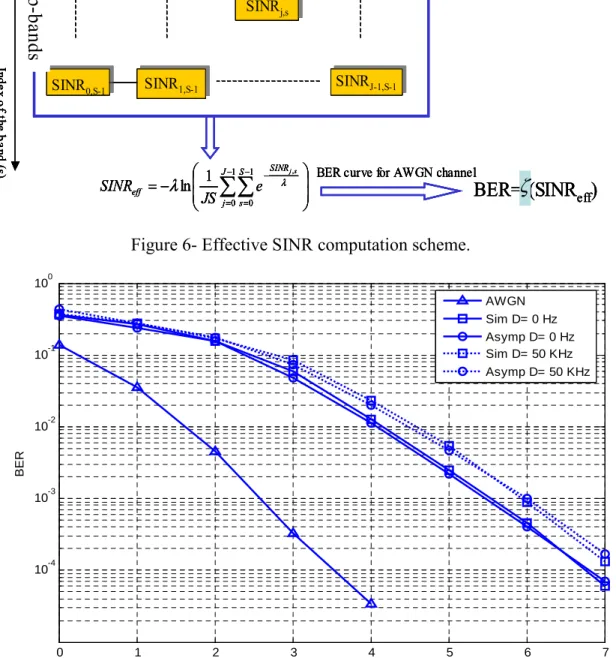
=5.5 for QPSK and 16-QAM modulations.

In figures 8 till 10, the term "Sim" in the legend stands for Monte Carlo simulation results where the term "Asymp" stands for asymptotic results using the EESM results technique. For MC-CDMA system, Figure 7 gives the comparison between both BERs obtained, first with the EESM technique using asymptotic SINR and second by simulation, in a BranA channel, a full load system and different CPN diffusion factors. In this figure, we show that the simulation results match very well the asymptotic analytical results especially for a BER<10-2. It is a double check on the EESM technique and the asymptotic evaluation. The same conclusions are verified for other OFDM-CDMA systems. Figure 7 shows that the BER at the output of the channel decoder can be accurately predicted. Also, we can conclude that the parameter

λ

is independent of the spreading system and of the diffusion factor D.

13

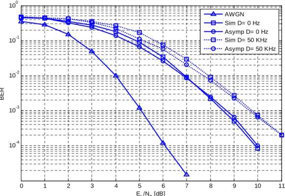
This is due to the fact that the AWGN results used as reference results do not depend on the spreading scheme. Eventually, we can conclude that at a BER=2×10-4, a loss of approximately 0.9 dB appears for a diffusion factor equal to 50 KHz. Figure 8 and Figure 9 compare between the BER obtained by simulation results and the BER obtained using the EESM technique for the OFDM-CDMA and MC-DS-CDMA systems respectively. Once again, theses figures show the accuracy of our prediction through the EESM technique with a

λ

value equal to 5.5. Again, we conclude that the parameter

λ

is independent of the spreading system and from the diffusion factor D. Also, for a BER=2×10-4, a loss of 1.5 dB and 1.1 dB are observed due a CPN having a diffusion factor D= 50 KHz. Moreover, the comparison between Figure 8 and Figure 9 shows that the OFDM-CDMA outperforms the MC-DS-CDMA due to frequency diversity obtained through frequency spreading. This diversity gain depends on the channel properties as well as on the time and frequency spreading factors.

VII. CONCLUSION

In this article, we have investigated the effect of the CPN on the performance of the 2D OFDM-CDMA spreading schemes. Based on the RM and FP theories, we have determined an analytical asymptotical expression of the SINR independent of the spreading codes. We showed the accuracy of our analysis through Monte Carlo simulations for relatively small spreading factors (Nc ≥32). Also, we presented

useful weighting functions for the RF engineers to design efficient frequency synthesizers. We showed that a PLL with high cut-off frequency is more efficient to reduce the ICI and the IBI values. We proposed an adaptation of the EESM technique to the OFDM-CDMA systems to predict the BER. Eventually, we conclude that the OFDM-CDMA systems are very sensitive to the CPN especially for large signal constellations. A loss of approximately 1 dB in terms of Eb/N0 is obtained after channel

decoding.

APPENDIX A

In this section, the 3 properties from the RM and FP theories are first defined. Then their application for the computation of (11) is detailed.

Property 1: First, we use a property initially applied in [22]. It assumes that each sequence is itself random. This assumption can be justified by the use of random scrambling codes conjointly with WH spreading sequences. Thus, if A is a (Nc×Nc), uniformly bounded, deterministic matrix and

1 ( _m(0),...., _m( _c 1)) c c c N N = − m

c where cm(l) are i.i.d. complex random variables with zero mean, unit

14 1 ( ) c N c tr N →∞ → H m m c Ac A ₍₂₂₎ m

c is obtained by the multiplication of a WH sequence with a long scrambling code. Hence, the assumptions needed for (22) are easily satisfied. This property is used to evaluate E|I0|2, E|I1|2 and

E|I2|2.

Property 2: Let C be a Haar distributed unitary matrix of size (Nc×Nu)[23]. C can be decomposed into a

vector c₀ of size Nc and a matrix U of size (Nc×Nu-1). So, C can be written as C=(c₀,U). Given these

hypothesises, it is proven in [24] that:

(

)

c N→∞ αP → − H H 0 0 UQU I c c ₍₂₃₎

α=Nu/Nc is the system load and

∑

− = − = 1 1 1 1 Nu m m u P N

P is the average power of the interfering users. The Haar

distributed assumption is only technical and will not change in the final result. The simulation results obtained in [22] with a WH spreading matrix match well the theoretical model. This lemma is used to evaluate E|I1|2.

Property 3: If C is generated from a (Nc×Nc) Haar unitary random matrix, then matrices C[s]QCH[s]

and ZH[w]HH[w,s]H[w,s]Z[w] are asymptotically free almost everywhere [26]. Based on this freeness, one can conclude:

[ ]

[ ]

(

)

(

)

(

[ ]

[ ]

)

1 1 1 [ ] [ , ] [ , ] [ ] [ ] [ , ] [ , ] [ ] c N c c c tr w w s s s w s w tr w w s w s w tr s s N →→∞ N ×N H H H H H H Z H C PC H Z Z H H Z C PC ₍₂₄₎

For definition of freeness, the reader may refer to [23] for more details.

Since we use a long scrambling code, c₀[w] and C[s] are independent for w≠s. Using (22), E|I2|2

becomes:

[ ]

[ ]

(

)

1 2 2 0 [ ] [ , ] [ , ] [ ] S s s w E I tr w w s s s w s w − = ≠ =

∑

H H H Z H C PC H Z ₍₂₅₎

Assuming that c0

[ ]

w is random, (22) is used to evaluate E|I0| 2

. Applying (23) for the computations of E|I1|2 and (24) for the computations of E|I2|2 in (25), (12) is obtained.

APPENDIX B

In this section, we derive the expectations values over the random CPN of the interferences powers.

For small angle approximation, we assume that 1 1

1 0 ] [ _<<

∑

− = N u u j q e N θ

. With this assumption, the different

15

(

)

1 1 2 2 0 0 2 ₂ 2 1 1 1 1 1 2 2 0 0 0 0 0 ( , , , , ) [ ] [ , ] ( , , , , ) [ ] ₁ [ ] 1 [ ] [ ] [ ] F T F T F T N N p q N N N N N q F q F q p q u p q q F q F w w p p q tr w w w w w p p q h wN p h wN p u N h wN p h wN p ϕ ϕ γ θ γ γ − − = = − − − − − = = = = = = +   + + =  + =   + +   + +

∑ ∑

∑ ∑

∑

∑ ∑

Z H

(

)

(

)

(

)

2 2 1 1 1 2 2 0 0 0 2 2 ₂ 1 1 1 1 2 2 0 0 0 0 ( , , , , ) ( , , , , ) [ ] [ , ] [ , ] [ ] ( , , , , ) [ ] [ ] ( ) ( ) [ ] exp 2 [ ] F F T F F T N N N p n q N N N N q F q F F q p n q u q F q w w p p q w s p n q tr w w s w s w w w p p q h wN p h sN n j w s N p n u j u if w s N N h wN p h ϕ ϕ ϕ γ θ π γ − − − = = = − − − − = = = = = = + + + − + − − ≠ + +       =

∑ ∑ ∑

∑ ∑ ∑

∑

H H Z H H Z

(

)

(

)

2 2 ₂ 1 1 1 2 2 0 0 0 2 2 ₂ 1 1 1 1 2 2 0 0 0 0 [ ] [ ] 1 [ ] [ ] [ ] [ ] [ ] exp 2 [ ] F T F F T N N N F q F q p q u q F N N N N q F q F q p n q u q F n p wN p h sN n j u N h wN p h wN p h sN n j p n u j u if w s N N h wN p θ γ θ π γ − − − = = = − − − − = = = = ≠ + + + + + + + + − − = + +           _{ }      

∑ ∑

∑

∑ ∑ ∑

∑

(26)

Using the Parseval’s identity, It can be verified that:

2 1/ 2 2 1 0 1/ 2 ( ) ( ) ( ) ( ) 1 [ ] exp 2 ( ) N F F q N u w s N p n w s N p n E u j u S f f df N θ π N θ ψ N − = − − + − − + − − = −  _{ }  _{ }      _{ }  _{ } 

∑



∫

(27)

where E[x] is the expectation value over the random variable x and

ψ

N(x) is the Dirichlet function.

By substituting (27) in (26) and applying the expectation over the CPN in (26), (12) gives way easily to (16).

For small variation approximation, we assume that the module of the CPE over one OFDM symbol is

normalised i.e. 1 1 1 0 ] [ ₌

∑

− = N u u j q e N θ

. In practice, the assumption of small variation allows the RF engineer

to have large values of CPN in such a way that its variation is small. For a MMSE equalizer, (15) yields:

[

]

[

]

[

]

[ ] [ ]

∑

∑

− = − − = + + + = + 1 0 2 1 0 2 * 1 1 N u u j N u u j F q F q F q q q e N e N p wN h p wN h p wN z θ θ _γ (28)

In simulations, we normalise the CPN values by their mean’s module during one OFDM symbol. This normalisation allows us to write (28) in a simpler form:

[

]

* 1 [ ] 2 0 [ ] ₁ [ q N j k q F q F k q F h wN p z wN p e N h wN p θ γ − − = + + = + +

∑

(29)

16

(

)

2 2 2 2 1 1 1 1 1 1 1 [ ] 2 2 2 0 0 0 0 0 0 0 [ ] [ ] ( , , , , ) 1 [ ] [ , ] ( , , , , ) [ ] [ ] F T F T F T q N N N N N N N q F j k q F p q p q k p q q F q F h wN p h wN p w w p p q tr w w w e N w w p p q h wN p h wN p θ ϕ ϕ γ γ γ − − − − − − − − = = = = = = = + + = = = + + + + +

∑ ∑

∑ ∑

∑

∑ ∑

Z H

(

)

(

)

( ) 2 2 1 1 1 2 2 0 0 0 2 1 1 1 1 [ ] [ ] 2 2 0 0 0 0 0 ( , , , , ) ( , , , , ) [ ] [ , ] [ , ] [ ] ( , , , , ) [ ] [ ] 1 ( ) ( ) exp 2 [ ] F F T F T q q N N N p n q N N N N j u k q F q F F p n q u k q F w w p p q w s p n q tr w w s w s w w w p p q h wN p h sN n w s N p n e j u N N h wN p θ θ ϕ ϕ ϕ γ π γ − − − = = = − − − − − = = = = = = + + + − + − = − + +      

∑ ∑ ∑

∑ ∑

∑∑

H H Z H H Z

(

)

[

]

1 2 1 1 1 1 1 2 2 0 0 0 0 0 [ ] [ ] 1 ( ) ( ) 1 [ ] [ ] exp 2 [ ] F F F T N N N N N N q F q F F q q p n q u k q F h wN p h sN n w s N p n j u k j u N N h wN p θ θ π γ − − − − − − = = = = = + + − + − = + − − + +      

∑

∑ ∑ ∑

∑∑

(

)

(

)

(

)

(

)

2 2 ₂ 1 1 1 1 2 2 0 0 0 0 2 2 ₂ 1 1 1 2 2 0 0 0 2 [ ] [ ] ( ) ( ) [ ] [ ] exp 2 [ ] [ ] [ ] 1 [ ] [ ] [ ] [ ] [ F F T F T N N N N q F q F F q q p n q u q F N N N q F q F q q p q u q F q F q h wN p h sN n j w s N p n u k j u if w s N N h wN p h wN p h sN n j u k N h wN p h wN p h sN θ θ π γ θ θ γ − − − − = = = = − − − = = = + + − + − − − ≠ + + + + + − + + + +       =

∑ ∑ ∑

∑

∑ ∑

∑

(

)

(

)

2 ₂ 1 1 1 1 2 2 0 0 0 0 ] [ ] [ ] exp 2 [ ] F F T N N N N F q q p n q u q F n p n j p n u k j u if w s N N h wN p θ θ π γ − − − − = = = = ≠ + − − − = + +           _{ }    _{ } 

∑ ∑ ∑

∑

(30)

Using the same computations as for the small angle approximation, (16) easily holds. REFERENCES

[1] N. Maeda, Y. Kishiyama, H. Atarashi, and M. Sawahashi, "Variable spreading factor OFCDM with two dimensional spreading that prioritizes time domain spreading for forward link broadband wireless access", Proc. IEEE Vehicular Technology Conference, vol. 1, pp. 127-132, April 2003, Jeju, Korea.

[2] A. Persson, T. Ottosson, and E. Ström, "Time-Frequency localized CDMA for downlink multi-carrier systems", IEEE 7th Int. Symp. On Spread-Spectrum Tech. & Appl., pp. 118-122, 2002, Prague, Czech Republic.

[3] T. Pollet, and M. Moeneclaey, "BER sensitivity of OFDM systems to carrier frequency offset and wiener phase noise", IEEE. Trans. Communications, vol. 43, pp. 191-193, Issue 234 Feb./March/Apr. 1995.

[4] H. Steendam, and M. Moeneclaey, "Comparison of the sensitivities of MC-CDMA and MC-DS-CDMA to carrier frequency offset", Proc. of Symp. on Communications and Vehicular Technology, pp. 166 - 173, Oct. 2000.

[5] Y. Nasser, M. des Noes, L. Ros, and G. Jourdain, "Sensitivity of OFDM-CDMA to carrier frequency offset", IEEE Int. Conf. on Communications, vol. 10, pp. 4577-4582, June 2006, Istanbul Turkey.

[6] J. Stott, "The effects of phase noise in COFDM", EBU technical Review- Summer 1998.

[7] A. Armada, "Understanding the effects of phase noise in Orthogonal Frequency Division Multiplexing OFDM", IEEE Trans. Broadcasting, vol. 47, No.2, pp. 153-159, June 2001.

[8] H. Steendam, and M. Moeneclaey, "The effect of carrier Phase jitter on MC-CDMA performance", IEEE Trans. Communications, vol. 47, No. 2, pp. 195-198, Feb. 1999.

17

[9] C. Dehos, M. des Noes, and D. Morche, "Sensitivity of MC-CDMA systems to carrier phase noise: a large system analysis", Proc. of IEEE Personnal Indoor and Mobile Radio Communications, vol. 1, pp. 407-411, Sept. 2005, Berlin Germany.

[10]Y. Nasser, M. des Noes, L. Ros, and G. Jourdain, "Sensitivity of multi-carrier two dimensional spreading systems to carrier phase noise", Proc. of IEEE Signal Processing in Advanced Wireless Communications workshop, vol. 1, pp. 1-5, July 2006, Cannes France.

[11]Y. Nasser, M. des Noes, L. Ros, and G. Jourdain, "SINR estimation of OFDM-CDMA systems with constant timing offset: a large system analysis", Proc. of IEEE Personal Indoor and Mobile Radio Communications, vol. 1, pp. 432-436, Sept. 2005, Berlin Germany.

[12]Y. Nasser, M. des Noes, L. Ros, and G. Jourdain, "The effect of clock frequency offset on OFDM-CDMA systems performance", Symp. on IEEE Communications and Vehicular Technology, vol. 1, pp. 43-47, Nov. 2005, the Netherlands.

[13]Y. Nasser, M. des Noes, L. Ros, and G. Jourdain, "Sensitivity of multi-carrier two-dimensional spreading systems to synchronisation errors”, Eurasip Journal on wireless communications and networking, vol. 2008, article ID. 561869.

[14]A. Mehrotra, "Noise analysis of phase locked loops", IEEE Trans. Circuits and systems, vol. 49, No. 9, pp. 1309-1316, Sept. 2002.

[15]Ericsson, "System level evaluation of OFDM- further considerations", TSG-RAN WG1 #35, Nov. 2003, R1-031303, Lisbon, Portugal.

[16]3GPP TSG-RAN-1, "TR 25.892: feasibility study for OFDM for UTRAN enhancement", version 1.1.0, March 2004.

[17]A. Mehrotra, "Simulation and modelling techniques for noise in radio frequency integrated circuits", PhD. Dissertation, Univ. California, Berkeley, 1999.

[18]N. Yee, JP. Linnartz, and G. Fettweis, "Multi-Carrier CDMA in indoors wireless radio networks", Proc. of IEEE Personal Indoor and Mobile Radio Communications, pp. 109-113, Yokohama Japan, 1993.

[19]A. Chouly, A. Brajal, and S. Jourdan, "Orthogonal multi carrier techniques applied to direct sequence spread spectrum CDMA systems", IEEE Globecom conf., vol. 3, pp. 1723-1728, Nov-Dec 1993, USA

[20]P. Jallon, M. des Noes, D. Ktenas, and J.-M. Brossier, "Asymptotic analysis of the multiuser MMSE receiver for the downlink of a MC-CDMA system", Proc. of IEEE Vehicular Technology Conf., vol.1, pp. 363 - 367, April 2003.

[21]D.N.C. Tse, and S.V. Hanly, "Linear multiuser receivers: effective interference, effective bandwidth and user capacity", IEEE Trans. Information Theory, vol. 45, Issue 2, pp. 641-657, March 1999.

[22]J. Evans, and D.N.C Tse, "Large system performance of linear multiuser receivers in multipath fading channels", IEEE Trans. Information Theory, vol. 46, Issue: 6, pp. 2059-2078, Sept. 2000. [23]M. Debbah, W. Hachem, P. Loubaton, and M. de Courville, “MMSE analysis of certain large

isometric random precoded systems”, IEEE Trans. Information theory, vol. 4349, Issue 5, pp. 1293-1311, May 2003.

[24]J.M. Chaufray, W. Hachem, and Ph. Loubaton, “Asymptotical analysis of optimum and sub-optimum CDMA downlink MMSE receivers”, IEEE Trans. Information Theory, vol. 50, Issue 11, pp. 2620 - 2638, Nov. 2004.

18

[25]S. Kaiser, "Multi-Carrier CDMA mobile radio systems - analysis and optimization of detection, decoding, and channel estimation", Düsseldorf: VDI-Verlag, Fortschritt-Berichte VDI, series 10, no. 531, 1998, ISBN 3-18-353110-0, pp. 48-51

[26]W. Hachem, "Simple polynomials for CDMA downlink transmissions on frequency selective channels", IEEE Trans. Information Theory, vol. 50, Issue 1, pp. 164 – 171, Jan. 2004.

[27]J. Medbo, H. Andersson, P. Schramm, and H. Asplund, "Channel models for HIPERLAN/2 in different indoor scenarios“, COST 259, TD98, Bradford, April 1998.

[28]3GPP TSG-RAN-1, "R1-030999: Considerations on the system-performance evaluation of HSDP using OFDM modulation", RAN WG1 # 34. website: www.ist-mascot.org/Members/cfm/literature/r1-031303.doc

Figure 1- OFDM-CDMA Transceiver.

Figure 2- Time Frequency grid.

S p re a d in g S sc ra m b li n g IF F T 2 D C h ip M ap p in g C P I n se rt io n ( ν ) D es c ra m b li n g E q ua li ze r F F T C ha n n el es ti m a ti o n C P R e m o v e 2 D C h ip D e m ap p in g D es p re ad in g SINR estimation Channel ] [k jq eθ C h a n ne l d e co d in g I/Q modulation I/Q modulation Channel coding Channel coding b₀[s] bNu-1[s] a₀[s] a_Nu-1[s] ] [ ˆ₀s a S o ft D e m ap p in g ] [ ˆ ₁s a_Nu− ] [ ˆ 0s b ] [ ˆ 1s bNu− S p re a d in g S sc ra m b li n g IF F T 2 D C h ip M ap p in g C P I n se rt io n ( ν ) D es c ra m b li n g E q ua li ze r F F T C ha n n el es ti m a ti o n C P R e m o v e 2 D C h ip D e m ap p in g D es p re ad in g SINR estimation Channel ] [k jq eθ C h a n ne l d e co d in g I/Q modulation I/Q modulation Channel coding Channel coding b₀[s] bNu-1[s] a₀[s] a_Nu-1[s] ] [ ˆ₀s a S o ft D e m ap p in g ] [ ˆ ₁s a_Nu− ] [ ˆ 0s b ] [ ˆ 1s bNu− F re q u en c y

N

T

N

F

N

q

s

n

T im e

19

Figure 3-a- Weighting function W1 (

f

). Figure 3-b- Weighting function W2 (

f

).

Table 1-a- Simulation parameters

FFT size (N) 64 sub-carriers

Spreading Length (Nc) 32 chips System load

α

= 1/4 and

α

= 1

Constellation QPSK

Sub-carrier spacing 312.5 KHz

Scrambling code Concatenation of 19 Gold codes of 128 chips MC-CDMA configuration NF =32, NT =1

OFDM-CDMA configuration NF =8, NT =4

MC-DS-CDMA configuration NF =1, NT =32

PLL filter with Cut-off = 100KHz b=[0.9770 -1.9541 0.9770] a=[1 -1.9881 0.9882]

PLL filter with Cut-off = 1MHz b=[0.9256 -1.8509 0.9256] a=[1 -1.8790 0.8876] Table 1-b- Additional simulation parameters

Modulation QPSK, 16-QAM Coding Rate R of Convolutional code 1/2

Polynomial code generator (133,171)o

-60 -40 -20 0 20 40 60 0 0.1 0.2 0.3 0.4 0.5 0.6 0.7 0.8 0.9 1

normalized frequency f (64 sub-carriers)

m o d u le -5 0 5 0 0.2 0.4 0.6 0.8 -60 -40 -20 0 20 40 60 0 0.2 0.4 0.6 0.8 1

normalized frequency f (64 sub-carriers)

m o d u le -10 0 10 0 0.5 1

20

Figure 4- Validation of theoretical model (BRAN A).

Figure 5- Comparison between degradations of different spreading schemes.

102 103 104 105 106 5 10 15 20 25 D [Hz] S IN R [ d B ] MC-CDMA Sim MC-CDMA Asymp OFDM-CDMA Sim OFDM-CDMA Asymp MC-DS-CDMA Sim MC-DS-CDMA Asymp 102 103 104 105 106 10-2 10-1 100 101 102 D [Hz] D E G [ d B ] MC-CDMA cut-off=106 OFDM-CDMA cut-off=106 MC-DS-CDMA cut-off=106 MC-CDMA cut-off=105 OFDM-CDMA cut-off=105 MC-DS-CDMA cut-off=105

21

Figure 6- Effective SINR computation scheme.

Figure 7- Comparison between the EESM technique with simulation EESM technique and simulation, MC-CDMA, QPSK, λ=1.8.         − =

∑∑

− = − = − 1 0 1 0 , 1 ln J j S s SINR eff s j e JS SINR λ λ

_BER=f(SINR

eff

)

BER curve for AWGN channel

SINR0,0 SINR0,0 SINR0,S-1 SINR_0,S-1 SINR1,0 SINR1,0 SINR_1,S-1 SINR1,S-1 SINRj,s SINR_j,s SINRJ-1,0 SINRJ-1,0 SINRJ-1,S-1 SINR_J-1,S-1 In d e x o f t he b a nd (s )

Index of the 2D symbol (j)

J 2D symbols

S

s

u

b

-b

a

n

d

s

        − =

∑∑

− = − = − 1 0 1 0 , 1 ln J j S s SINR eff s j e JS SINR λ λ

_BER=f(SINR

eff

)

BER curve for AWGN channel

SINR0,0 SINR0,0 SINR0,S-1 SINR_0,S-1 SINR1,0 SINR1,0 SINR_1,S-1 SINR1,S-1 SINRj,s SINR_j,s SINRJ-1,0 SINRJ-1,0 SINRJ-1,S-1 SINR_J-1,S-1 In d e x o f t he b a nd (s )

Index of the 2D symbol (j)

J 2D symbols

S

s

u

b

-b

a

n

d

s

ζ

        − =

∑∑

− = − = − 1 0 1 0 , 1 ln J j S s SINR eff s j e JS SINR λ λ

_BER=f(SINR

eff

)

BER curve for AWGN channel

SINR0,0 SINR0,0 SINR0,S-1 SINR_0,S-1 SINR1,0 SINR1,0 SINR_1,S-1 SINR1,S-1 SINRj,s SINR_j,s SINRJ-1,0 SINRJ-1,0 SINRJ-1,S-1 SINR_J-1,S-1 In d e x o f t he b a nd (s )

Index of the 2D symbol (j)

J 2D symbols

S

s

u

b

-b

a

n

d

s

        − =

∑∑

− = − = − 1 0 1 0 , 1 ln J j S s SINR eff s j e JS SINR λ λ

_BER=f(SINR

eff

)

BER curve for AWGN channel

SINR0,0 SINR0,0 SINR0,S-1 SINR_0,S-1 SINR1,0 SINR1,0 SINR_1,S-1 SINR1,S-1 SINRj,s SINR_j,s SINRJ-1,0 SINRJ-1,0 SINRJ-1,S-1 SINR_J-1,S-1 In d e x o f t he b a nd (s )

Index of the 2D symbol (j)

J 2D symbols

S

s

u

b

-b

a

n

d

s

ζ

0 1 2 3 4 5 6 7 10-4 10-3 10-2 10-1 100 E b/N0 [dB] B E R AWGN Sim D= 0 Hz Asymp D= 0 Hz Sim D= 50 KHz Asymp D= 50 KHz

22

Figure 8- Comparison between asymptotic with the EESM technique and simulation OFDM-CDMA, 16QAM, full load, Bran A channel, λ=5.5.

Figure 9- Comparison between asymptotic with EESM technique and simulation MC-DS-CDMA, 16QAM, full load, Bran A channel, λ=5.5

0 1 2 3 4 5 6 7 8 9 10 11 10-4 10-3 10-2 10-1 100 E b/N0 [dB] B E R AWGN Sim D= 0 Hz Asymp D= 0 Hz Sim D= 50 KHz Asymp D= 50 KHz 0 2 4 6 8 10 12 10-4 10-3 10-2 10-1 100 E b/N0 [dB] B E R AWGN Sim D= 0 Hz Asymp D= 0 Hz Sim D= 50 KHz Asymp D= 50 KHz