HAL Id: inria-00073473
https://hal.inria.fr/inria-00073473
Submitted on 24 May 2006HAL is a multi-disciplinary open access archive for the deposit and dissemination of sci-entific research documents, whether they are pub-lished or not. The documents may come from teaching and research institutions in France or abroad, or from public or private research centers.
L’archive ouverte pluridisciplinaire HAL, est destinée au dépôt et à la diffusion de documents scientifiques de niveau recherche, publiés ou non, émanant des établissements d’enseignement et de recherche français ou étrangers, des laboratoires publics ou privés.
Christophe Diot, François Gagnon
To cite this version:
Christophe Diot, François Gagnon. Impact of Out-of-Sequence Processing on the Performance of Data Transmission. RR-3216, INRIA. 1997. �inria-00073473�
ISSN 0249-6399
a p p o r t
d e r e c h e r c h e
Impact of Out-of-Sequence Processing on the
Perfor-mance of Data Transmission
Christophe Diot et François Gagnon
N° 3216
July 1997
PROGRAMME 1
Réseaux, systèmes, évaluation de
perfor-mances
INSTITUT NATIONAL DE RECHERCHE EN INFORMATIQUE ET EN AUTOMATIQUE
Unité de recherche INRIA Sophia Antipolis : 2004, route de Lucioles - B.P. 93 - 06902 Sophia
Antipolis cedex (France)
Transmission
Christophe Diot et François Gagnon
*Programme 1: Réseaux, systèmes, évaluation de performances
Projet RODEO
Rapport de recherche n°3216- July 1997 28 pages
Abstract: Application Level Framing (ALF) was proposed by Clark and
Tennen-house as an important concept for developing high performance applications. ALF relies in part on the ability of applications and protocols to process packets indepen-dently one from the other. Thus, performance gains one might expect from the use of ALF are clearly related to performance gains one might expect from applications that can handle and process packets received out-of-sequence, as compared to appli-catiojn that require in-order delivery (FTP, TELNET, etc.). In this paper, we exa-mine how the ability to process out-of-sequence packets impacts the efficiency of data transmission. We consider both the impact of application parameters such as the time to process a packet by the application, as well as transmission parameters such as transmission delay, loss rate and flow and congestion control characteristics. The performance measure of interest are total latency, buffer requirements, and jit-ter. We show, using experimental and simulation results, that out-of-sequence pro-cessing is beneficial only for very limited ranges of transmission delays and application processing time. We discuss the impact of this on the architecture of communication systems dedicated to distributed multimedia applications.
Key-words: ALF, Communication protocols, Out-of-sequence processing.
(Résumé : tsvp)
Version provisoire du 1997.
transmission des données
Résumé : ALF a été proposé par Clark et Tennenhouse comme un principe pour la
conception d'architectures hautes performances pour les applications distribuées multimédia. ALF s'appuie sur la capacité des applications à définir elles-mêmes les paquets (appelés ADU) qui vont ensuite être pris en charge par le système de com-munication sans aucune modification afin d'être délivrés tels-quels à l'application réceptrice. Les ADUs étant délivrées directement à l'application, ils peuvent être dès lors transmis par le réseau dans un ordre quelconque, charge à l'application récep-trice de ré-ordonner, si besoin est, les ADUs reçues avant de les délivrer. Dans ce rapport, nous étudions l'impact de la transmission hors séquence sur l'efficacité de l'application. Nous montrons que la transmission hors-séquence est fortement dépendante du temps de traitement applicatif en réception. Nous montrons aussi que dans tous les cas, transmettre et traiter les paquets hors-séquence fluidifie le trafic et réduit la gigue et les besoins en buffers.
1 Introduction
ALF was first introduced by Clark & Tennenhouse in 1990 [Clark90]. ALF questions the well-established layering model by proposing that the application and the communication stack share knowledge about the data being transmitted and processed. In particular, ALF considers that knowledge at application level about the communication stack can significantly improve the efficiency of data transmission. One consequence of ALF is that packets should be entirely designed (and specified) by the application; packets are in fact called ADUs (Application Data Units) to reflect this. ADUs are thus the units of transmission, control and
processing. This means that ADUs are transmitted to and received from the
low-level protocols atomically, and that all protocol operations are based on ADUs (i.e. no partial manipulations of ADUs are allowed and no segmentation occurs within
an ALF protocol*). Finally, ADUs are independent from each other, meaning that
they can be processed separately by the protocols and by the application. There are three important consequences to ALF based design:
• The transmission control can be tailored to the characteristics of each ADU.
Ty-pically, ADUs are classified into different types corresponding to different trans-mission protocols. It has been shown that the performance of tailored protocols can be significantly better than that of general protocols [Braun96, Zitterbart93].
• ALF makes the adaptation of applications to network conditions simpler because
of the close collaboration between the application and the transmission control protocols. This is clearly visible in the recently standardized RTP protocol [Rtp96].
• Because ADUs are independent of each other, they can be processed and
delive-red (at least in theory) by the receiving application out of sequence.
Our work focuses on this third feature of ALF. Specifically, we analyze how much can be gained with applications that can process and handle packets of-sequence. We quantify the impact of transmission parameters on the benefit of out-of sequence processing, and we provide confirmation and a detailed explanation out-of the following observations:
• Out-of-sequence processing of ADUs at a destination should significantly reduce
the total transmission delay. This is because an ADUs will not be held back by the protocol if the application can process it, and will be processed at the earliest pos-sible time. For time constrained applications, where the user can benefit from out-of-sequence information (e.g. Web browsers, image and video transmission),
mi-* Care must be taken that ADU sizes are not too large, otherwise the low-level protocol and/or parts of the network may have to segment the ADU. MTU path discovery is a mecha-nism that can be used to guarantee that ADUs will not be segmented unless routing is changed [rfc1191].
nimizing transmission delay is very important. The overall processing time (time between the start of the transmission and the end of a data delivery) can also bene-fit from out-of-sequence processing.
• The buffer requirements with out-of-sequence processing at the receiver should
always be less than or equal to the buffer requirements with ordered protocols*.
Ordered protocol re-orders ADUs before the receiving application can process it. The effect is to delay the delivery of ADUs, which results in a longer occupancy of the receiving protocol buffers.
• The application at the receiver end should suffer less jitter. With ordered
proto-cols, ADUs that are received out-of-sequence are put in a waiting list. When mis-sing ADUs finally arrive, ADUs in the waiting list are suddenly delivered to the application. This phenomenon makes the delivery of ADUs to the application burstier. The level of burstiness is affected by the percentage of out-of-sequence receptions and the processing time of each ADU (if the application processing is very long, ADUs may be received out-of-sequence, but they may be reordered be-fore the application needs them). Note that burstiness may result in bottlenecks at the receiving entity (a layer might be idle for a long time, and then receive conse-cutive bursts to process in a short time period), and in a reduced efficiency of flow control.
The confirmation of the above observations suggests that ALF is a key concept to design high performance distributed applications. However, ALF is not without cost. In particular, ALF often requires that the application and the communication stack be completely redesigned. Also, the efficiency gained by tailoring the protocol to the applications may result in non-standard solutions. Furthermore, ALF may not be simple to implement from an application point of view. For example, the definition of ADUs of appropriate sizes for applications using compression schemes may be difficult because the output of encoders is often not predictable.
The goal of this paper is to quantify the gain/cost tradeoff of ALF mentioned above. In section 2, we give an informal presentation of out-of-sequence processing. In sections 3 and 4, we analyze the impact of transmission parameters and application processing time on buffer requirements, total latency, and jitter. We use both a simulation model (described in section 3) and experiments to explore in section 4 the behavior of out-of-sequence processing for various transmission parameter settings, including transmission delay, loss rate, application processing time, flow and congestion control characteristics. We discuss in section 5 the impact of our results on the architecture of communications systems dedicated to distributed multimedia applications.
2 Issues with out-of-sequence processing
Out-of-sequence processing refers to the capability of an application to receive and process packets/ADUs in any possible order (of course, packets are normally sent "in sequence" by the sending entity). In-order delivery (or processing) refers to the delivery of ADUs to the receiving application in monotonically increasing order. The delivery order is a characteristic of the transmission; for this reason, it is a property of a protocol which is orthogonal to other transmission properties such as reliability. In this paper, we analyze reliable/out-of-sequence data transmission, and compare its performance with the classic reliable/ordered transmission such as done by TCP. That is, we study the effect of the ordering constraint on the performance of a reliable protocol.
Unreliable transmission is left for further study. When the protocol is unreliable and ordered, ADUs received out-of-sequence are delivered to the application according to application specific algorithms. This is possible because the application knows when missing ADUs should be considered lost, and how received ADUs should be delivered. An example of such an application specific delivery algorithm is the play-out buffer mechanism used in audio and video applications [Ramjee94]. This type of transmission becomes more complex to model and analyze; and it may be more the efficiency of the delivery algorithm that will be analyzed rather than the real effect of re-ordering on unreliable transmission. Furthermore, the impact of out-of-sequence processing on unreliable protocols is less significant because misordering is mostly caused by the retransmission mechanism of reliable protocols, as shown in the next section.
2.1 Why is data misordered?
Data can be misordered during the transmission due to one of the following three reasons:
• Packet retransmission in reliable protocols is the major cause of misordering.
Re-transmissions occur because of losses in the network (buffer overflow, link failu-re, etc), late acknowledgments and other types of errors. Misordering caused by retransmissions is more severe than other causes of misordering because it adds to the lost packet an additional delay of at least one round-trip-time.
• Connectionless routing is another cause of misordering. ADUs belonging to the
same application may follow different routes resulting in out-of-sequence delive-ry at the receiving entity. Route change may also be voluntadelive-ry: an application may decide to send duplicated packets on different routes in order to increase the chan-ces of succhan-cessful transmission in the face of link or node failure. Misordering due to alternate routing may result in a very small additional delay.
• Packet policing and scheduling in the network nodes can create misordering. For
packet sizes. If the sizes of ADUs differ significantly, the routers will introduce some misordering.
In today’s networks, the proportion of data received out-of-sequence depends on the network type, network load and on the type of protocol used. Let us try to quantify misordering in the Internet. It is obvious that in case of misordering caused by retransmission, the ratio of misordered packets is proportional to the loss rate, and the magnitude of misordering is proportional to the transmission delay.
Relatively little is known about misordering due to connectionless routing and packet policing/scheduling. However, preliminary measures on the Internet [Bolot96][Paxson96][Paxon97] for FTP, audio, and video traffics indicate that this type of misordering is limited to less than 1% in normal operating conditions. The magnitude of this misordering is also limited (generally to around 2 packets). Other experimental results by Handley and Ghosh (at UCL) reveal a significant level of misordering for RTP based applications. But the measured magnitude of misordering is limited to two, which is not enough to create significant perturbation on the performance at the receiving application.
On the other hand, voluntary route alternation is not relevant here as it is generally associated with unreliable transmission.
Misordering due to packet retransmission is more important, in term of frequency and magnitude. We have chosen to limit this analysis of out-of-sequence delivery to misordering introduced by retransmissions of ADUs (i.e. in case of reliable protocols). We have also decided to choose our simulation parameters for the Internet environment, where the application level loss rate can be high [Bolot93][Mukherjee94][Yajnik96].
2.2 Feasibility with respect to applications
Out-of-sequence processing is not necessarily useful, nor possible for all types of applications. Telnet and FTP for example are applications that would deliver wrong information in the case of out-of-sequence delivery. These applications could be re-written to accept a certain degree of misordering, but the code may become un-necessarily complex and the performance improvements may not be significant. Other applications such as image transmission, video server, web browser naturally accept a certain level of misordering. Raw images can be displayed totally out-of-sequence. The order in which image parts are delivered to the user is not important as long as the image is complete. JPEG and MPEG are good examples of applications that can accept to process data partially out-of-sequence. With JPEG, one can define two types of ADUs: one type of ADU to transfer the quantization and the Huffman tables, and another type of ADU to transfer the image data. Each packet of image data represents a part of the image. The JPEG specification explains that the quantization and the Huffman tables must be received in order and
before the image data. Once the tables have been received and processed, image data from the same image can be processed out-of-sequence. Raw video transmission is in the same category; within an image, packets can be processed in any order. However, images must be ordered and delivered at a defined rate. In a distributed white board application, the display of objects on the drawing board is partially ordered: objects which are not superimposed on the drawing can be displayed out-of-sequence.
In summary, we have argued that packets are often misordered by networks. When misordering is due to retransmission, the magnitude of desequencing is such that there can be a benefit in delivering packets out-of-sequence to the application. We have also shown that most distributed applications can accept a certain level of misordering in reception. In the following sections, we quantify the benefit of out-of-sequence processing of ADUs. We describe the modeling approach used in section 3, and the results of analysis in section 4.
3 The Simulation Model
Different approaches, namely analytic, simulation, and experimental approaches, are possible to tackle the problem at hand. With an analytical approach, [Harrus82] shows that re-ordering introduces additional delay in data processing. [Bacelli84] goes one step further and shows that the re-ordering delay is equal to the sum of the transmission delay, the packet processing time, and the time the packet has to wait before it can be processed by the application. He also shows that the delay a packet has to wait in order to be processed is a function of the end-to-end delay experienced by the previous packet. [Shacham91] provides numerous references on
previous analytical work on packet resequencing. He also examinesthe problem of
out-of-sequence processing and provides numerical results to illustrate the impact of out-of-sequence processing on resequencing delay and buffer occupancy. However, the mathematical complexity of the analytical models limits the possible investigations. Therefore, we decided to address the problem using simulation and experimentation. We describe the simulation model next.
3.1 The simulation model
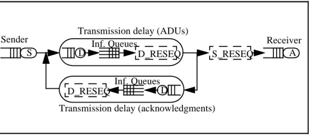
The simulation of in-order/out-of-sequence processing schemes involves the simulation of a source emitting data, the simulation of a network, the simulation of a receiver and the simulation of an end-to-end protocol to handle flow and error control (figure 1). The simulation language used is QNAP2 (Queuing Network Analysis Package, version 2) [Potier84]. The source module (S) models the emission of ADUs at a constant rate until the receiver window is full. The delay modules model the transmission delay:
• The modules with an infinite number of parallel queues (Inf. Queues) simulate the
• D is a reference server which is used for reordering purposes only.
• D_RESEQ ensures that ADUs leave the infinite queues in the same order of
se-quence they have entered these queues (or that the only misordering introduced is due to the retransmittion of ADUs).
• S_RESEQ resequences ADUs. It is used only in case of in-order transmission.
Figure 1 : Simulation Model
3.1.1 Modeling the sender
The sender has a single task, namely the emission of ADUs. To model retransmission for a reliable protocol, we use an implicit mechanism (see the section below on modeling the protocol). The emission of ADUs is rate controlled (if rate R is set to 0, the emission is bursty). The burstiness of the traffic also depends on the loss rate.
3.1.2 Modeling the receiver
The model of the receiver is simple. If an ADU can be delivered and if the receiver is idle, the receiver accepts that ADU. The receiver processes all ADUs for the same (constant) amount of time (as all ADUs approximately have the same size). While the receiver is processing an ADU, no other ADU can be delivered. The number of ADUs in the receiver buffer is limited by the maximum window size. We assume that the receiver is always able to store at least the maximum window size worth of ADUs.
3.1.3 Modeling the end-to-end control protocol
As explained in section 2, our analysis focuses on out-of-sequence processing with reliable protocols. To model reliability, we do not explicitly model an acknowledgment scheme with retransmissions. Instead, we use a mechanism where lost or corrupted data is redirected and later re-inserted in the flow emitted by the source (see Figure 1). Note that ADUs may be lost several times before reaching the
S_RESEQ
S A
Sender Transmission delay (ADUs)
Transmission delay (acknowledgments)
Receiver D_RESEQ D_RESEQ D D Inf. Queues Inf. Queues
receiver. The time before re-insertion in the emission queue is controlled by the time the receiver needs to discover the loss, and by the time an acknowledgment needs to reach the sender. We do not take into account the time it takes to process selective acknowledgments at both ends. We assume that it is constant and that it linearly affects the processing time of the receiver or the delays of the network seen by the receiver. This model is very close to what happends in a protocol like TCP.
3.1.4 Modeling the network
The network model needs to include parameters such as transmission delay, losses, and data corruption. To simplify the model, a data corruption is considered as a loss (i.e. data corruption contributes to a higher loss rate). As explained in section 2.1, misordering not caused by retransmission of ADUs is not considered in this paper.
Modeling losses
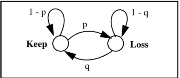
We model losses using the two state Markov chain shown in Figure 2 (often referred to as a Gilbert loss model). Losses occur while the chain is in the loss state. The average loss rate L is defined by L= p / (p+q) (where L is the loss rate).
Figure 2 : Losses with burstiness
We made various simulations with different values of p and q. We observed that the behavior of the out-of-sequence processing depends only on L, as opposed to specific values of p and q. Therefore, we chose q = 1-p without loss of generality.
Modeling transmission delays
The transmission delay in this paper is defined as the sum of the propagation delay and the buffering delays. Modeling the transmission delay is a complex task. We did not attempt to develop a general model. Instead, we have performed simulations using several specific delay distributions (hyper-exponential, exponential, constant). We have found that the performance results do not depend on the specific distribution. In this paper, the delays are modeled as the sum of a constant delay and an Erlang-3 distribution. The Erlang-3 distribution has been shown to accurately match end-to-end delays in the Internet backbone and cross country segments in the U.S.A. [Mukherjee94]. Thus, to model a delay with an average of 100 units, the simulation uses a constant delay of 50 units and an Erlang distribution with an average of 50 units and a factor k of 3, i.e. constant(50) + erlang(50,3).
p
q
1 - q 1 - p
Note that we assume that the transmission rate of the network links has a linear impact on the delay between the sender and the receiver. Also, we assume that the size of an ADU is smaller than or equal to the MTU size and therefore this size has a linear impact on the delay (no additional delay caused by fragmentation) between the sender and the receiver [Chrisment96].
3.2 Input parameters
The parameters in our simulation model are: • N: number of ADUs transmitted by the source,
•
R:
source emission rate expressed as the time interval between the emission ofconsecutive ADUs,
•
A
: acknowledgment rate (expressed in number of ADUs per acknowledgment),• W: window size (in ADUs),
•
D
: average transmission delay between the sender and the receiver,•
L
: average loss rate observed by the application, and• Ta: application processing time for one ADU at the destination.
We have examined the impact of all of these parameters (except N) over a wide range of values. The value of N is fixed to 1000. We have verified that it is sufficient to obtain a 95% confidence interval smaller than 5% of the estimated values. Each simulation has been run 5 times and the value presented in graphs below is the
average of the 5 simulation runs. We do not investigate infinite flows (i.e. N = ∞)
because the benefit on latency is not easy to quantify on infinite flows (gains are only measurable on buffer occupancy and jitter).
In the evaluation section, we analyze the effect of the transmission parameters variation on the efficiency of out-of-sequence processing. That is, we adopt a relative view where the reference points are the default values and discuss the impact of increasing or decreasing these default values for each parameter. The default values have been chosen because they correspond to realistic Internet scenarios. R, D and Ta are all interdependent. The default value is 10 for the emission rate (R), 100 for the average transmission delay (D). Ta has been chosen to be the varying parameter (on the horizontal axis). The window size (W) default value is 32, and the acknowledgment rate (A) is 2. Finally, the default loss rate (L) is 10%. Note that this is a reasonable (even though it might seem high) loss rate in the current Internet [Bolot93][Bolot96][Paxson97].
Note that D has been chosen to be able to establish a meaningful correspondence between simulation values and experimental values. For example, 10 units of time is equivalent to 10ms for Ta, D, and R.
3.3 Performance metrics
We have chosen metrics that reflect the factors of interest for time-constrained applications. Let Si be the time at which ADUi is sent. Let:
• Ri be the time at which ADUi is received by the destination entity, and
• Ai be the time at which the receiving application is ready to process ADUi
We define the following metrics.
Blocking time
Depending the relative values of Ri and Ai, two aspects of the blocking time can be considered:
• If Ai < Ri, the application blocking time Ii is the time during which the application
is waiting for the next ADU to process (Ii = max (0, Ri-Ai)). As the Ii approaches zero, the protocol is almost always able to deliver the ADUs on time and the ap-plication could not execute faster with a more efficient protocol.
• If Ai > Ri, ADU are blocked in reception waiting to be served by the application.
We define ADU blocking time Bi = max (0, Ai-Ri)). One of the goals of out-of-sequence processing is to avoid this undesirable situation.
Total time
The total time Ti is defined as the sum of application processing time, transmission time, and ADU blocking time Ti = (Si - Ri)+Bi+Ta. The total time is the most significant factor for most applications.
Gain
To give the reader a better understanding of the relative importance of performance gains, all the performance results related to the total time Ti are given in terms of the gain G. G is defined as the ratio of the total time for ordered processing minus the total time for out-of-sequence processing over the total time for ordered processing
G= (Ti(ordered) - Ti(out-of-sequence))/Ti(ordered). Thus, if G = 0.3, there is a
30% reduction of the total time when using out-of-sequence processing.
Jitter
We have chosen to define the jitter Ji as the variance of the application blocking
time Ji =
σ
2Ιi. Ji expresses the end-system jitter. We have chosen this definitionbecause the network jitter is not influenced by out-of-sequence procession of data.
Buffer occupancy
It is important to quantify buffer requirement at the receiving entity because memory is a scarce resource in some systems, and because allocating buffers is one
of the most time-consuming tasks in protocol processing. A more efficient management of the reception buffers may allow to increase the transmission rate and/or the window size. We measure the buffer occupancy in terms of the number of buffers occupied until the receiving application has finished processing all the transmitted ADUs (number of non delivered ADU at each unit of time). Note that buffers are used when the ADU blocking time is positive. This situation can happen in both in-order and out-of-sequence architectures when the transmission rate is faster than the application processing time (depending on the loss rate). This happens systematically for in-sequence processing anytime there is a loss and ADUs have to wait to be delivered in sequence.
4 Results and analysis
In this section we analyze the performance of out-of-sequence processing versus in-order processing given that the transmission is reliable and based on ALF. In the case of out-of-sequence processing, ADUs are delivered immediately to the application while in the case of in-order processing, ADUs are stored until they can be delivered in order. We first make some general observations. We then analyze the impact of the various transmission parameters on the metrics, namely the total time gain, the buffer requirements and the jitter.
4.1 General observations
We first note that the application processing time Ta clearly has a major influence on the performance improvement provided by out-of-sequence processing. When
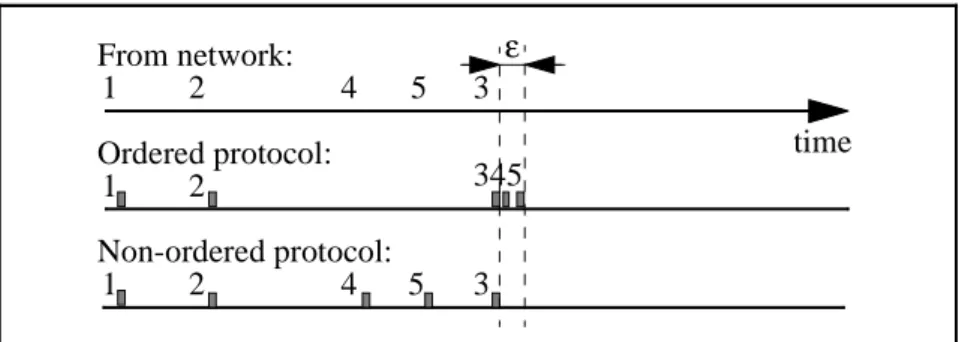
Ta tends towards 0 or ∞, out-of-sequence processing should have very little impact on Ti meaning that G tends towards 0. Figure 3 and 4 illustrate this for small and large Ta, respectively. The length of the shaded boxes represents the time to process an ADU.
Figure 3 : Small application processing times From network: Ordered protocol: Non-ordered protocol: 1 2 4 5 3 1 2 345 1 2 4 5 3 ε time
Figure 4 : Large application processing times
In figure 3, Ta is so small that processing ADUs 4 and 5 ahead of time has very little
impact (represented by ε on figure 3) on Ti. In figure 4, Ta is so large that the
protocol has enough time to recover from losses. In that case, G = 0 and there is no benefit in using out-of-sequence processing.
To examine the impact of Ta on G, it is convenient to define the operating point to be the point where the transmission rate of the sender is equal to the consumption rate of the receiver (R = Ta). If R is greater or equal to Ta, then the system is said to be stable (no buffer required in case of out-of-sequence processing, and application blocking time Ii always greater than zero). If Ta is greater than R, then the sender transmits ADUs at a rate faster than the consumption rate in reception. The system is said to be unstable as ADUs will accumulate in the reception buffers (up to infinity).
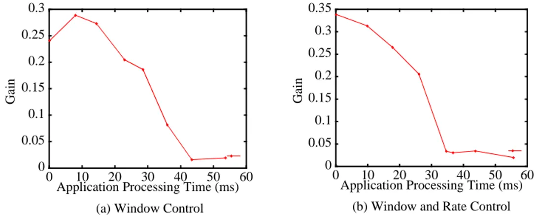
The influence of Ta on G (with default values for other parameters) has been evaluated by both experimentation (Figure 5) and simulation (Figure 6). The horizontal axis represents Ta and the vertical axis represents the gain G.
Figure 5 : Experimental results of G vs. Ta with different control schemes (A=2,
W=32, R=10 (where applicable), D=100, L=10) From network: Ordered protocol: Non-ordered protocol: 1 2 4 5 3 1 1 2 4 5 ... 2 3 4 ... time 0 0.05 0.1 0.15 0.2 0.25 0.3 0 10 20 30 40 50 60 G a in
Application Processing Time (ms)
0 0.05 0.1 0.15 0.2 0.25 0.3 0.35 0 10 20 30 40 50 60 G ai n
Application Processing Time (ms)
The experimental environment is described in the Appendix. Two different flow and congestion control scenarios have been evaluated. Figures 5 left and 6 left show the gain G for flow control based on a window mechanism. In Figures 5 right and 6 right, a rate control mechanism is added for congestion control purposes.
We analyze Figures 5 and 6 with the help of a simple model. We assume in the model that losses are isolated, and that the system has always recovered from the previous loss before the next one occurs. This could be considered as an unrealistic hypothesis, but models designed to handle cumulative loss are complex and would not bring much insight.
Let n be the number of consecutive ADUs received with no loss. We refer to this value as a "burst length" below. The value of n is directly related to the loss rate in that if n ADUs are received with no loss, the average loss rate is 1/n. Using n, we have obtained the time an ADU is blocked waiting to be served by the application, or equivalently the ADU blocking time Bi defined in the previous section. We define two functions:
• Bord is the ADU blocking time in the ordered architecture.
Bord = H (rtt + n*(Ta-R)) * (rtt + n * (Ta-R))*
• Bout is the ADU blocking time in the out-of-sequence approach. Bout = H (Ta-R) * (n * (Ta-R))
We then define the blocking time gain Gb as Gb = (Bord - Bout) / Bord.
Figure 7 represent the gain on blocking time Gb for the same conditions in the simulation and experimental settings (rtt=200, R=10) for different values of Ta and
n. The model confirms the previous results. For n=10 (or an average loss rate of
10%), Gb has the same behavior than G. However, the analytical model brings out additional interesting behavior.
We can identify 3 distinct areas in Figure 7left (these areas are better visible on Figure 7 right which shows an horizontal slice of Figure 7 left):
• Gb = 0 when Ta <= R and Ta <= R - (rtt/n). In this area, both out-of-sequence
and in-order approaches do not block ADUs. Intuitively, this is an area where, for large values of n, the ordered approach has enough time to process waiting ADUs just because of the slow transmission rate (which is slower than the application
* H(x) is the Heavyside function (also known as the step function). H(x) = 0 if x <= 0, and 1 if x > 0. Gb 1 H Ta( –R) H rtt( +n×(Ta–R)) ---– +---H rtt( H Ta+(n×–(TaR)–R))×rtt---+n×rtt(Ta–R) =
processing time). If the difference between Ta and R is large, Gb will be zero for very small values of n; i.e if R-Ta > rtt, out-of-sequence processing will not pro-vide any gain. So, it is clear that out-of-sequence processing benefits from high error rates.
Figure 6 : Simulation results of G vs. Ta with different control schemes (A=2, W=32, R=10 (where applicable), D=100, L=10)
• Gb = 1 when Ta <= R and Ta > R - (rtt/n). This is the optimal situation where
out-of-sequence processing does not block ADUs (Ta<=R), and where ordered transmission blocks ADUs. That is where the gain on the total time G will be the highest. An important result is that whatever the relative values of the transmis-sion parameters, the maximum gain area will always exist because Ta=R is the asymptot for the Ta=R-(rtt/n) function. But the surface of the maximum gain area tends to zero for small round-trip-times or large transmission rates, whatever the application processing time and the loss rate are.
• Gb is decreasing exponentially to zero when Ta > R (in that case, Gb= rtt / (rtt+n*(Ta-R))). The decreasing speed is directly proportional to n and Ta-R (the
influence of the rtt is negligible as it appears on both sides of the function). So, the higher the gain is, and the bigger the difference between Ta and R is, the faster the gain of out-of-sequence processing is reaching zero.
Analysis and results above yeld the following observations:
The model confirms simulation and experimental results
The first important observation is that G is never negative, i.e. in the worst case, out-of-sequence processing is never less efficient than ordered processing. Simulation and experimental results show similar behaviors that are confirmed by the model. Note that the behavior of G on figure 5 left for small values of Ta (which is different from that of Figure 6 left, and 7 left) can be simply explained by slight variation in the experimental conditions that make that the phenomenon observed for n > 15 on figure 7 left appeared earlier (i.e. for n=10) in experimental conditions.
0 0.05 0.1 0.15 0.2 0.25 0.3 G ai n
Application Processing Time (ms) 0 0.05 0.1 0.15 0.2 0.25 0.3 0.35 G a in
Application Processing Time (ms)
(a) Window Control (b) Window and Rate Control
16 Christophe Diot et François Gagnon
Figures 5 and 6 also show that the gain is higher with rate control than without (or with R=0). The model shows that when R = 0, then R < Ta and Gb (which is the maximum gain that can be obtained on total time) decreases exponentialy with Ta. Intuitively, the effect of rate control is to space ADUs so that they do not accumulate in reception. This explains that ADUs wait less with rate control, and in both in-order and out-of-sequence cases.
Figure 7 : Gb vs. Ta and n, for rtt = 200ms and R = 10ms (analytical results)
The maximum gain is limited to about 30%
The maximum gain observed in figures 5 and 6 is around 30%. The analysis of the blocking time gain Gb does not help us to evaluate the maximum gain G. But an intuitive analysis shows that the transmission parameters that have the highest influence on G are the loss rate (the higher the loss, and the more delay received packets will have to wait), and the round-trip-time (a large round trip delay delays the reception of the lost ADUs, and consequently the delivering of blocked ADUs). The impact of these two parameters will be analyzed in the following section. However, the analytic study shows that for high loss rates (e.g, for small values of
n) or large round-trip-times the application processing time range that provides a
maximum gain is larger than with small loss rates and small round trip times.
Out-of-sequence processing is not very useful for large application processing times.
The gain on total time can be important for small values of Ta. It turns out that the constraint imposed by the receiver window on the emission of ADUs causes a cumulative effect (the intuitive discussion did not consider any flow or congestion control). If an ADU is lost, the receiver buffers may be filled with out-of-sequence ADUs. In this case, the sender is not allowed to send until the lost ADU(s) is/are recovered. Also, because the processing time is small, the receiver stays idle and the protocol is never able to recover the lost time. This is confirmed by the analytical model which shows that for lower loss rates (or for larger windows as the window
2 4 6 8 10 12 14 16 18 20 10 20 30 40 50 60 70 80 90 100 Ta Burst costord (x) R gain (x,y) 0 5 10 15 20 25 30 35 40 45 50 0 5 10 15 2025 30 3540 0 0.5 1 Ta Burst Gain Burst Ta Gb Gb = 1 Gb = 0 Gb decreases to 0 R Burst Ta
limits the number of ADUs that can be accumulated in reception), the ordered protocol has enough time to process blocked ADUs and the two approaches become equivalent. On the other hand, when Ta is sufficiently large, the two control scenarios provide the same results because the protocol has sufficient time to recover lost ADUs before they are needed by the application. The point when out-of-sequence processing becomes useless corresponds, for the current transmission parameters setting, to be approximately 40ms. This number is confirmed by the analytical model.
As shown with the analytical model, the application processing time range in which out-of-sequence processing is efficient is determined by the relative values of the transmission delay (D) and the transmission rate (R). These parameters will be analyzed in detail later in this section. At this stage of the discussion, we make two observations:
• Maximum efficiency is reached when the application processing time Ta is
smal-ler than or equal to the emission rate R and when n is small, e.g for significant loss rates.
• Out-of-sequence processing is beneficial when application processing time is
small in comparison to the transmission delay.
Typical values for transmission delay in a normally loaded Internet are in the 50ms-300ms range. Application processing time of course depends on specific applications. On a Sparc 20, processing an audio packet takes approximately 0.2ms with ADPCM coding and close to 4ms with GSM coding; processing a video packet takes at least (related to its size and encoding scheme) 50ms. Hence, out-of-sequence processing in the audio application would be beneficial. But audio is a continuous media application and we explained earlier that the total time reduction for this type of application is not sensitive. For the video application, out-of-sequence processing would be useful for transmision delays that would be 10 times the application processing time. Consequently, from a total time point of view, the interest of out-of-sequence processing is limited to application such as web browsers or video or image transmission with low processing requirements on the receiving side.
4.2 Impact of the transmission parameters on G
In the following section, we analyze the impact of the transmission parameters (defined in section 3.2) on the gain G. All results have been obtained by simulation, and simple models used to explain a specific behavior.
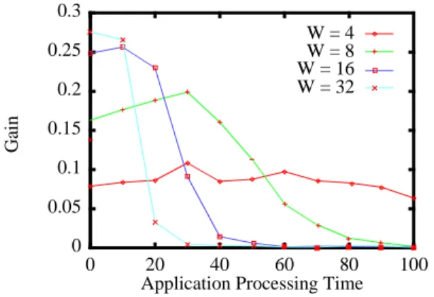
4.2.1 Gain vs. window size
Figure 8 shows the influence of the window size W on G. Increasing W has two effects on G:
• it increases the maximum gain, and
• it reduces the range of application processing time where G is maximum.
Misordering being due to losses, an ordered processing scheme based on window flow control will block the receiving application until retransmitted ADUs are received. On the other hand, the out-of-sequence processing scheme allows the receiving entity to process any ADU in the window while waiting for the missing ADUs (protocols have more time to recover loss while the application is processing ADUs).
Figure 8 : G vs. Ta with different window size (A=2, R=10, D=100, L=10)
This is easy to explain with our model. The effect of the window on the ADU blocking time is to put a maximum limit on the number of ADUs that can be accumulated in the receiver buffers. If this number is larger than the probability of having a loss occuring in the window, then the window mechanisms has no effect on the blocking time and G is the one that would be obtained without window control. If the window is small, then the window control mechanism limits blocking time in both situations. This is equivalent to have a small value of n.
Note that in Figure 8, the maximum gain is obtained for window sizes larger than 16. Consider 10% loss rate in our simple model, meaning n approximately equal to 10. For window sizes larger than 10, the gain should be 1. The difference between
W=16 and W=32 can be explained as follows: if the first ADU of the window is lost,
then the retransmitted ADU will reach the receiver after one round-trip-time, or 200ms later. Once this ADU is received, the blocking time start decreasing. The 200ms delay gives enough time to accumulate 20 ADUs in the windows. With a window size of 32 ADUs, the flow control mechanism does not block before the retransmitted ADU reaches the receiver, and the window mechanism has no impact. With a window size of 16, the window will stop the number of accumulated ADUs before the retransmited ADU is received. Consequently, the number of ADUs to process upon reception of the retransmission will be smaller, and the difference with out-of-sequence processing will be less important.Consequently, the maximum gain
0 0.05 0.1 0.15 0.2 0.25 0.3 0 20 40 60 80 100 G ai n
Application Processing Time W = 4 W = 8 W = 16 W = 32
area can be increased by choosing a window size which depends on the end-to-end delay.
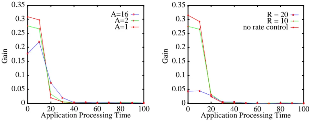
4.2.2 Gain vs. acknowledgment strategy
The acknowledgment strategy is based on selective acknowledgments. Each time n ADUs are received, an acknowledgment is returned with the sequence numbers of the received ADUs. More frequent acknowledgments should benefit both delivery schemes; less frequent acknowledgments, by contrast, seem to degrade the performance in the presence of the out-of-sequence processing scheme as shown in Figure 9 left. Less frequent acknowledgments dampen the "cumulative effect" of the receiver window because the sender cannot fill the window as soon as it could. Very low acknowledgment frequencies will block both processing schemes.
A cumulative acknowledgment strategy would have given even less gain to out-of-sequence processing. A positive acknowledgment for packet n is sent when all packets until sequence number n have been previously and correctly received. Cumulative acknowledgments act as synchronization points for both schemes.
Figure 9 : G vs. Ta with different acknowledgment frequency (Left; W=32, R=10,
D=100, L=10) and to the transmission rate (right, A=2, W=32, D=100, L=10) 4.2.3 Gain vs. transmission rate
Figure 9 right confirms that the addition of rate control reduces the benefit of out-of-sequence processing. As already explained, spacing packets increases the inefficiency of the application receiving entity, which spends more time to wait for ADUs. For example, with a transmission rate of 20 ms and an application processing time of 10 ms, the receiver is idle approximately 50% of the time. Note that it is difficult in practice to choose the rate, window size, and acknowledgment frequency so as to optimize the efficiency of out-of-sequence processing. This is because these parameters are usually chosen (dynamically) to provide efficient flow and congestion control on data transmission.
0 0.05 0.1 0.15 0.2 0.25 0.3 0.35 0 20 40 60 80 100 G ai n
Application Processing Time A=1 A=2 A=16 0 0.05 0.1 0.15 0.2 0.25 0.3 0.35 0 20 40 60 80 100 G ai n
Application Processing Time no rate controlR = 10
4.2.4 Gain vs. transmission delay
We have shown that the benefits of out-of-sequence processing increase with transmission delays D. Figure 10 left shows that increasing the delay affects primarily the range of application processing times in which out-of-sequence processing is efficient, but not the gain itself. This is confirmed by the analysis which shows that the longer the round-trip-time, the larger the range of the maximum gain area.
This range increases with increasing delays. For D=500ms, out-of-sequence processing efficiency remains stable for application processing times up to 50ms. With 10% loss then it takes one second for an ADU to be retransmitted. This means that if the first packet of the window of 10 ADUs is lost, the application will only wait for it 500 - 9*50 = 50ms (during the 500ms, it will process -in both delivery schemes- the ADUs from the previous window). For Ta=100ms, both delivery schemes become equivalent because retransmitted ADUs arrive when the application finishes to process the previous window. So, G increases with D. Out-of-sequence processing does not provide significant performance gains for short transmission delay environments (D small with respect to Ta) because lost ADUs can be recovered very quickly.
Figure 10 : G vs. D (left), and D/Ta (right) (A=2, W=32, R=10, L=10)
Figures 10 right shows an important result, namely that the ratio D/Ta is constant. In other words, the efficiency of out-of-sequence processing is constant for any couple (D, Ta) provided the ratio D/Ta is constant. If D/Ta < 5, or if D is less than 5 times
Ta, out-of-sequence delivery is useless. The gain will be maximum for D/Ta > 10,
or transmission delays greater than 10 times the application processing time. We explain this property using the analytical model. The gain on the blocking time Gb
has been evaluated for Ta larger than or equal to R*. The analytical result is not
* For R>Ta, Gb = 0 or 1. The behavior of G in this area has already been studied early in this section. 0 0.05 0.1 0.15 0.2 0.25 0.3 0.35 0 20 40 60 80 100 G ai n Ta D = 10 D = 100 D = 500 0 0.05 0.1 0.15 0.2 0.25 0.3 0.35 0 5 10 15 20 G ai n D/Ta Ta=20 Ta=10 Ta=50
Impact of Out-of-Sequence Processing on the Performance of Data Transmission 21
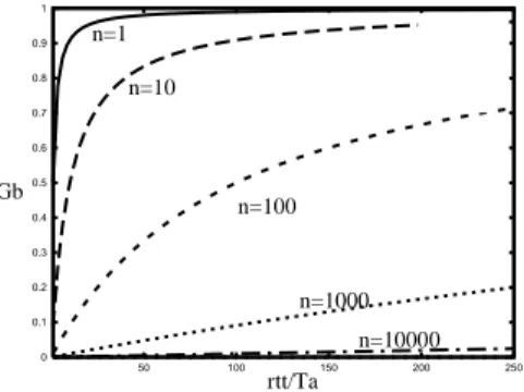
exactly similar to the simulation result, but they both are constant in regard to Ta. Moreover, the equation of Gb (given section 4.1) reveals that it is also constant whatever the value of R is. Consequently, Figure 11 shows that when Ta>R, the gain is significant only if rtt/Ta is greater than approximately 20, and that this gain depends only on the loss rate (expressed by n in Figure 11).
Figure 11 : G vs. rtt/Ta, for any value of R and Ta (analytical results)
Typical values for the average transmission delay in the current Internet are 10ms over LANs, 50 to 10ms nationwide, and 200 to 300ms across continents. These values mean that the range of application processing times for which out-of-sequence processing is useful, is small. In the case of local transmission, Ta should be less than 1ms; nationwide, less than 10ms; and cross continent less than 50ms. Thus, multimedia applications incur little benefit in using out-of-sequence processing in local and nationwide transmissions. However, transcontinental transmission would result in important gains.
4.2.5 Gain vs. packet losses
Figure 12 shows the impact of application level ADU loss on G. Losses have a dramatic effect on the performance of the in-order delivery scheme. When the loss rate is high, the sender of in-order delivery blocks much more frequently because of the receiver window becoming full (more often waiting for one or more rtt before any new ADU can be transmitted). Figure 12 left shows the efficiency of out-of-sequence processing with varying loss rates for different values of Ta. It shows that the maximum expected benefit is around 90% for unrealisticly high loss rates (60%). The value of G shows similar results to those obtained analytically (figure 7 left). It can be seen on both figures that the maximum gain is reached for Ta < R. Note that we have chosen loss rates that go all the way up to 40% because such loss rates, even though very high, are not uncommon at all in the current Internet (refer to the many recent measurement studies in [Yajnik96], [Mukherjee94][Bolot93] that support this).
0 0.1 0.2 0.3 0.4 0.5 0.6 0.7 0.8 0.9 1 50 100 150 200 250 Gain rtt/Ta gn (x,1) gn (x,10) gn (x,100) gn (x,1000) gn (x,10000) Gb n=1 n=10 n=100 n=1000 n=10000 rtt/Ta
Figure 12 : G vs. Ta for different packet loss (A=2, W=32, R=10, D=100)
4.3 Buffer requirements
The results on buffer requirements and jitter shown in this and the next section are experimental (the implementation environment is described in the Appendix). We have not gathered the equivalent results using simulation because these results can be explained without ambiguity. Figure 13 shows the receiver buffer size used while transmitting 100 ADUs for in-order (Figure 13 left) and out-of-sequence (Figure 13 right) processing schemes. Clearly, the average buffer occupancy and the variance on buffer occupancy is much less for out-of-sequence processing. Note that the buffer size often increases by more than one ADU because our algorithm gives precedence to incoming ADUs from the network over the processing of ADUs. For a window size of 32 ADUs (with one buffer per ADU), the maximum buffer size used with ordered delivery does not exceed 28. With out-of-sequence delivery, the size never exceeds 10.
Figure 13 : Buffer requirements (experimental results with W=32, R= 10, L= 10, D= 100, A=4)
It is important to notice too that the traffic at the receiving application is smoother with out-of-sequence processing than with in-ordered (it can be expressed by the variance on the buffer occupancy). The window effect is more visible on Figure 13
0 0.1 0.2 0.3 0.4 0.5 0.6 0 20 40 60 80 100 G a in
Application Processing Time L=0 L=5 L=10 L=20 L=40 L=60 0.4 0.5 0.6 0.7 0.8 0.9 1 0 10 20 30 40 50 60 G ai n Loss Rate (%) Ta=00 Ta=10 Ta=15 Ta=20 Ta=30 in-order out-of-sequence 0 5 10 15 20 25 30 0 500 1000 1500 2000 B u ff er S iz e (A D U s) Time (ms) 0 5 10 15 20 25 30 0 500 1000 1500 2000 B u ff e r S iz e (A D U s) Time (ms)
left, where three buffer occupancy peaks are visible. The amplitude of the peaks, as well as the peaks themselves, are more difficult to see when out-of-sequence delivery is used (Figure 13 right).
Figure 13 also confirms that the total latency is reduced with out-of-sequence processing: while an ordered approach needs close to 2500ms to deliver 100 ADUs, the out-of-sequence approach needs less than 1500ms (that gives G=40%)
4.4 Blocking time and jitter
Figures 14 left and 14 right show the (experimental) distribution of application blocking times for the ordered delivery of 100 ADUs.
Figure 14 : Application blocking time (experimental; W=32, N=100, R=10, L=10,
D=100, A=8)
With ordered delivery, the blocking times are longer. This is because at the beginning of the transfer, the receiver is waiting for missing ADUs while ADUs with larger sequence numbers fill the buffers. With out-of-sequence processing, the receiver does not wait much because it processes other ADUs while missing ADUs are recovered. Consequently, jitter (which we defined as the variance of the blocking time) is significantly less for out-of-sequence delivery (more than 30%).
5 Conclusions
We have analyzed the efficiency of out-of-sequence processing for reliable protocols. We have chosen reliable protocols because misordering is mostly due to retransmission in networks such as the Internet (see section 2).
The impact of out-of-sequence processing is spectular on receiver buffer occupancy (around 70% gain) and jitter (approximately 30% gain). For buffer occupancy and jitter, the gain can be observed with all types of applications. A positive side effect of out-of-sequence processing is also to smooth the traffic as it passes to the application. The gain on the total transmission time (Ti) is limited by the application nature and the networking conditions. It is correlated to all the transmission
in-order out-of-sequence 0 50 100 150 200 250 300 350 400 450 500 0 500 1000 1500 2000 B lo ck in g T im e (m s) Time (ms) 0 50 100 150 200 250 300 350 400 450 500 0 500 1000 1500 2000 B lo ck in g T im e (m s) Time (ms)
parameters (window size, transmission rate, and acknowledgment frequency), but the one that have the largest impact on the total time are loss, transmission delay, and application processing time:
• A high loss rate can increase the gain up to 50% for 60% ADUs loss rate.
Howe-ver, such loss rates are unrealistically high. For "average" loss rates, the gain on total transmission time is limited to 30%.
• Benefit on total time is limited to a very narrow range of application processing
times. Only increasing the transmission delay can extend this application proces-sing time range.
• Together with the two previous results, the application processing time should be
less than the emission rate to maximize the benefit. If R is smaller than Ta (e.g. the emission rate is faster than the consumption rate), then window control is compulsory to guarantee the stability of the system and the benefit of out-of-se-quence processing is almost null.
• The highest profit are reached for a transmission delay that is at least 10 times the
application processing time.
There are important consequences of this work on the architecture of multimedia applications and communication systems:
• Multimedia applications (characterized by non negligible processing times) will
benefit from out-of-sequence processing for communications characterized by long transmission delays. The profit for local communication being limited to very short application processing times. This means that multimedia applications should be designed with cheap decoding costs. Note that this corresponds to the current state of the art, where decoding is cheaper than ancoding (examples: H261, MPEG, etc.)
• Within the framework of ALF, out-of-sequence delivery is a prerequisite to larger
improvements. It reduces delays, buffer occupancy, and jitter. It also allows for more control at the application level and makes it easier to provide QoS guaran-ties. In the case of reliable multicast applications, out-of-sequence processing maintains low latency and reduces delays among all group members (each group member can receive in a different order as the application knows how to deliver information).
• Out-of-sequence processing is very profitable on the total time for the
transmis-sion of short size data flows, with siginificant loss rates, and long end-to-end network delays. This makes Web browsers perfect candidates for such a delivery scheme. In particular, HTTP could be modified to allow the Web traffic to be pro-cessed out-of-sequence.
Out-of-sequence delivery could also benefit from other types of misordering. Today, on the Internet, misordering due to alternate routing or to routers scheduling
is limited. The advent of operator based addressing and of service guaranty could change this situation. Anyhow, misordering due to routing and scheduling has a limited magnitude, that will result in minimal benefits (when misordering is due to loss, the magnitude of misordering is proportional to the round-trip-time).
Acknowledgments
Jean Bolot helped as well in the model design and in the paper improvement. Also thanks to Jon Crowcroft (UCL), Christian Huitema (BELLCORE), Aruna Seneviratne (UTS), Don Towsley (U. Mass.), and Mostafa Ammar (Georgia Tech.) for reviewing early versions of this paper and valuable comments.
References
[Baccelli84] F. Baccelli, E. Gelembe, and B. Plateau. "An End-to-End Approach to the Resequencing Problem". Journal of the ACM. Vol. 31, No. 3, Pp. 474-485. July 1984.
[Bolot93] J-C. Bolot. "End-to-end packet delay and loss behavior in the Internet". Proceedings of ACM SIGCOMM ' 93, San Fransisco, CA, September 1993. [Bolot96] informal discussion with Bolot, Paxon, and Keshav. Spring 1996. [Braun96] T. Braun, I. Chrisment, C. Diot, F. Gagnon, L. Gautier, "ALFred, a Protocol Compiler for the Automated Implementation of Distributed Applications' ' , to be published in the proceedings of HPDC-5 symposium. IEEE press. Syracuse. August 6-9 1996.
[Chrisment94] I. Chrisment, "Impact of ALF on Communication Subsystems Design and Performance", Proceedings of the First International Workshop on High Performance Protocol Architectures 94, Sophia Antipolis, December 1994.
[Chrisment96] I. Chrisment and C. Huitema, "Evaluating the Impact of ALF on Communication Subsystems Design and Performance", to be published in Journal For High Speed Networks in 1996.
[Clark90] D. D. Clark and D. L. Tennehouse, "Architectural Considerations for a New Generation of Protocols", Proceedings of ACM SIGCOMM, 1990.
[Diot95] C. Diot, C. Huitema, T. Turletti, "Multimedia Application should be Adaptive' ' , HPCS Workshop. Mystic (CN), August 23-25, 1995.
[Harrus82] G. Harrus et B. Plateau. "Queing Analysis of a Reordering Issue. IEEE Transactions on Software Engineering. Vol. SE-8, No. 12, Pp. 113-122. March 1982.
[Yajnik96] M. Yajnik, J. Kurose, D. Towsley, "Packet Loss Correlation in the MBone Multicast Network". IEEE Global Internet Conference. London, November 1996.
[Mukherjee94] A. Mukherjee, "On the Dynamics and Significance of Low Frequency Components of Internet Load", Internetworking Research and Experience, Volume 5, Number 4, Dec. 1994.
[Paxson96] V. Paxon. "End-to-End routing Behavior in the Internet". Proceedings of ACM SIGCOMM ’96. Pp. 25-38. Stanford (CA). August 1996.
[Paxson97] V. Paxson. "End-to-end Internet Packet dynamics". Proceedings of ACM SIGCOMM ’97. Cannes. September 1997.
[Potier84] D. Potier, "New Users’ Introduction to QNAP2", Technical Report no. 40, INRIA, 1984.
[Rfc1191] J. Mogul, S. Deering. Path MTU Discovery. IETF RFC 1191. November 1990.
[Rtp96] H. Schulzrinne, S. Casner, R. Frederick, V. Jacobson, "RTP: A transport protocol for real-time applications' ' , RFC 1889, January 1996.
[Ramjee94] R. Ramjee, J. Kurose, D. Towsley, H. Schulzrinne, "Adaptive playout mechanisms for packetized audio applications in wide-area networks' ' , Proceedings of Infocom ' 94, Toronto, Canada, pp. 680-688, April 1994.
[Shacham91] N. Schacham and D. Towsley. "Resequencing Delay and Buffer Occupancy in Selective Repeat ARQ with Multiple Receivers". IEEE Transactions on Communications. Vol. 39, No. 6, Pp. 928-937, June 1991.
[Zitterbart 93] M. Zitterbart, B. Stiller et A. Tantawy. "A model for flexible high performance communication subsystems", Journal on Selected Areas in Communications, May 1993.
Appendix: The experimental environment
Figure 15 shows the experimental environment composed of a sender and a receiver communicating through a local area Ethernet. The task of the source is to emit N ADUs as fast as possible. The protocol delivers ADUs to a module that simulates losses in the network and then to a module that simulates delay. Finally, ADUs are sent through the network using UDP.
The experiments presented in this paper were not performed on the wide area Internet because we wanted to control and vary delays and losses. However, we have performed some experiments on the Internet to confirm that results based on similar loss and delay distributions are consistent.
Because we experiment on a local network, we had to control manually the loss rate and the delay. The models used for these two processes are those developed for the simulation environment.
Figure 15 : Experimental Model
At the receiving entity, the protocol fetches ADUs from UDP buffers and delivers them to the application as soon as possible. The application processes ADUs for a fixed amount of time (this assumption is realistic in the ALF framework, and it has no effect on the evaluation results). The application stays idle when there are no ADUs to be processed and never keeps the CPU for a long period of time. Also, the control protocol is given priority over the application.
We use both static window control for end-to-end flow control and rate control for congestion control. The window is sized by the receiving entity and is a function of the number of buffers that it has available for reception. The flow control window size is fixed (it is realistic because it is only dedicated to end-to-end control). For simplicity, the ADU emission rate stays constant and ADUs are emitted (one by one) at this rate. Other rate control schemes could be implemented, but we have chosen this one because it preserves the smoothness and the continuity of the traffic. The acknowledgment mechanism is based on selective positive acknowledgments. In the context of ALF, selective acknowledgment is more appropriate than schemes such as go-back-n because it gives finer control over retransmissions. The receiver sends a selective acknowledgment after the reception of n ADUs, where n is smaller than the window size. Retransmission of ADUs has been evaluated with and without rate control. In the absence of rate control, ADUs are retransmitted as soon as a loss is detected; otherwise, the ADU can be delayed by the rate control mechanism. Both retransmission strategies exhibit similar behavior.
The experiments were performed between an ULTRA Sparc 1 and a Sparc 20, both running Solaris 2.5. Both workstations, as well as the network, were lightly loaded. Note that we assume that the network is relatively stable. Hence, the loss rate, the average transmission delay, and the variance of delay are also constant.
To avoid bottlenecks that would affect the results in the experimental environment (i.e. speed and available bandwidth of the network, and the capacity of the UDP buffers), we used a moderate window size (maximum 64), a moderate emission rate (every 10ms) and a moderate ADU size (512 bytes, well below MTU size). We have also adjusted the UDP buffer size so that ADUs at the receiver are never discarded because of UDP-level blocking.
Source Delay Ethernet Receiver Loss Sender Protocol Network