Investigation of subauroral ion drifts and related field-aligned currents and ionospheric Pedersen conductivity distribution

HAL Id: hal-00317271

https://hal.archives-ouvertes.fr/hal-00317271

Submitted on 19 Mar 2004

HAL is a multi-disciplinary open access

archive for the deposit and dissemination of

sci-entific research documents, whether they are

pub-lished or not. The documents may come from

teaching and research institutions in France or

abroad, or from public or private research centers.

L’archive ouverte pluridisciplinaire HAL, est

destinée au dépôt et à la diffusion de documents

scientifiques de niveau recherche, publiés ou non,

émanant des établissements d’enseignement et de

recherche français ou étrangers, des laboratoires

publics ou privés.

field-aligned currents and ionospheric Pedersen

conductivity distribution

S. Figueiredo, T. Karlsson, G. T. Marklund

To cite this version:

S. Figueiredo, T. Karlsson, G. T. Marklund. Investigation of subauroral ion drifts and related

field-aligned currents and ionospheric Pedersen conductivity distribution. Annales Geophysicae, European

Geosciences Union, 2004, 22 (3), pp.923-934. �hal-00317271�

SRef-ID: 1432-0576/ag/2004-22-923 © European Geosciences Union 2004

Annales

Geophysicae

Investigation of subauroral ion drifts and related field-aligned

currents and ionospheric Pedersen conductivity distribution

Alfv´en Laboratory, Royal Institute of Technology, Stockholm, Sweden

Received: 4 December 2002 – Revised: 10 September 2003 – Accepted: 8 October 2003 – Published: 19 March 2004

Abstract. Based on Astrid-2 satellite data, results are

pre-sented from a statistical study on subauroral ion drift (SAID) occurrence. SAID is a subauroral phenomenon characterized by a westward ionospheric ion drift with velocity greater than 1000 m/s, or equivalently, by a poleward-directed electric field with intensity greater than 30 mV/m. SAID events occur predominantly in the premidnight sector, with a maximum probability located within the 20:00 to 23:00 MLT sector, where the most rapid SAID events are also found. They are substorm related, and show first an increase in intensity and a decrease in latitudinal width during the expansion phase, followed by a weakening and widening of the SAID struc-tures during the recovery phase. The potential drop across a SAID structure is seen to remain roughly constant during the recovery phase.

The field-aligned current density and the height-integrated Pedersen conductivity distribution associated with the SAID events were calculated. The results reveal that the strongest SAID electric field peaks are associated with the lowest Ped-ersen conductivity minimum values. Clear modifications are seen in the ionospheric Pedersen conductivity distribution as-sociated with the SAID structure as time evolves: the SAID peak is located on the poleward side of the corresponding region of reduced Pedersen conductivity; the shape of the re-gions of reduced conductivity is asymmetric, with a steeper poleward edge and a more rounded equatorward edge; the SAID structure becomes less intense and widens with evolu-tion of the substorm recovery phase. From the analysis of the SAID occurrence relative to the mid-latitude trough position, SAID peaks are seen to occur relatively close to the corre-sponding mid-latitude trough minimum. Both these features show a similar response to magnetospheric disturbances, but on different time scales - with increasing magnetic activity, the SAID structure shows a faster movement towards lower latitudes than that of the mid-latitude trough.

From the combined analysis of these results, we conclude that the SAID generation mechanism cannot be regarded

ei-Correspondence to: S. Figueiredo

(sonia.figueiredo@alfvenlab.kth.se)

ther as a pure voltage generator or as a pure current genera-tor, applied to the ionosphere. While the anti-correlation be-tween the width and the peak intensity of the SAID structures with substorm evolution indicates a magnetospheric source acting as a constant voltage generator, the ionospheric mod-ifications and, in particular the reduction in the conductivity for intense SAID structures, are indicative of a constant cur-rent system closing through the ionosphere. The ionospheric feedback mechanisms are seen to be of major importance for sustaining and regulating the SAID structures.

Key words. Ionosphere (mid-latitude ionosphere; electric

fields and currents; ionosphere-magnetosphere interactions)

1 Introduction

Strong poleward electric fields associated with intense west-ward ionospheric plasma flow are a relatively common fea-ture observed at subauroral latitudes in the evening to pre-midnight local time sector during substorm activity. Denoted as subauroral ion drifts (SAID) or equivalently, as subauroral electric fields (SAEF), this phenomenon has been the subject of many studies reported by several authors during the last three decades. Although different measurement techniques and different definitions were used, there are several features of this phenomenon generally agreed upon. The SAID phe-nomenon is a manifestation of magnetosphere-ionosphere coupling outside of the auroral region, characterized by west-ward ion drifts with velocities greater than 1000 m/s by many of the authors (Anderson et al., 1991; Galperin et al., 1997; Burke et al., 2000). Some authors have focused on the corre-sponding intense poleward-directed electric fields, reporting events with intensities greater than approximately 30 mV/m (Smiddy et al., 1977; Maynard, 1978; Maynard et al., 1980; Rich et al., 1980; Karlsson et al., 1998). SAID structures are confined to latitudinally narrow regions (0.1◦–2◦ CGLat – Corrected Geomagnetic Latitude), equatorwards of the auro-ral zone (Karlsson et al., 1998; Galperin et al., 1997; An-derson et al., 2001), occur predominantly in the premid-night MLT (Magnetic Local Time) sector (18:00–02:00 MLT,

according to Spiro et al. (1979), Karlsson et al. (1998) and Anderson et al. (2001)) and are substorm related (Smiddy et al., 1977; Maynard, 1978; Spiro et al., 1979; Maynard et al., 1980; Rich et al., 1980; Anderson et al., 1993; Karlsson et al., 1998; Keyser et al., 1998; Keyser, 1999; Burke et al., 2000; Anderson et al., 2001; Galperin, 2002).

Events were reported to occur more than 30 min after sub-storm onset during the subsub-storm early recovery phase (May-nard et al., 1980; Anderson et al., 1993). Karlsson et al. (1998) found that events close to 22:00 MLT occurred ear-lier during the recovery phase. Galperin (2002) also refers to a similar result. Close to the midnight MLT sector, SAID events (or equivalently denoted as polarization jets when it was first described by Galperin et al. (1973)) can appear ∼10 min after a large AE-index variation (>500 nT). However, the average SAID delay from substorm onset was inferred to be about 30 min in the near midnight sector, reaching values up to 1–2 h towards the evening MLT sector.

Rich et al. (1980) refer to the absence of any particular cor-relation between observations of SAID events and the magni-tude of the activity index Kp, while the statistical results

re-ported by Karlsson et al. (1998) showed a tendency of SAID occurrence moving towards lower latitudes with increasing Kp value, as well as an increase of the associated poleward

electric field intensity with increasing Kp, up to Kp≈5.

Some authors have associated the SAID occurrence with phenomena related to the ionospheric projection of the plasmapause, such as the electron trough. Heelis et al. (1976) reported large, localized westward plasma flow ve-locities in the evening electron trough. Smiddy et al. (1977) also reported some events where large electric field signals were detected near the electron trough. Maynard (1978) re-ported intense poleward-directed electric fields in the pre-midnight F-region, close to the Harang discontinuity. The author concluded that these intense fields could result from the substorm-related expansion of the convection patterns to lower latitudes being impeded by some means such as the lower conductivity in the trough. At the same time, South-wood and Wolf (1978) presented a model that predicts the occurrence of intense electric fields in the region between the proton inner edge and the low-latitude edge of elec-tron precipitation (i.e. the trough), if these boundaries are close to each other but not coincident, as a consequence of a substorm-enhancement of the cross-tail magnetospheric electric field.

The effects of large electric fields imposed on the iono-sphere have also been investigated. Banks and Yasuhara (1978) reported that large poleward electric fields have the effect of substantially reducing the Pedersen and Hall con-ductivities on the equatorward side of this region. This effect, in turn, influences the spatial distribution of field-aligned cur-rents (FAC), and reduces the magnitude of current needed to support the imposed electric field. In an earlier study, Schunk and Banks (1976) examined the effects of electric fields, on the nighttime F-region. They concluded that the imposed electric fields in combination with thermal plasma escape, can produce deep ionization troughs within this region. In

a more recent study, Anderson et al. (1991) showed that in most cases a mid-latitude trough was present prior to SAID formation. Very deep troughs were observed associated with SAID events, resulting from a deepening caused by the SAID of the poleward most extent of the preexisting trough.

Different models for the SAID production mechanism have been presented. Anderson et al. (1993) suggested a model where the downward flowing region 2 FAC close via ionospheric Pedersen currents with the outward flowing re-gion 1 currents. As the Pedersen currents flow in the rere-gion of low conductivity equatorward of the electron precipitation, a region of relatively large poleward-directed electric fields is produced. These electric fields, in turn, produce large west-ward ion drifts that will, by frictional heating of the ions, cause an increase in the recombination of NO+ with elec-trons, consequently reducing the already low subauroral con-ductivity. As the substorm evolves, very large electric fields are eventually produced between the converging equatorial boundaries of the electron and ion precipitation, giving rise to the latitudinally narrow regions of rapid SAID. Karlsson et al. (1998) reported results from a statistical study based on Freja satellite data. These results are in agreement with the model proposed by Anderson et al. (1993) and clearly indi-cate that the SAID phenomenon has a close relationship to the mid-latitude trough and the currents flowing through this region.

Keyser et al. (1998) and Keyser (1999) presented a differ-ent mechanism for the formation and evolution of SAID in the course of a substorm. In this model, SAID is considered as the ionospheric signature of a voltage difference gener-ated across a magnetospheric current sheet, interfacing the cold plasma trough and hot injected plasma moving inward. This model accounts for the westward direction and intensity of the SAID, for its latitudinal width, its lifetime (generally <3 h), and also predicts its predominant occurrence in the premidnight sector, as well as its movement towards lower latitudes with increasing magnetic activity.

In a recent study by Galperin (2002) a semi-quantitative model was presented, which describes the main features of a SAID event, and also the recent observational results by Khalipov et al. (2001). The last author reported on SAID for-mation near midnight shortly after substorm onset (∼10 min or less), accompanied by a fast westward displacement of the Harang discontinuity. The model presented by Galperin (2002) is based on a main hypothesis: the convection pat-tern equipotentials in the evening to midnight MLT sector are supposed to be inclined with respect to the lines Beq_{=const in}

the equatorial plane, at some small but significant angle. This would imply an inward displacement of the equipotentials, in the evening MLT sector with respect to the midnight one, during the substorm injection. Within this scheme, semi-quantitative estimates of some SAID characteristics were tained, which are in rough agreement with the typically ob-served ones.

The idea of the SAID generation mechanism being as-sociated with a magnetospheric source acting either as a voltage, or as a current generator, has been the subject of

discussion. Burke et al. (2000) described the development of storm-driven SAID structures generated during the magnetic storm of 4–6 June 1991. The use of multisatellite (DMSP F8, F9, F10) measurements allowed for the analysis of con-jugate SAID structures. The lifetime of the observed intense storm-driven SAID structures was reported to be approxi-mately 10 h. In one reported case, a SAID structure was found at magnetically conjugate locations in the Northern (summer) and Southern (winter) Hemispheres. An approx-imately equal potential drop was measured across the jugate events, despite the expected higher ionospheric con-ductivity at the northern end of the SAID flux tube. The au-thors interpreted this result as an indication that the magne-tospheric source for the SAID acts more like a voltage than a current generator. Anderson et al. (2001) studied substorm-driven SAID structures (lifetimes of ∼30 min to 3 h) using multisatellite observations. Instead they proposed a magne-tospheric current generator as the source of the SAID phe-nomenon.

Here we begin by showing some results from a statistical study on SAID occurrence as observed by the Astrid-2 satel-lite. A comparison with previous results is presented. To obtain a better understanding of this phenomenon and, in par-ticular how SAID is related to, and modifies the ionospheric properties, such as the ionospheric conductivity, a more de-tailed study was carried out. Field-aligned current densities were calculated and a new method was used to calculate the height-integrated Pedersen conductivity distribution associ-ated with the detected SAID events. The methods used for these calculations are described in Appendix A and B, re-spectively. From the analysis of the profiles obtained for both the field-aligned current density and the height-integrated Pedersen conductivity, a statistical study was done. The re-lation between the SAID events and the associated current system, as well as their relation to changes in the ionospheric Pedersen conductivity, were analyzed.

In the present study, a number of important features of the SAID phenomenon are presented, the nature of the SAID generation mechanism is discussed, and the role of iono-spheric modifications for the evolution of the SAID structure is analyzed.

2 Statistical results on SAID occurrence using Astrid-2 data

The Astrid-2 satellite was launched in December 1998 into a circular orbit of 1000 km altitude and 83◦ _{inclination. A}

complete coverage of all local time sectors was performed in both hemispheres during the mission lifetime. Among the scientific instruments on board Astrid-2 was EMMA, an integrated electric and magnetic field instrument, providing measurements of the two spin plane components of the elec-tric field and of the full magnetic field vector. The elecelec-tric field data was obtained from the sampling of the potential of four electric field probes mounted on wire booms in the spin plane. The magnetic field data was measured by a tri-axial

Fig. 1. Occurrence probability of observed subauroral ion drift

events.

flux-gate magnetometer sensor mounted at the tip of an axial boom, roughly perpendicular to the spin plane of the elec-tric field probes. Sampling could be done at 16, 256 or 2048 samples/s. Further details on the EMMA instrument can be found elsewhere (Blomberg et al., 1999). Operational be-tween 11 January 1999 and 24 July 1999, a set of six months of data was collected and used to perform a statistical study on SAID occurrence.

A subauroral ion drift event is here defined as corre-sponding to a poleward electric field with intensity greater than 30 mV/m (drift velocity greater than approximately 1000 m/s), with a latitudinal extension between 0.05◦ and 1.05◦and a location equatorwards of the auroral oval. A pri-mary selection of the data was done through visual inspec-tion. From the analysis of the electric field data, the bound-ary of the auroral oval can be identified. Irregular electric fields of typically small-scale sizes were used as proxy for the identification of the auroral oval. In a second stage, an automatic inspection procedure was carried out, in order to identify features also fulfilling the other defined criteria.

From the application of this inspection procedure, a database was formed consisting of 72 selected cases and re-spective SAID event identification parameters, which forms the basis of this study. Some relevant results are presented here.

Figure 1 shows a polar plot of the SAID occurrence prob-ability distribution. The occurrence probprob-ability of a SAID event at a given region of the MLT-CGLat space, was de-fined as the ratio between the number of detected events and the number of satellite passages through the considered space region. For this calculation the MLT-CGLat space was di-vided into bins with 5◦latitudinal extent and 1 h MLT.

Maximum probability of SAID occurrence is found in the premidnight sector, between 20:00 and 23:00 MLT. Smaller occurrence probability is found before 18:00 and in the post-midnight sector. The low occurrence probability values show that SAID events are quite rare.

Fig. 2. Distribution of the maximum electric field poleward

compo-nent corresponding to a SAID event (Epw) versus magnetic local time.

Fig. 3. Distribution of the maximum electric field poleward

compo-nent corresponding to a SAID event (Epw), versus time after sub-storm onset (1t). The solid line represents the average Epwvalue calculated over 30-min intervals.

In the 20:00 to 23:00 MLT sector the most intense subau-roral electric fields were also found as shown in Fig. 2. In this figure, the MLT dependence of the maximum electric field poleward component corresponding to a SAID event (Epw)

is plotted.

Figure 3 shows the distribution of the subauroral electric field peak intensity for the detected SAID events, versus the corresponding interval of time measured from the related substorm onset (1t). In order to evaluate the instant of time corresponding to the substorm onset, the AL auroral electro-jet index was used. The point associated with a rapid change in the slope of the AL-index curve was interpreted as the start of the substorm expansion phase.

The solid line represents the average value of the electric field peak intensity calculated over 30-min intervals. The electric field peak intensity is seen to increase during the ini-tial stage of the substorm expansion phase, reaching a maxi-mum value for 1t between 30 to 60 min. After 1 h from the substorm onset, the electric field peak intensity decreases.

Fig. 4. Distribution of the latitudinal width of the SAID event versus

time after substorm onset (1t). The solid line represents the average latitudinal width calculated over 30-min intervals.

Fig. 5. Distribution of the potential drop measured across a SAID

structure versus time after substorm onset (1t). The solid line rep-resents the average potential drop calculated over 30-min intervals.

In Fig. 4 the distribution of the SAID latitudinal width with the evolution of the substorm is shown. The solid line rep-resents the average latitudinal width calculated over 30-min intervals.

At the beginning of the substorm expansion phase, the de-tected SAID events are relatively wide. A minimum width occurs between 30 and 60 min after substorm onset, after which the SAID peak widens. The latitudinal width is seen to be roughly anti-correlated to the electric field peak intensity. Figure 5 is a plot of the potential drop measured across a SAID structure versus the interval of time from the corre-sponding substorm onset. The solid line represents the aver-age potential drop calculated over 30-min intervals.

The measured potential drop is seen to range between 1 to 8 kV. During the first 30 min, the average potential drop is ap-proximately 4 kV, after which it decreases to a fairly constant value of 2.5 kV.

3 The relation between the SAID structures, height-integrated Pedersen conductivity, and field-aligned current density

Representing a manifestation of a magnetosphere-ionosphere interaction, the observed strong poleward electric fields at subauroral altitudes are likely to be coupled to significant changes in the ionospheric properties. In order to evaluate how the ionospheric modifications are related to the SAID structure, field-aligned current densities were calculated, as well as the height-integrated Pedersen conductivity distribu-tion.

The field-aligned current density was estimated by using the measured magnetic field data from the Astrid-2 satellite and by considering the coordinate system defined by the cur-rent sheets’ principal axis, determined by minimum variance analysis. The method used is presented and discussed in Ap-pendix A. For the height-integrated Pedersen conductivity calculation, a new method was developed which supports the condition of a local non-uniform conductivity distribu-tion. This method is further discussed and explained in Ap-pendix B.

The described algorithms were applied to each one of the selected orbits of our SAID events database. Figure 6 shows the results obtained for a satellite orbit passage on 22 January 1999.

In the first panel the solid line shows the electric field pole-ward component (E3mee). At approximately −59◦CGLat a

SAID event with a maximum electric field poleward compo-nent of approximately 40 mV/m was detected. In the same panel the downward (upward) field-aligned current density is shown with red (blue) color. FAC intensities up to and exceeding 1µA/m2were obtained. The data gaps where no FAC estimates are shown correspond to regions where the spacecraft incidence angle was greater than 60◦. In the sec-ond panel is plotted the horizontal electric field component projected on the current sheet normal axis (En). In the third

panel the eastward magnetic field component (B2mee), and

the horizontal magnetic field component projected on the current sheet tangential direction (Bt), are plotted as black

and green lines, respectively. The fourth panel shows both En(green line) and Bt (red line) differentials along the

satel-lite track. Note the good correlation between both curves. In the last panel the calculated height-integrated Pedersen con-ductivity distribution is shown. The starting point of the cal-culation for this example is located around -58◦_{CGLat .}

Be-tween approximately -66 and -68◦_{CGLat, a gap appears due}

to violation of the defined quality condition |En|>5 mV/m

(described in Appendix B). A comparison between the ob-tained conductivity distribution and the electric field compo-nent En, shows that the intensification of the electric field is

accompanied by a decrease in the conductivity distribution. The red guideline marks the position of the conductivity min-imum corresponding to the electric field peak, and the green guidelines seen both on the first and on the last panels delimit the event region.

Fig. 6. Results obtained for the Southern Hemisphere satellite

or-bit passage on 22 January 1999. First panel: the solid line rep-resents the measured electric field poleward component (E3mee).

The two green guidelines delimit the event region. With red (blue) color the regions of downward (upward) FAC are shown; Second panel: horizontal electric field component projected on the current sheet normal axis (En); Third panel: the black line represents the eastward magnetic field component (B2mee) and the green line the

horizontal magnetic field component projected on the current sheet tangential direction (Bt); Fourth panel: En(green line) and Bt (red line) differentials along the satellite track; Fifth panel: calculated height-integrated Pedersen conductivity profile 6p. The red guide-line indicates the conductivity minimum position associated with the SAID event. The event region is here again delimited by the two green guidelines.

Combining the results obtained for all the events, a sta-tistical study on the relation between the SAID occurrence and the corresponding Pedersen conductivity distribution was performed. For all the SAID events in our database,

Fig. 7. Distribution of the electric field peak intensity (Epw) versus the value of the corresponding conductivity minimum (6_{p min.}).

the conductivity minimum value corresponding to the SAID electric field peak was determined. This parameter is here denoted as 6p min..

Figure 7 shows the distribution of the electric field peak intensity versus the corresponding conductivity minimum value. This plot shows that intense SAID electric field peaks (> 200 mV/m) are associated with low conductivity mini-mum values (≤1S).

For each single case in our database the position of the conductivity minimum corresponding to the detected SAID event was also identified. The difference in CGLat be-tween the SAID event peak and the corresponding con-ductivity minimum positions was calculated and denoted as 1CGLate−6. In Fig. 8 a plot of the SAID electric field peak

intensity distribution versus the corresponding 1CGLate−6

value is shown.

The parameter 1CGLate−6 ranges between −0.25 and

+0.50◦CGLat. Positive values correspond to a SAID event located on the poleward side of the low conductivity region; a negative value is equivalent to a SAID located on the equa-torward side. These definitions are common for both hemi-spheres. This range of values indicates that the SAID peak is generally located very close to the corresponding conduc-tivity minimum. However, the majority of the events (2/3 of the total) were found to be located on the poleward side of the corresponding low conductivity region. The plot also shows that the most intense electric field peaks (intensity greater than 100 mV/m) are located very close to (≤0.2◦_{) the}

corre-sponding conductivity minimum position.

The inspection through all the events has shown that the regions of reduced conductivity associated with the SAID events have an asymmetric morphology. Typically the equa-torward edge is seen to be more rounded, and the poleward edge more steep. The quantitative analysis of the conduc-tivity gradient measured at both edges of the reduced ductivity regions revealed that the less sharply reduced con-ductivity regions were detected in the early evening sector, whereas the sharpest reduced conductivity regions were

de-Fig. 8. Distribution of the SAID electric field peak intensity versus

the difference in CGLat between the SAID event location and the corresponding conductivity minimum location (1CGLate−6).

tected on the 20:00 to 23:00 MLT sector, where the most intense SAID electric field peaks are also found. In some previous studies, the relation between the SAID occurrence and the ionospheric region of low plasma density, known as the mid-latitude trough, has been suggested (Anderson et al., 1991; Rodger et al., 1992; Karlsson et al., 1998; Anderson et al., 2001). Aiming to analyze the relation between both the SAID peak and the corresponding Pedersen conductivity minimum positions, and the position of the maximum de-pletion in the ionospheric trough, the empirical model for the position of the ionospheric trough minimum proposed by Werner and Pr¨olss (1997) was used. Since the Astrid-2 satel-lite had an orbit at 1000 km altitude, and since the trough maximum depletion is commonly located at lower altitudes, the use of plasma density measurements from the LINDA in-strument on board Astrid-2 was not appropriate for our pur-poses.

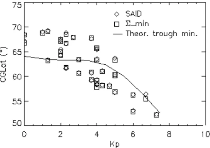
The dependence of the SAID event location and of the cor-responding conductivity minimum position, as well as of the associated trough minimum location, on the magnetic activ-ity was analyzed. Figure 9 shows the position of these fea-tures as a function of the magnetic activity index Kp.

The SAID events location is represented by diamonds, while squares represent the corresponding conductivity min-imum location. Both these features are seen to move towards lower latitudes for increasing Kp value. The solid line

rep-resents the average position of the corresponding theoretical trough minimum. For low Kp values (<3), the majority of

the SAID events is seen to be located poleward of the corre-sponding trough minimum. With increasing magnetic activ-ity, both SAID events and trough minimum positions move towards lower latitudes. However, the majority of the SAID events are now found to be located on the equatorward side of the corresponding trough. This result might indicate that the movement of the SAID location towards lower latitudes with increasing Kp, possibly occurs on a shorter time scale

Fig. 9. Latitudinal variation of both SAID events (diamonds) and

corresponding conductivity minimum (squares) positions versus magnetic activity index Kp. The solid line represents the average position of the corresponding theoretical trough minimum.

In Fig. 10 the spatial average of the net FAC density versus the electric field peak intensity corresponding to the mea-sured SAID events is plotted. For this analysis each orbit data file was divided into three different regions: “event re-gion” – the limits of this region are marked with two green guidelines in the first panel of the previously shown Fig. 6. The distance between these lines is equal to two times the width of the event; “equatorward region” – the region lo-cated between 50◦CGLat and the equatorward limit of the event region; “poleward region” - the region located between the poleward limit of the event region and 70◦CGLat.

The top panel shows the average FAC density distribu-tion corresponding to the equatorward region. Negative val-ues correspond to an average net downward FAC density, while positive values correspond to a net upward FAC den-sity. These definitions are valid for both hemispheres. This plot shows that for the majority of the events, there is a net FAC density flowing downwards in the equatorward region. FAC densities up to 3 µ A/m2were measured with one event reaching a density of approximately 7 µ A/m2. The center panel refers to the event region. In this region there is almost a balance between events with a net downward FAC density and events with a net upward FAC density. In the bottom panel the average net FAC distribution corresponding to the poleward region is plotted. For the majority of the events, the net FAC density flows upwards in this region, showing densities up to 4µ A/m2.

These plots also show that the development of rapid SAID events does not necessarily require intense FAC densities. The majority of the intense FAC densities is associated with electric field peak intensities less than 100 mV/m. Calcu-lations have also shown that for 2/3 of the total number of events, the total net current is upward. For these cases, an average of 20% of the total upward current was not balanced by the downward current.

Fig. 10. Distribution of the average FAC density versus the electric

field peak intensity (Epw) corresponding to three different regions. Top panel: equatorward region; Center panel: event region; Bottom panel: poleward region. Negative (positive) values indicate a net downward (upward) FAC density. These definitions are valid for both hemispheres.

4 Discussion and conclusions

In this statistical study, the SAID events were shown to oc-cur predominantly in the premidnight sector, with a maxi-mum probability within the 20:00 to 23:00 MLT sector. This is in agreement with earlier findings, such as by Spiro et al. (1979), Anderson et al. (1991), Karlsson et al. (1998), Burke et al. (2000), Anderson et al. (2001), and with the model pre-dictions presented by Southwood and Wolf (1978). Accord-ing to their model, SAID events would occur predominantly in the premidnight sector, where the inner edge of the proton ring current extends earthward of the inner edge of the elec-tron ring current. The production mechanism proposed later on by Keyser et al. (1998) also predicted the same result. Due to the relative motion between the hot injected plasma and the plasmaspheric corotation shear velocity at the cold plasma trough interface, which is largest in the premidnight sector, SAID would predominantly occur in this region. This result is also described by the models proposed by Ander-son et al. (1993) and Galperin (2002). Within the 20:00 to 23:00 MLT sector, the most rapid SAID events were also found.

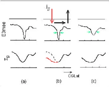
Fig. 11. Schematic picture showing modifications of the reduced

conductivity region (6p) and of the location and intensity of the associated SAID electric field peak (E3mee).

The analysis of the SAID properties with substorm evolu-tion has shown an increase in the electric field peak inten-sity accompanied by a decrease in the corresponding latitu-dinal width, during the initial stage of the related substorm expansion phase. At approximately 30 to 40 min after on-set, the most intense electric fields corresponding to the nar-rowest peaks are detected. During the substorm recovery phase, the SAID structures widen and the electric field in-tensity decreases. The potential drop measured across the SAID events shows an average value of approximately 4 kV during the first 30 min after substorm onset. After this initial stage, the average potential drop decreases to ∼2.5 kV, re-maining then fairly constant during the recovery phase. The anti-correlation observed between the SAID electric field in-tensity and its latitudinal width, which results in a roughly constant potential across the SAID structure during the evo-lution of the substorm, is a feature that would suggest the model of a voltage generator acting as the magnetospheric source for the SAID formation. However, the analysis of the calculated height-integrated Pedersen conductivity pro-files clearly demonstrated that SAID events are associated with a reduction of the ionospheric conductivity, with the most intense electric field peaks being associated with the lowest conductivity minimum values. This feature points, on the other hand, at a magnetospheric current generator as the source for the SAID formation.

These results suggest that the SAID generation mechanism has properties of both a voltage and a current magnetospheric generator. However, since our data set refers only to the iono-spheric end of the SAID flux tube, it is here not possible to reveal the true nature of the SAID generator. Our results have also shown clear ionospheric modifications associated with the SAID occurrence, suggesting that ionospheric feed-back mechanisms are of major importance for sustaining and modifying the SAID structure.

1. The majority of the SAID events (2/3) were found to be located on the poleward side of the associated low conduc-tivity region, with the most intense ones located closer to the conductivity minimum.

2. The reduced conductivity regions associated with the SAID structures show an asymmetric morphology. Typically the equatorward edge is more rounded, whereas the pole-ward edge is more abrupt. The steepest edges were found to be concentrated at the 20:00 to 23:00 MLT sector where the most intense SAID electric fields were also detected.

These results have been discussed in several previous stud-ies based on particle data analysis and also on model pre-dictions. Spiro et al. (1979) reported on a few SAID events and the associated total ion concentration profiles. In all four cases shown, the SAID peak velocity was located near the poleward edge of the associated reduction in the ion concen-tration. For the presented cases, these regions of reduced ion concentration were rounded near the equatorward edges and more abrupt near the poleward edges. This is in accor-dance with the model predictions by Harel et al. (1981a) and Harel et al. (1981b), where the ionospheric currents would flow across a region of low conductivity, generating a peak in the electric field where the conductivity gradient was the sharpest, i.e. on its poleward side. Grebowsky et al. (1978) and Foster et al. (1979) described the SAID events as iono-spheric signatures of the plasmapause, and showed that the equatorial plasmapause was typically located at, or at higher latitudes than the equatorward edge of the ion trough. An-derson et al. (1991) have also shown that in most of the cases where a deep ion trough was seen to be present prior to the SAID formation, the SAID deepened the poleward part of this preexisting trough. According to the generation mech-anism proposed by Keyser (1999), the SAID formation was also predicted to be predominantly located poleward of, or in, the vicinity of the plasmapause.

3. The SAID structure is seen to widen during the course of the substorm recovery phase.

Our interpretation of results 1, 2 and 3 is schematically represented in Fig. 11. The SAID electric field peak is asso-ciated with a reduction of the ionospheric Pedersen conduc-tivity (a). The analysis of the calculated field-aligned cur-rents distribution, Fig. 10, showed that in the equatorward region of the SAID event the FAC flows mainly downwards, whereas in the poleward region the FAC flows mainly up-wards. Since the downward FAC is mainly carried by elec-trons flowing upwards, a depletion of the ionospheric density in the SAID equatorward region occurs, leading to a reduc-tion of the Pedersen conductivity in this region (b). Conse-quently, the SAID electric field peak is located polewards of the corresponding conductivity minimum, and the reduced conductivity region shows a more rounded equatorward edge and a steeper poleward edge. As a consequence of these ionospheric modifications occurring within the SAID region, the SAID structure will also modify and become wider, such that Pedersen currents can flow through the region of low conductivity, and the electric field peak become weaker, such

that the associated potential drop might remain roughly con-stant (c).

4. Figure 9 revealed that SAID events are located rel-atively close to the minimum of the corresponding mid-latitude trough, and that both these features have a similar re-sponse to magnetospheric disturbances but on different time scales.

The SAID location shows a clear tendency to move to-wards lower latitudes with increasing magnetic activity, in accordance with the findings reported by Karlsson et al. (1998) and with the model predictions by Keyser (1999). The location of the corresponding low conductivity region mini-mum is seen to follow the same trend. Also for the corre-sponding mid-latitude trough minimum, as predicted by the Werner and Pr¨olss (1997) empirical model, a similar trend is seen, mainly for high magnetic activity levels. The analy-sis of the relative position of these features for different Kp

values shows that, while for low magnetic activity levels, the SAID is located poleward of the trough minimum, for higher magnetic activity levels, the SAID event is seen to be pre-dominantly formed close to, or equatorwards of, the corre-sponding trough minimum. This result might indicate that the response of the SAID structure to magnetospheric distur-bances occurs on a shorter time scale than the ionospheric trough, which shows a slower movement towards lower lati-tudes with increasing magnetic activity.

A main goal of this study was to improve our understand-ing of the SAID phenomenon and to understand the role of the ionosphere on sustaining and modifying the SAID struc-tures. A key issue in many previous studies of SAID is whether these structures are driven by a voltage or by a cur-rent generator. Our results indicate that the SAID generator has properties of both a current and a voltage magnetospheric generator. Since the analyzed data set corresponds only to the ionospheric end of the SAID flux tube, it is here not possible to determine exactly where on the scale between a pure volt-age generator and a pure current generator the SAID genera-tor would fall. Our results also indicate that the ionospheric feedback mechanisms play a major role in sustaining and regulating the SAID structures. Further studies are required to understand the relevant ionospheric feedback mechanisms involved, how do they act, and how and on which time scale the SAID structure responds to this interaction.

Appendix A Method for FAC density calculation

For the calculation of the FAC densities, the magnetic field data measured by the EMMA instrument was used. Af-ter despinning, the magnetic field data initially recorded in the GEI (Geocentric Equatorial Inertial) coordinate system was optionally converted to the MEE (Magnetic field-East-Equatorward) system. In this reference frame the e1mee

axis is aligned with the background magnetic field direction, e2meepoints eastward and e3meecompletes the triad pointing

equatorwards.

The steady-state relation between current density, j, and the magnetic field, B, is given by Amp`ere’s law:

∇ ×B = µ0j, (A1)

where µ0is the vacuum permeability.

Although a simple relation, applying it on the estima-tion of current density using single spacecraft magnetometer measurements presents some difficulties, since the magnetic field is only known along the satellite orbit and thus, the spa-tial gradient on the other two directions are unknown.

Since at the altitude of the Astrid-2 satellite (∼1000 km), the magnetometer is only sensitive to magnetic field-aligned currents, the contribution of ionospheric currents can thus be neglected, and a field-aligned structure assumed. In this type of study it is common to apply the infinite current sheet ap-proximation and to assume an east-west current sheet align-ment, also known as L-shell alignment.

Fung and Hoffman (1992) presented a study where they questioned the application of the infinite current sheet ap-proximation. They concluded that the FAC densities ob-tained using this approximation, may be affected by an error of less than 10%, as long as the satellite crossing occurs far enough from the ends of the FAC region. In a study by L¨uhr et al. (1996), an algorithm for estimating field-aligned cur-rents from single spacecraft magnetic field measurements, was presented. By applying Amp`ere’s law on the coordi-nate system of the spacecraft velocity and the ambient mag-netic field, the proposed algorithm was suited to the condi-tions encountered by the Freja satellite. By calculating simu-lated current density measurements for some simple models they evaluated the reliability of the applied corrections when step by step each one of the commonly applied assumptions were relaxed. Their results show that for incidence angles of the spacecraft velocity relative to the current sheet nor-mal direction less than 60◦the algorithm results agree rather well with the expected values. By testing the dependence of the results on the relation between thickness and width of the current sheet, they found that the correction factor varies typ-ically between 1 and 2 for any geometry configuration of the current sheet, if the incidence angle is less than 60◦.

In the present analysis we assume that all currents are field-aligned and have an infinite sheet-like structure. Since on mid- and high-latitude orbit passages the spacecraft has a dominant velocity component lying in the plane perpen-dicular to the magnetic field direction, reliable FAC density estimates can be obtained. However, the small-scale FAC sheets successively encountered by the satellite may not al-ways be east-west aligned and may also vary during an orbit passage. In order to determine the principal axis of the dif-ferent current sheets, the data set was divided into 8-s data subsets. For each one of these subsets, the minimum vari-ance analysis (Fung and Hoffman, 1992) was applied, and the corresponding normal direction determined.

By considering a coordinate system defined by the cur-rent sheet principal axis (ez,et,en), where ez is parallel to

current sheet, and enparallel to the current sheet normal

di-rection pointing towards lower latitudes, applying Amp`ere’s law results in jz= − 1 µ0 · ∂Bt ∂sn , (A2)

where Bt is the projection of the horizontal magnetic field

on the current sheet tangential direction and snthe horizontal

space coordinate parallel to the current sheet normal direc-tion. Applying this equation to the discrete magnetic data subsets and specifying the spatial gradient in terms of the spacecraft velocity yields

jz= − 1 µ0 · 1Bt vn·1t , (A3)

where vnis the projection of the horizontal velocity

compo-nent on the current sheet normal direction and 1 stands for the difference between two adjacent subset delimiters. For cases where the satellite track is almost tangent to the cur-rent sheet Eq. (A2) becomes very sensitive to measurement errors. Consequently, no reliable FAC estimate can be done. In our study, no FAC density is calculated for cases where the incidence angle was greater than 60◦_.

Appendix B Method for height-integrated Pedersen conductivity calculation

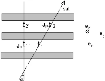
For the introduction of our algorithm, we start by analyzing a simple model where we consider several infinitely large cur-rent sheets, all with the same orientation. Assuming that all downward FACs close with upward going FACs via iono-spheric Pedersen currents flowing along the current sheet normal direction (Fig. B1), the following equation may be written

JP(2’) = JP(1’)±

Z 20 10

jzdsn, (B1)

where the vector JP denotes the Pedersen current. The sign

±corresponds to Northern/Southern Hemispheres and takes into account the fact that in the Northern Hemisphere, a downward field-aligned current assumes a positive value, and in the Southern Hemisphere a negative value, as defined in the (ez,et,en) coordinate system. 1’ and 2’ are arbitrary

points located between different current sheets.

Since the current sheets are assumed to be infinite in length, the Pedersen current vector measured at the satel-lite track point 2 is the same as that measured at point 20. This equality holds for all points having the same coordinate along the current sheet normal axis. Therefore, Eq. (B1) may be applied to the satellite track points (1,2)

JP(2) = JP(1) ±

Z 2

1

jzdsn. (B2)

Expressing the Pedersen current density in terms of the height-integrated Pedersen conductivity, 6P, and the electric

field

JP =6P ·En, (B3)

Fig. B1. Schematic picture of the FAC closure system through the

ionosphere via Pedersen currents. The view is from above the iono-sphere. α is the incidence angle of the spacecraft. 10and 20 are arbitrary points located between different current sheets. 1 and 2 are the corresponding points located along the satellite trajectory.

JP denotes the Pedersen current vector.

and introducing Eq. (A2), Eq. (B2) yields 6P(2) = 6P(1) · En(1) En(2) ∓ 1 µ0 ·Bt(2) − Bt(1) En(2) , (B4)

where En denotes the projection of the horizontal electric

field component on the current sheet normal direction. Since the incidence angle α is determined as described be-fore, and the horizontal electric field, as well as the magnetic field vectors, are measured, the height-integrated Pedersen conductivity in a particular point can be determined, if the height-integrated Pedersen conductivity value of the previ-ous neighbor point is already known. Therefore, once the 6P value is defined for the starting point of the orbital

pas-sage, all the consecutive 6P values can be calculated.

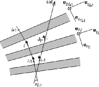
The next step consists of analyzing the model where we consider several infinite current sheets, each one described by a different orientation angle, α0_i(Fig. B2).

Once again, we consider that the Pedersen current flows perpendicularly to the current sheets, along the path resultant from the intersection of the different current sheet normal directions.

Between the points labelled in Fig. B2 asi’-1 and i’ the Pedersen current flows parallel to the direction sn_i0. The same

current density arrived at point i’ flowing parallel to sn_i0, will

now depart towards point i’+1, flowing along the direction sn_i0+1. Therefore, generalizing Eq. (B1) yields

JP(i’) = JP(i’-1) ±

Z i0

i0₋₁

jzdsn_i0. (B5)

Again, assuming a homogeneous Pedersen current den-sity distribution along the current sheet tangential direction,

Fig. B2. Set of non-parallel infinite current sheets (schematic

pic-ture). Again, the view is from above the ionosphere and α_i0 is the

incidence angle of the spacecraft with the current sheet i’. i0−1 and i0are arbitrary points located between different current sheets.

i−1 and i are the corresponding points located along the satellite trajectory. JP denotes the Pedersen current vector.

results in the following expression for the height-integrated Pedersen conductivity value at the satellite track point i 6P(i) = 6P(i-1) · Eni(i-1) Eni(i) ∓ 1 µ0 · Bti(i) − Bti(i-1) Eni(i) . (B6) As mentioned before, it is necessary to define the conduc-tivity value for a starting point of the calculations. In this study we have defined the starting point as the orbit’s passage most equatorward point where two conditions were fulfilled: the variation of the electric field component Enin a interval

of 1 s of data (corresponding to approximately 7 km of dis-tance) is greater than 0.32 mV/m (equivalent to an average variation of 0.2 mV/m between two consecutive data points); the ratio ∓_µ1

0·

1Bt

1En is less than 10 S. Under these conditions, and assuming an uniform conductivity distribution over this region, using Eq. (B6), we derive the expression

6P(st art−point ) = ∓ 1 µ0 · 1Bt 1En , (B7)

where 1 stands for the difference between two neighbor points.

To ensure the reliability of the results obtained with this method, some quality criteria were defined. Using the ob-tained starting point value, the calculation process (Eq. (B6)) evolves until it encountered a point where one or both of the following conditions are not fulfilled: |En|is less than

5 mV/m and/or the resultant 6P value is negative. In this

situation the process stops and a new intermediate starting point is required to continue the calculation. This value is again obtained, making use of Eq. (B7) whenever the corre-sponding required conditions are satisfied.

Acknowledgements. S. Figueiredo acknowledges the support of the

Fundac¸˜ao para a Ciˆencia e a Tecnologia (FCT) under the grant SFRH/BD/6211/2001.

Topical Editor T. Pulkkinen thanks two referees for their help in evaluating this paper.

References

Anderson, P. C., Heelis, R. A., and Hanson, W. B.: The ionospheric signatures of rapid subauroral ion drifts, J. Geophys. Res., 96, 5785–5792, 1991.

Anderson, P. C., Hanson, W. B., Heelis, R. A., Craven, J. D., Baker, N. D., and Frank, L. A.: A proposed production model of rapid subauroal ion drifts and their relation to substorm evolution, J. Geophys. Res., 98, 6069–6078, 1993.

Anderson, P. C., Carpenter, D. L., Tsuruda, K., Mukai, T., and Rich, Multisatellite observations of rapid subauroral ion drifts (SAID), J. Geophys. Res., 106, 29 585–29 599, 2001.

Banks, P. M. and Yasuhara, F.: Electric fields and conductivity in the nighttime E-region: a new magnetosphere-ionosphere-atmosphere coupling effect, Geophys. Res. Lett., 5, 1047–1050, 1978.

Blomberg, L. G., Marklund, G. T., Lindqvist, P.-A., and Bylander, L.: Astrid-2: an advanced auroral microprobe, in “Microsatel-lites as Research Tools”, COSPAR Colloquia Series Volume 10, Elsevier, 10, 57–65, 1999.

Burke, W. J., Rubin, A. G., Maynard, N. C., Gentile, L. C., Sultan, P. J., Rich, F. J., de La Beaujardire, O., Huang, C. Y., and Wilson, G. R.: Ionospheric disturbances observed by DMSP at middle to low latitudes during the magnetic storm of June 4–6, 1991, J. Geophys. Res., 105, 18,391–18,405, 2000.

Foster, J. C., Park, C. G., Brace, L. H., Burrows, J. R., Hoffman, J. H., Maier, E. J., and Whittaker, J. H.: Plasmapause signa-tures in the ionosphere and magnetosphere, J. Geophys. Res., 83, 1175–1182, 1979.

Fung, S. F. and Hoffman, R. A.: Finite geometry effects of field-aligned currents, J. Geophys. Res., 97, 8569–8579, 1992. Galperin, Y. I., Polarization Jet: characteristics and a model, Ann.

Geophys., 20, 391–404, 2002.

Galperin, Y. I., Ponomarov, Y. N., and Zosinova, A. G.: Direct mea-surements of ion drift velocity in the upper ionosphere during a magnetic storm, Kosm. Issled., 11, 273–282, 1973.

Galperin, Y. I., Soloviev, V. S., Torkar, K., Foster, J. C., and Veselov, M. V., Predicting plasmaspheric radial density profiles, J. Geo-phys. Res., 102, 2079–2091, 1997.

Grebowsky, J. M., Hoffman, J. H., and Maynard, N. C.: Iono-spheric and magnetoIono-spheric “plasmapauses”, Planet. Space Sci., 26, 651–660, 1978.

Harel, M., Wolf, R. A., Reiff, P. H., Spiro, R. W., Burke, W. J., Rich, F. J., and Smiddy, M.: Quantitative simulation of a mag-netospheric substorm, 1. Model logic and overview, J. Geophys. Res., 86, 2217–2241, 1981a.

Harel, M., Wolf, R. A., Spiro, R. W., Reiff, P. H., Chen, C.-K., Burke, W. J., Rich, F. J., and Smiddy, M.: Quantitative simula-tion of a magnetospheric substorm, 2. Comparisons with obser-vations, J. Geophys. Res., 86, 2242–2260, 1981b.

Heelis, R. A., Spiro, R. A., Hanson, W. B., and Burch, J. L.: Magne-tosphere ionosphere coupling in the mid-latitude trough, Trans. Am. Geophys. Union, 57, 990–991, 1976.

Karlsson, T., Marklund, G. T., Blomberg, L. G., and Mlkki, A.: Subauroral electric fields observed by the Freja satellite: A

sta-tistical study, J. Geophys. Res., 103, 4327–4341, 1998.

Keyser, J. D.: Formation and evolution of subauroral ion drifts in the course of a substrom, J. Geophys. Res., 104, 12,339–12,349, 1999.

Keyser, J. D., Roth, M., and Lemaire, J.: The magnetospheric driver of subauroral ion drifts, Geophys. Res. Lett., 25, 1625–1628, 1998.

Khalipov, V. L., Galperin, Y. I., Stepanov, A. E., and Shestakova, L. V.: Formation of polarisation jet during substorm expansion phase: Results of ground-based measurements, Cosmic Res., 39, 2001.

L¨uhr, H., Warnecke, J. F., and Rother, M. K. A: An algorithm for estimating field-aligned currents from single spacecraft magnetic field measurements: a diagnostic tool applied to Freja satellite data, IEEE Transactions on Geoscience and Remote Sensing, 34, 1369–1376, 1996.

Maynard, N. C.: On large poleward-directed electric fields at sub-auroral latitudes, Geophys. Res. Lett., 5, 617–618, 1978. Maynard, N. C., Aggson, T. L., and Heppner, J. P.: Magnetospheric

observations of large sub-auroral electric fields, Geophys. Res. Lett., 7, 881–884, 1980.

Rich, F. J., Burke, W. J., Kelley, M. C., and Smiddy, M.: Observa-tions of field-aligned currents in association with strong convec-tion electric fields at subauroral latitudes, J. Geophys. Res., 85, 2335–2340, 1980.

Rodger, A. S., Moffett, R. J., and Quegan, S.: The role of ion drift in the formation of ionisation troughs in the mid- and high-latitude ionosphere - a review, J. Atmos. Terr. Phys., 54, 1–30, 1992. Schunk, R. W. and Banks, P. M.: Effects of electric fields and other

processes upon the nighttime high-latitude F layer, J. Geophys. Res., 81, 3271–3282, 1976.

Smiddy, M., Kelley, M. C., Burke, W., Rich, F., Sagalyn, R., Schu-man, B., Hays, R., and Lai, S.: Intense poleward-directed electric fields near the ionospheric projection of the plasmapause, Geo-phys. Res. Lett., 4, 543–546, 1977.

Southwood, D. J. and Wolf, R. A.: An assessment of the role of pre-cipitation in magnetospheric convection, J. Geophys. Res., 83, 5227–5232, 1978.

Spiro, R. W., Heelis, R. H., and Hanson, W. B.: Rapid sub-auroral ion drifts observed by Atmospheric Explorer C, Geophys. Res. Lett., 6, 657–660, 1979.

Werner, S. and Pr¨olss, G. W.: The position of the ionospheric trough as a function of local time and magnetic activity, Adv. Space Res., 20, 1717–1722, 1997.