HAL Id: hal-00459974
https://hal.archives-ouvertes.fr/hal-00459974
Submitted on 23 Apr 2016
HAL is a multi-disciplinary open access
archive for the deposit and dissemination of
sci-entific research documents, whether they are
pub-lished or not. The documents may come from
teaching and research institutions in France or
abroad, or from public or private research centers.
L’archive ouverte pluridisciplinaire HAL, est
destinée au dépôt et à la diffusion de documents
scientifiques de niveau recherche, publiés ou non,
émanant des établissements d’enseignement et de
recherche français ou étrangers, des laboratoires
publics ou privés.
Satellite monitoring of ammonia: A case study of the
San Joaquin Valley
Lieven Clarisse, Mark W. Shephard, Frank Dentener, Daniel Hurtmans, Karen
Cady-Pereira, Federico Karagulian, Martin van Damme, Cathy Clerbaux,
Pierre-François Coheur
To cite this version:
Lieven Clarisse, Mark W. Shephard, Frank Dentener, Daniel Hurtmans, Karen Cady-Pereira, et
al..
Satellite monitoring of ammonia: A case study of the San Joaquin Valley.
Journal of
Geophysical Research: Atmospheres, American Geophysical Union, 2010, 115 (D13), pp.D13302.
�10.1029/2009JD013291�. �hal-00459974�
for Full Article
Satellite monitoring of ammonia: A case study
of the San Joaquin Valley
Lieven Clarisse,
1Mark W. Shephard,
2Frank Dentener,
3Daniel Hurtmans,
1Karen Cady
‐Pereira,
2Federico Karagulian,
1Martin Van Damme,
1Cathy Clerbaux,
1,4and Pierre
‐François Coheur
1Received 28 September 2009; revised 4 February 2010; accepted 19 February 2010; published 10 July 2010.
[1]
Atmospheric ammonia (NH
3) has recently been observed with infrared sounders from
space. Here we present 1 year of detailed bidaily satellite retrievals with the Infrared
Atmospheric Sounding Interferometer and some retrievals of the Tropospheric Emission
Spectrometer over the San Joaquin Valley, California, a highly polluted agricultural
production region. Several sensitivity issues are discussed related to the sounding of
ammonia, in terms of degrees of freedom, averaging kernels, and altitude of maximum
sensitivity and in relation to thermal contrast and concentration. We also discuss their
seasonal dependence and sources of errors. We demonstrate boundary layer sensitivity
of infrared sounders when there is a large thermal contrast between the surface and the
bottom of the atmosphere. For the San Joaquin Valley, large thermal contrast is the case for
daytime measurements in spring, summer, and autumn and for nighttime measurements in
autumn and winter when a large negative thermal contrast is amplified by temperature
inversion.
Citation: Clarisse, L., M. W. Shephard, F. Dentener, D. Hurtmans, K. Cady‐Pereira, F. Karagulian, M. Van Damme, C. Clerbaux, and P.‐F. Coheur (2010), Satellite monitoring of ammonia: A case study of the San Joaquin Valley, J. Geophys. Res., 115, D13302, doi:10.1029/2009JD013291.
1.
Introduction
[2] The presence of atmospheric ammonia (NH3) made
first life on Earth possible [Wigley and Brimblecombe, 1981]. Today, ammonia sustains life as a major component in the global nitrogen cycle, with over 40% of the population owing their life to the industrial synthesis of ammonia via the Haber‐ Bosch process [Erisman et al., 2007; Smil, 2002]. Agriculture as a whole is responsible for the majority of the global atmospheric emissions of ammonia; for example, in the United States and Europe about 80% of all emissions are related to agriculture. Other emissions include those from biomass burning and natural sources such as the release from the oceans and vegetation. Emissions have increased con-siderably since pre‐industrial times and are unlikely to go down because of the ever growing demand for food and feed [Galloway et al., 2004; Aneja et al., 2008; Sutton et al., 2008]. As the primary base and primary form of reduced nitrogen in the atmosphere, elevated amounts of ammonia have a wide range of environmental effects such as deposition of reactive
nitrogen in sensitive ecosystems and enhanced creation of particulate matter [Bauer et al., 2007; Cowling and Galloway, 2002; Galloway et al., 2003; Krupa, 2003].
[3] Despite its importance, ammonia is one of the most
poorly quantified trace gases, with errors over 50% on the global emission budget and even higher on temporal and local scales [Dentener and Crutzen, 1994; Matthews, 1994; Bouwman et al., 1997; Pinder et al., 2006; Sutton et al., 2007; Faulkner and Shaw, 2008; Galloway et al., 2008; Sutton et al., 2008; Reis et al., 2009]. In Europe, the United States and Asia, there are a limited number of routine ammonia observations of NH3. In Europe EMEP (http://tarantula.nilu.
no/projects/ccc/network/) operates about 20 sites of mostly filterpack measurements, while in the United States, NADP (http://nadp.sws.uiuc.edu/nh3Net/) started recently a net-work consisting of 21 passive samplers. EAnet (http://www. eanet.cc/) in Asia uses passive samplers to measure surface ammonia at about 25 sites. It is, however, challenging to capture the temporal and spatial variability of ammonia using such sparse ground‐based measurements alone, as ammonia (gas phase) is very reactive with a tropospheric lifetime not more than a few hours. Beyond the limited set of direct sur-face measurements, NH3concentrations can be explored with
total wet NHxmeasurements [Gilliland et al., 2003, 2006] or
using the balance of particulate sulfate and nitrate coupled with inverse modeling [Henze et al., 2009]. Space measure-ments may also complement surface observations by pro-viding high spatial coverage, as for instance in the infrared sounding of species as CO, CH4, O3, HNO3and volcanic SO2
[Clerbaux et al., 2009]. 1Spectroscopie de l’Atmosphère, Service de Chimie Quantique et
Photophysique, Université Libre de Bruxelles, Brussels, Belgium.
2
Atmospheric and Environmental Research, Inc., Lexington, Massachusetts, USA.
3
European Commission, Joint Research Centre, Ispra, Italy.
4Université Paris 06, Université Versailles St.‐Quentin, CNRS, INSU,
LATMOS‐IPSL, Paris, France.
Copyright 2010 by the American Geophysical Union. 0148‐0227/10/2009JD013291
[4] First measurements of ammonia from space were
reported over the Beijing and San Diego area with the Tro-pospheric Emission Spectrometer (TES) [Beer et al., 2008] and in biomass burning plumes with the Infrared Atmo-spheric Sounding Interferometer (IASI) [Coheur et al., 2009] satellite. Later, exploiting IASI’s spatial and temporal reso-lution, a first global map of ammonia was obtained by cor-relating observed brightness temperature differences to total columns [Clarisse et al., 2009]. Using this approach, it was concluded that there are likely underestimates of global emission inventories at a number of NH3hot spot regions.
These hot spot regions were often found in valleys with substantial agricultural production, such as the Po Valley in Italy, the Fergana Valley in Uzbekistan and the San Joaquin Valley (SJV) in the United States. In this paper we study detailed retrievals of ammonia concentrations from infrared spectra measured above the SJV. There are a number of reasons why ammonia is important in the SJV and why it is a good test case for infrared retrievals from space. They are as follows.
[5] 1. From the global measured distributions [Clarisse
et al., 2009] the SJV was found to have the largest abun-dances in the world with a yearly daily average value over
3 mg/m2 (for which the TM5 global model using the
Bouwman emission inventory gives columns below 1 mg/m2
[Bouwman et al., 2002; Dentener et al., 2006]).
[6] 2. The National Ambient Air Quality Standards
(NAAQS) are frequently violated in the SJV [Hall et al., 2008]. For ozone and fine particulate matter (PM2.5) stan-dards, the EPA classifies the valley as a nonattainment area with some of the worst pollution in the United States [U.S. Environmental Protection Agency, 2008; Hall et al., 2008; Pun et al., 2009; Ying and Kleeman, 2009; Kleeman et al., 2005] (see also U.S. Environmental Protection Agency, The green book nonattainment areas for criteria pollutants, 2009, http://epa.gov/oar/oaqps/greenbk/). Ammonia plays an important role in the formation of particulate matter [U.S. Environmental Protection Agency, 2008; Anderson et al., 2003], with ammonium sulphate and ammonium nitrate accounting each between 20% and 30% of the total mass of fine matter on an average annual basis in the San Joaquin Valley [Chow et al., 2006; Malm et al., 2004; Ying and Kleeman, 2006]. Ammonia emitted in the San Joaquin Valley is also transported to the Sierra Nevada, where it may severely affect the forest ecosystems [Bytnerowicz et al., 2002; Hunsaker et al., 2007].
[7] 3. EPA has not defined a NAAQS for ammonia, but
emissions in the SJV are known to rank among the highest in the United States [Goebes et al., 2003; Pinder et al., 2003; Makar et al., 2009] (see also U.S. Environmental Protection Agency, County emissions map: Criteria air pollutants, 2008, http://www.epa.gov/air/data/emisdist.html?us USA United States). A 2003 estimate attributes 64.1% of the emissions in the San Joaquin Valley to livestock, 13.5% to motor vehicles, 11.7% to fertilizers, 6.3% to vegetation [Battye et al., 2003]. In terms of cash farm receipts, California is the largest state of the United States, with $36.6 billion in revenue representing 12.8% of the national total (17.8% in crops and 7.8% in livestock). The majority of this comes from the San Joaquin Valley, principally from grapes, nuts, citrus, tomatoes, dairy products, chickens, cattle and calves (California Department of Food and Agriculture, California Agricultural Resource
Directory 2008–2009, http://www.cdfa.ca.gov/statistics/). Although there have been a few ground‐based measurements of ammonia in the SJV [Lunden et al., 2003; Ying et al., 2008; Zwicker et al., 1998] during the winter months, it is surpris-ingly not being monitored as part of the national ammonia network. While in Europe emission control policies, careful monitoring and the introduction of new technologies have lead to a 40% reduction in emissions since 1995, emissions in the United States are still on the increase [Reis et al., 2009; Aneja et al., 2008]. Reducing ammonia emissions in the SJV will be a real challenge as agriculture is likely to remain very intensive in this region.
[8] 4. Other contributing factors to the pollution of the
valley are the warm and dry climate and the topography of the valley which hampers vertical mixing and allows buildup of pollutants [Hall et al., 2008; Ying et al., 2008]. In the fall and winter the high‐pressure field of the Pacific Ocean leads to subsiding hot air, which favors clear skies and strong radia-tive cooling at night. The hot air can act as a lid over the valley, creating a temperature inversion layer which traps cool moist air below [Holets and Swanson, 1981; Jacob, 1999; Herckes et al., 2007]. In this case the temperature of the surface can be much cooler than the air above. This is what we will call a negative thermal contrast. In general thermal contrast can be defined as the temperature difference between the surface and the air temperature at some altitude of inter-est (for ammonia this will be in the boundary layer). In spring, summer and autumn daytime the thermal contrast can be as large as 20 K. In the evening and at night it is usually very small, except at certain periods of the year or in case of temperature inversion, which frequently occurs over the SJV. This wide variety of thermal conditions, from high to low thermal contrast and possible temperature inversion at night, is interesting from a remote sensing point a view, as thermal contrast influences the sensitivity of the satellite IR mea-surements to the boundary layer (and therefore our ability to sense ammonia).
[9] The spectra used in our analysis were taken mainly
from IASI observations, which combines a good spectral resolution and radiometric noise with bidaily global cover-age. As we have analyzed a whole year of IASI spectra, it was possible to find some colocated measurements of the TES instrument, and we use the opportunity to discuss and com-pare some retrievals from TES. TES does not have frequent spatial coverage but combines good radiometric noise with a high spectral resolution and a favorable overpass time at 1330 local solar time. We will use it to make a first assessment of the impact of spectral resolution on the retrievals. In section 2 we describe the IASI and TES instruments and explain the choice of a priori and covariance matrix selected for the retrievals. We present three sample retrievals from spectra measured under different conditions in section 3. We dem-onstrate that, depending on the thermal contrast and specific temperature profile, it is possible to sense down to the boundary layer and show that temperature inversion in the SJV also allows for accurate retrievals from nighttime spectra. We show this independently in section 4, where we present a series of forward simulations to demonstrate the altitude dependency of the observed signal to the thermal contrast. In section 5 we present the results of one complete year of retrievals, analyzing the statistical robustness (expressed as the degrees of freedom), altitude of maximum sensitivity
CLARISSE ET AL.: MONITORING AMMONIA WITH SATELLITES D13302 D13302
and averaging kernels as a function of thermal contrast. We also discuss the main sources of errors in the retrieval of the concentrations. In section 6 we present our conclusions and formulate recommendations for future research.
2.
Sounders and Retrieval Method
[10] The MetOp‐A platform with IASI on board was
launched in a Sun‐synchronous orbit around the Earth at the end of 2006. The overpass times are 0930 and 2130 mean local solar time. Combining the satellite track with a swath of 2200 km, IASI provides global coverage of the Earth twice a day with a footprint of 12 km in nadir modus. The Fourier transform spectrometer IASI measures the thermal infrared radiation emitted by the Earth’s surface and atmosphere in the range 645–2760 cm−1with a spectral resolution of 0.5 cm−1
apodized and noise between 0.15 K and 0.2 K at 950 cm−1and 280 K. IASI’s primary goal is aiding numerical weather prediction, principally by providing temperature and humid-ity profiles. Preliminary validation shows retrieval errors to be lower than 10% for the humidity profiles. For the tem-perature profiles, the error bar is on the order of 1.5–2 K at the surface and in the upper troposphere and 0.6 K in the free troposphere [Pougatchev et al., 2009]. For this case study we used the calibrated radiance spectra and meteorological products consisting of pressure, temperature and humidity profiles, surface temperature and cloud coverage as distrib-uted by EUMETCast near‐real‐time service. The processed spectra were taken from 2008 and selected within 36.25 ± 1° latitude and−119.35 ± 1° longitude, selecting surface altitude below 750 m above sea level and cloud coverage below 10%. This rectangle covers a large part of the SJV and contains Fresno, its largest city.
[11] The Fourier transform spectrometer TES is one of the
instruments on board the AURA satellite [Schoeberl et al., 2006] which was launched in July 2004 in a Sun‐synchronous orbit around the Earth with local overpass times at 0130 and 1330 mean solar time. TES is an interferometric spectral
radiometer and its measured nadir spectra have 0.06 cm−1
unapodized spectral resolution and footprints of 8 × 5 km2 resulting from the averages of 16 element detector arrays where each detector has a 0.5 × 5 km2nadir footprint. TES has a number of observational modes (e.g., global survey, step and stare, transect). In global survey mode TES makes mea-surements along the satellite track for 16 orbits with a spacing of 182 km; in step‐and‐stare mode, nadir measurements are made every 40 km along the track for approximately 50° of latitude; in transect mode observations consist of series of 40 consecutive scans spaced 12 km apart providing a coverage that is much more dense than the routine TES Global Survey viewing mode. The thermal infrared is covered in four spec-tral bands for which we used the 1B2 band (923–1160 cm−1).
The radiometric noise lies between 0.15 K and 0.2 K at 950 cm−1 and 280 K, similar to that of IASI [Worden et al., 2006]. We also used the surface temperature and vertical distributions of atmospheric temperature and H2O which are retrieved
oper-ationally [Shephard et al., 2008a; Bowman et al., 2006; Shephard et al., 2008b].
[12] For the retrieval of ammonia and interfering trace
gases we used the optimal estimation method, basically fitting a calculated spectrum to an observed spectrum, by controlled variation of atmospheric parameters (such as the
concentra-tion of ammonia). We have used the optimal estimaconcentra-tion method as implemented in the program Atmosphit, for which the details are described elsewhere [Rodgers, 2000; Clarisse et al., 2008; Coheur et al., 2005]. The retrieval range was set at 940–969 cm−1which contains the strongest absorption
lines of the n2 band of ammonia. Ammonia along with
interfering H2O were fitted in 10 partial columns of 1 km
thickness, from 0 km to 10 km. Optimal estimation requires an a priori which represents the best possible knowledge of the different parameters prior to retrieval from the spectrum. Alongside the a priori it also needs a covariance matrix, representing the expected variability and correlations between the different parameters. Very little is known about atmo-spheric profiles of ammonia, and as far the measurement of atmospheric columns is concerned, we are only aware of one published experiment [Murcray et al., 1989]. The a priori and covariance matrix for ammonia were therefore calculated
from vertical NH3 profiles computed by the TM5 global
model with the Bouwman emission inventory [Bouwman et al., 2002; Dentener et al., 2006]. Due to the spatial var-iability of ammonia, a global a priori and covariance matrix is not appropriate, as, for example, the magnitude and var-iability of emissions from oceans is quite different from agricultural emissions. Similar to the method presented by M. Shephard et al. (TES ammonia retrievals: Retrieval strategy and initial comparisons, manuscript in preparation, 2010), monthly profiles of the model output were divided in two bins, one with profiles having surface concentrations below 5 ppb and one with concentrations above this, representing moderately polluted and polluted situations, respectively. Figure 1 shows the a priori for both bins and the covariance matrix of the polluted profile. Note that the covariance matrix is dimensionless as it was obtained from the normalized profiles (dividing all polluted and moderately polluted profiles by the average polluted or moderately polluted profile). The altitudes are shown here with respect to the altitude of the surface. Off‐diagonal elements repre-sent correlations between different altitudes, whereas diag-onal elements represent expected variability around the mean. Expected variabilities range from 200% to 500% around 3 km, corresponding to outflow from the boundary
layer. As ground‐based measurements in the SJV report
surface concentrations typically higher than 10 ppb, with peaks up to 150 ppb [Lunden et al., 2003; Ying et al., 2008; Zwicker et al., 1998], the use of polluted profile and covariance matrix for the retrievals is indeed justified. We note that the real vertical ammonia profile can vary with, for example, mixing heights and availability of unneutralized sulfate. We justify the use of a single polluted and moderately polluted profile with the fact that the model profiles are very uncertain, and the traceability of the impact of the a priori profile is more straightforward with only two types of pro-files. We return to this issue in section 5. In section 3, three sample cases are chosen to illustrate the retrieval with this set of constraints.
3.
Sample Retrievals
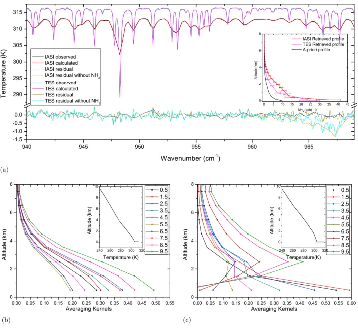
3.1. Positive Thermal Contrast
[13] The first spectra are taken from the IASI and TES
morning orbits of 25 July, a typical hot summer’s day and the IASI and TES spectra were chosen as to coincide
geo-graphically as close as possible (around 36.32° latitude and −119.65° longitude). We recall that there is also a lag of 4 h between the TES and IASI retrievals. Figure 2a shows the observed and fitted spectrum for both TES and IASI and the residuals (difference between observed and calculated spec-trum). The residuals average well below 0.2 K, within the expected noise of the spectrometers. Also shown are the respective residuals with ammonia excluded from the radia-tive transfer calculations. They both have minimum values
around 1.3 K at 967 cm−1pointing to a very high ammonia
content. The fact that they both have approximately the same 1.3 K is rather coincidental, and should not be expected in general, given the different spectral and horizontal resolution and overpass times. The retrieved profiles are shown in an inset and correspond to total columns of 6.8 ± 1.1 · 1016and
4.76 ± 1.1 · 1016 molecules NH3 per cm
2
, with ammonia concentrations at the surface of 34.69 ± 6.43 and 24.46 ± 5.41 ppb of IASI and TES, respectively. Keeping in mind that this is just one example, it is somewhat surprising that the ammonia columns were found higher in the morning (IASI) than at noon (TES) given the temperature dependence of ammonia volatilization. Indeed, Ying et al. [2008] report diurnal peaks in the SJV during winter between 1000 and 1600 local solar time. Ammonia concentrations peaking at night or in the morning are however not uncommon (see, e.g., Walker et al. [2004], Hu et al. [2008] and section 5) and one should keep in mind the extreme volatile character of ammonia (diurnal variants up to a factor five were reported by Ying et al. [2008]) and the fact that IASI and TES have a different pixel size.
[14] Figures 2b and 2c show for the two retrievals the
corresponding averaging kernels for the ten retrieved partial columns. For almost all levels most of the information is
derived from the lowest layer (0 km to 1 km) as this is where the averaging kernels peak. Thus both sounders probe the atmosphere down to the surface in this example. This is a direct consequence of the high thermal contrast between the surface and the surface air temperature (it is 8.5 K at the time of the IASI overpass and 12.3 K for the TES overpass; see Figure 2 insets) and the a priori profile of ammonia which also peaks at the surface. The trace of the averaging kernel matrix, the so called degrees of freedom of the signal (DOFS) is indicative of the information content in the retrieval, and is here for the IASI spectrum 1.007 and for the TES spectrum 1.316. So in total about 1 partial column was extracted from the spectra. Because of the better spectral resolution, the DOFS is usually somewhat higher for the TES retrieval, as is revealed here with a secondary peak in the averaging kernel at 2.5 km. This would in principle allow separating to some extent the ammonia concentration in the boundary layer from that in the free troposphere. For both spectra, the averaging kernel of the retrieved concentration between 0 and 1 km peak at the right altitude with values of 0.29 for IASI and 0.54 for TES, suggesting higher surface sensitivity for the latter. The difference is again due to the higher spectral resolution of TES and the higher thermal contrast at the overpass time of TES. Note that the present example is not a“best case sce-nario,” with only moderately high thermal contrasts (8.5 K and 12.3 K). Higher thermal contrasts up to 20 K were com-monly observed in the San Joaquin Valley (see section 5), improving the surface sensitivity for both sounders.
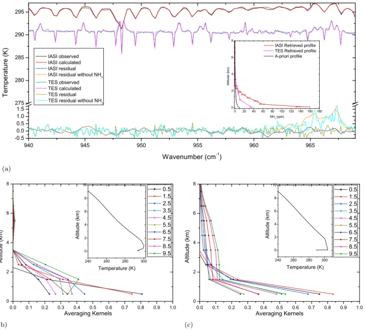
3.2. Negative Thermal Contrast
[15] The second example is one of negative thermal
con-trast, mostly due to the presence of a temperature inversion layer at a few hundred meters altitude. The spectra were Figure 1. (a) A priori moderately polluted (blue) and polluted (red) profile of ammonia. (b) Covariance
matrix of the polluted profile (dimensionless).
CLARISSE ET AL.: MONITORING AMMONIA WITH SATELLITES D13302 D13302
observed on the evening and night of 6 September, around 36.03° latitude and−119.42° longitude. Figure 3 summarizes the retrievals. The features in the spectrum and residuals are comparable to the previous example, except for the fact that this time not absorption but instead emission features are
observed reaching 1.6 K around 967 cm−1. For the IASI
spectrum, the thermal contrast between the surface and the air at the surface is close to 0, with a surface temperature and surface air temperature around 295 K. The TES temperature profile in Figure 3c shows a surface temperature of 289 K and surface air temperatures of 304 K. The reported surface air temperatures from TES and IASI do not seem to be consis-tent, especially considering the fact that the overpass time of
TES is in the middle of the night and the fact that IASI, with an overpass time 4 h earlier, measured an air surface tem-perature 10 degrees colder. Indeed, local weather measure-ments report air temperatures of 300.95 K at the IASI overpass time and 296 K at the TES overpass time (http:// raws.wrh.noaa.gov/cgi‐bin/roman/meso_base_past.cgi? month1=09&day1=6&year1=2008&unit=1&hour1=9& time=GMT&stn=KFAT). If we assume that these local air temperatures are representative for the observed pixel, it would indicate errors in surface air temperature profile of 6 K for IASI (underestimation) and 8 K for TES (overestimation). Having an erroneous temperature profile, can result in large errors in the retrieval, which we will discuss in section 5.3. Figure 2. Retrieval summary of spectra with high thermal contrast. (a) Observed and fitted spectra and
residuals (all in brightness temperatures) and retrieved NH3profiles (ppb) (inset) for both a TES and IASI
spectrum. A residue for a retrieval without ammonia is also shown. (b) Averaging kernels and temperature profiles (kelvins) (inset) of IASI. A surface temperature of 313 K has been indicated. The labels 0.5 to 9.5 are representative for the retrieved columns 0–1 km to 9–10 km. (c) Averaging kernels and temperature profiles (inset) of TES. A surface temperature of 317 K has been indicated. The DOFS equal 1.007 and 1.316 for IASI and TES, respectively.
We did not attempt to make any correction here, as with the surface air temperature, the whole temperature profile would have to be adjusted. When taking a closer look at the IASI temperature profile we note that the temperature increases to about 300.2 K at 800 m pointing to a clear inversion layer,
corresponding to a maximal thermal contrast of −5 K. For
TES the temperature profile in the boundary layer is much straighter at around 304 K, corresponding to a maximum thermal contrast of−15 K.
[16] The retrieval resulted for IASI in a total column of
1.85 ± 0.52 · 1017 molecules NH3per cm2with a surface
concentration of 144 ± 15 ppb and a DOFS of 1.26. For TES the retrieved total column is 0.75 ± 0.11 · 1017molecules NH3per cm2with a surface concentration of 35 ± 2 ppb and a
DOFS of 1.17. As IASI is likely underestimating the surface air temperature, the inversion layer is underestimated, and more ammonia is needed to account for the emission lines. So the IASI retrieved columns are in this case likely
over-estimated. Analogously, in this example the TES retrievals must be underestimated, if indeed the thermal contrast is overestimated. Most importantly again, the averaging kernels indicate a large sensitivity to concentrations in the boundary layer, with small error bars near the surface (not incorporating the erroneous temperature profiles), see Figures 3b and 3c. Although the DOFS of the IASI spectrum is a little higher than TES for this example, it is usually the other way around with maximum values for IASI of 1.5 and for TES of 2. Note that these values are typically higher than for a case with high positive thermal contrast. The reason for this is that an inversion layer is often localized in space (e.g., from the surface up to 1 km altitude), so that when the spectrum shows emission lines, these must be emitted from within that altitude range. In other words, emission lines point exactly to the region where the emitting ammonia is located.
Figure 3. Same as Figure 2 but with high negative thermal contrast. Surface temperatures of 289 K and 295 K have been indicated for TES and IASI, respectively. The DOFS equal 1.26 and 1.17 for IASI and TES, respectively.
CLARISSE ET AL.: MONITORING AMMONIA WITH SATELLITES D13302 D13302
3.3. Low Thermal Contrast
[17] In this third example, we discuss a low thermal
con-trast condition, typical for daytime winter months. We chose a spectrum in the morning orbit of IASI on 20 November. We were unable to match an IASI spectrum with a TES spectrum for this period. For the target area in 2008, just 20 TES spec-tra were observed in total during the months November, December, January, February and March of which all of them either cloudy, located on higher altitude or observed during night. Figure 4 summarizes the retrieval for IASI under the low thermal contrast conditions. The IASI spectrum, fit and residue (not shown here) are very similar to the first example, except a weaker signal in the residue of 0.64 K. Although the ammonia signal is clearly visible in the analyzed residual, because of lower thermal contrast, most of the signal comes from layers above the boundary layer. This can be seen from the averaging kernels which peak at 2.5 km. The limited sensitivity to the boundary layer concentration results in large error bars, peaking at 70% near the surface. The lowest error bar is at 3.2 km at around 35%, for higher altitudes error bars are relative larger again. This particular example illustrates well that a total column is often not the best way to quantify ammonia, as the error on the total column is determined by the lowest levels, which in this case was found to be 3.9 ± 2.3 · 1016molecules NH3per cm2. The large error bar is also
reflected in a relative low DOFS of 0.87.
4.
Boundary Layer Sensitivity
[18] Infrared sounders are often said to have limited or
no sensitivity to the bottom of the atmosphere. This is overly
simplistic, and in general will depend on the target species, thermal contrast, instrumental noise and spectral resolution. We have demonstrated in section 3 that in favorable
con-ditions, the averaging kernels associated with the NH3
retrievals peak at the bottom of the atmosphere. However, retrieval methods vary and averaging kernels depend on the choice of covariance matrix. In this section we will demon-strate this boundary layer sensitivity using the forward model only, independent of any retrieval method, covariance matrix or calculation of derivatives.
[19] For the sensitivity study we have simulated 220
dif-ferent spectra varying the temperature of the surface (and thereby the thermal contrast) using either a typical day or typical night profile and either an moderately polluted or polluted concentration profile of ammonia. For the profiles we have normalized the moderately polluted a priori profile to have surface concentrations of 5 ppb and the polluted a priori profile to have surface concentrations of 20 ppb. The spectra
were simulated at the IASI sampling of 0.25 cm−1between
900 and 1000 cm−1 and convoluted with the IASI
instru-mental function. For this study we focused specifically on the channel at 967.25 cm−1(see Figures 2 and 3), which is the channel most sensitive to ammonia.
[20] The results are summarized in Figure 5. The main idea
is to attribute different ammonia partial columns to differ-ent portions of the absorption/emission in the channel at 967.25 cm−1. Figure 5a gives an example of a daytime sim-ulation of the polluted profile with a thermal contrast of 15 K. The spectra are shown as the difference between the simu-lated spectra and a simusimu-lated spectrum without ammonia. The black curve corresponds to the simulation where the ammonia Figure 4. Same as Figure 2a inset and Figure 2b but with low thermal contrast. The DOFS for this example
is 0.87.
Figure 5. (a) Example of forward simulation showing the contribution of ammonia absorption at incremental altitude intervals. (b–e) Summary of sensitivity study using two different temperature profiles (morning, Figures 5b and 5d; evenings, Figures 5c and 5e) shown in inset and two different ammonia profiles (polluted, Figures 5b and 5c; moderately polluted, Figures 5d and 5e). The temperature differences (kelvins) on the vertical axes are related to the signal strength of ammonia in the spectrum, and the horizontal axes are related to the thermal contrast (kelvins). The difference TS− TOequals the
differ-ence between the surface temperature and the air temperature at the surface. Orange lines indicate the total ammonia signal in the spectrum obtained by making the difference of the spectrum with and without ammonia. The other lines show the partial contribution of the different layers. Instrumental noise of 0.2 K is indicated by a horizontal dashed line.
Figure 5
CLARISSE ET AL.: MONITORING AMMONIA WITH SATELLITES D13302 D13302
profile was capped at 1 km (set to zero above). Analogously, for the red line it was capped at 2 km, for the blue line at 4 km and for the cyan line at 10 km. As is to be expected, absorption increases as a thicker layer is taken into consid-eration. Now by calculating the difference between the different curves, we can obtain the impact of the par-tial columns at 0–1 km, 1–2 km, 2–4 km and 7–10 km to the total channel intensity. Back to the example curve, starting from a spectrum with no ammonia and adding ammonia up to 1 km, the spectrum changes by 0.48 K at 967.25 cm−1. The ammonia between 1 km and 2 km increases the absorption by 0.35 K. Adding ammonia between 2 and 4 km results in a 0.24 K change and finally between 4 km and 10 km changes the spectrum by 0.10 K. So the upshot of this is that the absorption strength of 1.17 K in the spectrum when consid-ering ammonia between 0 and 10 km can be split up in the contributions 0.48 K (0–1 km), 0.35 K (1–2 km), 0.24 K (2– 4 km) and 0.10 K (4–10 km). In this case it is clear that the contribution from the bottom layer is the largest.
[21] Figure 5b shows a simulation of the calculated
tem-perature differences as a function of the thermal contrast corresponding to the polluted profile with a day time tem-perature profile. The orange line shows the difference with and without ammonia, the other lines show the contributions of the individual layers as illustrated above. To ease com-parison between the different contributions, only absolute values have been plotted (recall that negative thermal contrast leads to emission lines in the spectrum). At high positive thermal contrast (+20 K) the orange line peaks at about 1.4 K, representing strong absorption. At high negative thermal contrast (−20 K), it peaks at 0.5 K representing strong emission lines. Note that absorption lines are generally stronger than emission lines, as emission at low levels is partly canceled out by absorption at higher levels. This can also be seen in the regions where the black line exceeds the orange one. For a thermal contrast of−10 K in this example, absorption and emission cancel each other out almost entirely when looked at an altitude of 10 km. A noise level of 0.2 K is indicated by the horizontal dashed line; where the orange line drops below that, it will be hard to retrieve meaningful con-centrations. Here, this is the case for thermal contrast between −5.4 K and −14.1 K. As negative thermal contrast is quite exceptional during daytime, concentrations of 20 ppb should always readily be observed in the spectrum. When the black line, corresponding to ammonia between 0 and 1 km exceeds the other contributions, we have maximum sensitivity near the bottom of the atmosphere. This is the case here when the thermal contrast is lower than−6.32 K or higher than 6.54 K. Note that in the intermediate region the 4 different layers have approximately an equal contribution to the overall channel intensity.
[22] Figures 5c shows the simulation of the polluted profile
with a night time temperature profile. During night time in general, there is negative thermal contrast, so we will focus on this. In the temperature profile, one can see a small inversion layer between 0 and 1 km. This inversion layer strengthens the emission lines (total emission of 0.87 K at a thermal
contrast of −20 K which is larger than the corresponding
daytime emission of 0.52 K). Here the inversion layer was assumed to be quite modest (2 K), but of course the effect can be much larger. The important observation is that, apart from the thermal contrast between the surface and the surface air,
also the specific temperature profile can have an important impact on the sensitivity.
[23] Figures 5d and 5e are similar to Figures 5b and 5c, but
this time for a moderately polluted ammonia profile with surface concentrations of 5 ppb. It can be seen that a slightly higher thermal contrast is required for sufficient boundary layer sensitivity. However, in addition a very low or high thermal contrast is required to reach a sufficient signal‐to‐ noise ratio. Note that we only considered one IASI channel
here, and by taking into account the whole n2 band, the
overall sensitivity obviously improves. Based on this analysis we can put a lower bound on the detection of ammonia to surface concentrations of about 3ppb for large thermal con-trasts. One should keep in mind that this estimate is valid for the specific ammonia profile we used, but can be different for other profiles. An analysis over the upper Green River Basin (Utah) for July 2008, revealed NH3signatures in the IASI
spectra. Ground‐based measurements in the Green River Basin point to surface concentrations around 1 ppb. Using back trajectories a large part of the measured ammonia was shown to originate from west and southwest [Molenar et al., 2008]. It is therefore probable that ammonia concentrations for such transported ammonia do not peak at the surface, but are well mixed throughout a thick boundary layer, which explains why IASI can pick up the signal, even though the surface concentrations are just 1 ppb.
[24] The equivalent plots for TES do not change the overall
picture, but do point to enhanced sensitivity of TES compared to IASI (around 1ppb for a scaled polluted profile), related to the better spectral resolution (see, e.g., example 1 in section 3, with deeper absorption peaks of the TES spectrum). A reduc-tion of the IASI noise by a factor of 2 would significantly improve the sensitivity to NH3and boundary layer sensitivity
would start at zero thermal contrast during daytime. Being able to see the signal in the spectrum is however not the same as retrieving precise concentrations from it, as we will discuss in section 5.
5.
Daily Retrievals Over the SJV
[25] Figure 6 provide summary plots of the IASI retrievals
above the San Joaquin Valley for 2008, with Figure 6 (left) representing the retrievals from the morning and Figure 6 (right) from the evening orbit. To view general trends, all values in these plots have been smoothed over a 30 day period (i.e., a value at a specific day represents the mean within a 14 day range either side). The grey area represents the stan-dard deviation of this mean, with the exception of the con-centrations plot (Figures 6a and 6b), where the grey area at a specific day is the 30 day average of the estimated error of the retrieval on the concentration.
5.1. Concentrations
[26] Representing retrievals with a limited degrees of
freedom is not straightforward, as it is often not clear whether what is shown is representative for the retrieval or for the a priori. When the DOFS is smaller than one we only have one piece of information. If the retrievals are reported at many levels (as in a profile) then there are many reported retrieved values that are significantly influenced by the a priori with little information coming from the measurement [Payne et al., 2009]. On the other hand, showing concentrations at
the altitude of maximum sensitivity (where the sum of the averaging kernels peak) can make it hard to interpret seasonal trends. This is especially the case for ammonia, where the concentration may decrease rapidly with altitude. As a com-promise, we show ammonia concentrations here at an altitude of 700 m above sea level, which is the average altitude of maximum sensitivity obtained for the retrievals of the IASI morning orbit.
[27] Averaged day time concentrations at 700 m vary
between 3 and 10 ppb, with a maximum observed con-centration on a single spectrum of 78 ppb. Error bars vary between 15% and 100%, with the largest error bars during the
winter. The lowest concentrations are observed in fall and winter, while the highest are in the spring and summer. This corresponds very well with the seasonal ammonia emissions in Fresno [see, e.g., Battye et al., 2003], which are partly explained by the strong dependence of ammonia volatiliza-tion on the temperature of the surface. The local peak in May could be due to application of fertilizers and subsequent ammonia emissions [Goebes et al., 2003]. For the total col-umns we find a yearly average of 7.5 mg/m2, this is a factor of 2 higher than what was found on the global average dis-tribution of ammonia (3.4 mg/m2 [Clarisse et al., 2009]). Keeping in mind that errors on total columns can be quite Figure 6. Thirty day averaged seasonal evolution of NH3and its retrieval parameters over the San Joaquin
Valley. The grey bands represent the standard deviation within the 30 day average. (a, c, e, g) Summary of retrieval for spectra observed in the morning. (b, d, f, h) Summary of retrieval of evening spectra. The modeled concentration at 700 m above San Joaquin is indicated as a scatter line in Figure 6a. The a priori concentration (as can be seen from Figure 1) equals 3.22 ± 5.16 ppb at 700 m.
CLARISSE ET AL.: MONITORING AMMONIA WITH SATELLITES D13302 D13302
large, this confirms the underestimations in the TM5 global model output in this region, for which total columns below
1 mg/m2 are predicted. Figure 7 shows a graphical
repre-sentation (on a 0.0675° by 0.0675° grid) of the average concentration at 700 m for the months March to October when the DOFS is close to one (see section 5.2). High con-centrations can be observed throughout the valley, with the highest concentrations around Tulare (the Tulare county is the United States’ most productive dairy county [California Department of Food and Agriculture, 2009]). Also signifi-cant outflow in the area Central Coastal area between the valley and the Pacific Ocean can be observed.
[28] Averaged evening time concentrations vary between
3 and 15 ppb. Error bars vary between 25% and 150%, with large error bars throughout the spring and summer. The concentration shows two peaks, one in March and one in October–November. It is difficult to interpret the seasonal trends for the night time measurements, as during most of the spring and summer the error bars are large (as is the altitude of maximum sensitivity). Only in October and November is the DOFS approaching one, so on an average basis, these are probably the only months were IASI can retrieve mean-ingful concentrations. In March, on average the DOFS are below one, although there are individual spectra with a DOFS above one for which useful concentration measurements can be made. It is not the case for the other months during the evening orbit. The fact that the DOFS is high(er) in March– October–November is related to the large negative thermal contrast, amplified by an inversion layer. This could also in part explain why the concentrations in October and November are much higher, as compared to the morning orbit. A stable atmosphere can cause build up of ammonia below and in the inversion layer. Having concentrations large at night is also
consistent with local models [Ying et al., 2008]. A third reason for the larger concentration might be underestimation of the magnitude of the inversion in the temperature profile, as demonstrated in example 2 of section 3.
5.2. Sensitivity Parameters
[29] The DOFS plots (see Figures 6c and 6d) show that
during daytime, we have a good sensitivity (DOFS around 1) for 8 months, from March to October complemented with evening sensitivity from mid October to end of November. These periods correspond to high positive and high negative thermal contrast. Figures 6g and 6h show the thermal contrast between the surface and 500 m altitude. The altitude of 500 m was chosen to be located in the middle of the lowest retrieved layer 0–1 km as the thermal contrast between the surface and the air temperature just above the surface can be misleading in the case of an inversion layer or a rapidly changing temper-ature profile. During daytime, a good sensitivity is achieved on average for a thermal contrast above 10 K or below−5 K. These are approximate numbers, and as explained before, since sensitivity (signal strength) is also linked to concen-tration. To elaborate on the point of the importance of the temperature profile on the sensitivity, Figure 8 shows the seasonal averaged temperature profiles, together with their lapse rate−dT/dz. For the day orbit, both spring and summer are seen to have a high positive thermal contrast, amplified by a high lapse rate (up to unstable conditions of 10 K/km). In contrast, for the evening orbit, winter and autumn have a negative thermal contrast, amplified by a low or negative lapse rate. Note that an inversion layer corresponds to a negative lapse rate, which is barely visible on these seasonal average plots.
[30] Directly correlated with the thermal contrast is the
altitude of maximum sensitivity for the retrievals. These are plotted in Figures 6e and 6f as the altitude where the sum of the rows of the averaging kernel peak. The seasonal averages of these sums are shown in Figure 9. Again the same patterns can be observed: for the day orbit we have the highest
sen-sitivity to the surface during spring and summer, with aver-aging kernels peaking at the surface. For the evening orbit it is in winter and autumn. High values at low altitude, such as those shown for the day orbit, show that although there is good sensitivity to the near surface concentrations, the retrieval of the other levels are strongly correlated by these Figure 8. Seasonal average temperature profiles (black curves, in K), surface temperatures (grey squares,
in K), and lapse rates (blue curves, in K/km) for the IASI (a) morning orbit and (b) evening orbit.
CLARISSE ET AL.: MONITORING AMMONIA WITH SATELLITES D13302 D13302
surface concentrations. In this respect the evening orbits are a bit better, with less correlation to the surface concentra-tions. When comparing the DOFS, averaging kernel, thermal contrast and concentration in the summary plot Figure 6 as discussed above, it is clear that they are consistent with the sensitivity study from section 4 and the examples from section 3. We are therefore confident in the general pic-ture presented here. Section 5.3 details errors on the actual retrievals.
5.3. Errors
[31] The estimated error, as calculated by the optimal
estimation method and reported above is dominated by instrumental noise and the smoothing of the real profile with the a priori. When the values of the averaging kernels are small, most information comes from the a priori, and the resulting error will be calculated from the variability as specified in the averaging kernel. When this averaging kernel is larger, there is less smoothing, and the reported con-centrations are more dominated by information taken from the spectrum. Especially in a valley such as San Joaquin, where temperature profiles vary from unstable to stable con-ditions with an inversion, it is unlikely that the a priori used was appropriate. This type of error will mostly affect the retrieval of layers with limited sensitivity. For instance when there is no sensitivity to the surface layer, the total column is completely determined by the a priori on the boundary layer. However, by reporting concentrations at the altitude of max-imum sensitivity, the errors resulting from the choice of a priori have been minimized.
[32] The reported error depends on the choice of the
covariance matrix, which largely depends on unvalidated model outputs of ammonia. Another common issue with covariance matrices generated from global models is that they are assumed to represent daily local variations as opposed to monthly global variations. Given the episodic nature of ammonia concentrations, it is possible that its local variability has been underestimated (and hence errors underestimated).
Constructing more realistic a prioris and covariance matrices for ammonia will be a challenge on a global scale, but should be feasible following a cyclical process wherein new mea-surements from satellites are assimilated into global and local models.
[33] A hidden source of errors lies in the use of possibly
erroneous temperature profiles. Current temperature pro-files derived from IASI were recently validated up to 2 K at the surface [Pougatchev et al., 2009]. To assess the order of magnitude of this error, we have redone the retrieval of the three reference IASI examples discussed in section 3, with the temperature profile shifted 2 K(−2 K) below 2 km. On the total column, difference for the retrieved concentrations were 11%(10%), 35%(40%) and 44%(39%) for the three examples. The differences on the calculated volume mixing ratios were of the same order of magnitude. As to be expected, errors are larger when the thermal contrast is lower, as the relative error on the thermal contrast is larger. The deviations and large differences we found in the temperature profile of the inversion layer in example 2, suggest that the 2 K error is probably a fair estimate in general; but that in case of inver-sion layers or rapidly changing temperature the error might be much larger. Errors over 5 K, which our analysis suggested, can easily result in retrieved errors over 100% on the deter-mination of the NH3total columns.
[34] Therefore only a proper ground‐based validation will
provide a realistic assessment of the total error of retrieval. Several such programs are in preparation, but they are by no means straightforward, as ammonia measurements are diffi-cult, expensive and laborious [Huber and Kreutzer, 2002] and as the spatial variability of ammonia makes it difficult to compare local ground‐based measurements with ammonia concentrations observed from satellites which have pixel sizes on the order of kilometers.
6.
Discussion and Outlook
[35] First IASI observations of ammonia from space were
of a qualitative nature, with the main results being that we can monitor ammonia hot spots from space, and that we can monitor them globally, and that current global emission inventories and transport models may be prone to large errors. In this paper we analyzed the different factors influencing our ability to use satellite IR instruments to retrieve accurate NH3
columns and concentrations. The main factors are concen-tration and thermal contrast, and we have shown through retrieval examples and forward radiative transfer model runs that if both are large enough, it is possible to quantify ammonia near the lowest level of the atmosphere. Having a high thermal contrast is directly related to the diurnal tem-perature fluctuations and these are highest for the warmer regions on Earth. Incidentally, an important factor in the volatilization of ammonia is the exponential dependency on temperature and indeed our measurements indicate that the largest abundances of ammonia are found in warm regions, and thus in regions with a favorable thermal contrast (com-pare, e.g., the global model ammonia map from Clarisse et al. [2009] with the global thermal contrast map of Clerbaux et al. [2009], with largest values in South America, South Africa, Asia). This means that on an average global scale, we are able to sense ammonia in favorable conditions, and with good sensitivity to the boundary layer. On the other hand, on a Figure 9. Averaged sum of the rows of the averaging
ker-nels as a measure for sensitivity to ammonia at different alti-tudes for the four seasons, (left) morning and (right) evening orbit of IASI (dimensionless).
yearly basis, thermal contrast drops quite rapidly above 50°N latitude, and retrieving boundary layer concentrations in, e.g., northern Europe, where also high ammonia concentrations are expected, will be difficult with current sounders.
[36] Here for the first time, we have also shown that large
negative thermal contrast (e.g., a cold surface below hotter air) can provide boundary layer sensitivity. In enclosed valleys, this can be amplified with an inversion layer with even warmer air. In such a case, because the temperature gradient changes rapidly over a short distance, retrieval of ammonia is enhanced and vertical sensitivity improved. If the inversion layer is for instance only 500 m thick and emission lines are observed in the spectrum, we know for sure that the emission comes from this 500 m thick layer. An accurate temperature profile is in this case extremely important.
[37] The example spectra we have used throughout were
taken from the San Joaquin Valley in California, which is infamous for its poor air quality. The sounding of ammonia has highest sensitivity during March to October for the morning orbit and in March, October–November for the evening orbit. Ammonia plays an important role in the for-mation of secondary particulate matter, which is especially significant in the colder seasons. It is unfortunate that the sensitivity is particular low in this period. As thermal contrast is something that we cannot change, sensitivity can only be improved by advances in the spectrometers, especially with respect to its radiometric noise and resolution. The current state‐of‐the art space sounders have a radiometric noise around 0.15 K to 0.2 K. The signal of ammonia, with a spectral resolution of IASI and a moderate pollution of ammonia with a surface concentration of 5 ppb shows up with around 0.15 K intensity in the spectrum, just within the noise. A noise level of say 0.1 K would significantly improve the detection limit of ammonia in areas with moderate ammonia concentrations or in colder regions. Other possible improvements can include optimizing the overpass time for thermal contrast (around midday seems to be optimal). On the other hand a geostationary satellite would offer a manifold of daily measurements with different sensitivity characteristics. [38] Ammonia products will be available in the future from
TES and IASI, and they will undoubtedly lead to improve-ments in the current models, which in turn will help the re-trievals through the a priori used. In order to take full benefit of IR sounding of ammonia from space, there is an urgent need for an extensive validation (both from models and IR space measurements) with in situ measurement (surface measurements, but also measurements aloft) in background, moderate and highly polluted conditions and in different topographical conditions.
[39] Acknowledgments. IASI has been developed and built under the responsibility of the Centre National d’Etudes Spatiales (CNES, France). It is flown on board the Metop satellites as part of the EUMETSAT Polar System. The IASI L1 data are received through the EUMETCast near‐real‐time data distribution service. L. Clarisse and P.‐F. Coheur are Scientific Research Worker (Collaborateur Scientifique) and Research Associate (Chercheur Qualifié), respectively, with F.R.S.‐FNRS. C. Clerbaux is grateful to CNES for scientific collaboration and financial support. The research in Belgium was funded by the F.R.S.‐FNRS (M.I.S. nF.4511.08), the Belgian State Federal Office for Scientific, Technical and Cultural Affairs, and the European Space Agency (ESA‐Prodex arrangements C90‐327). Financial support by the “Actions de Recherche Concertées” (Communauté Française de Belgique) is also acknowledged. The authors would like to thank Gary Moore and Bob Paine for discussions on measuring ammonia in background situations.
References
Anderson, N., R. Strader, and C. Davidson (2003), Airborne reduced nitro-gen: Ammonia emissions from agriculture and other sources, Environ. Int., 29, 277–286, doi:10.1016/S0160-4120(02)00186-1.
Aneja, V., W. Schlesinger, and J. Erisman (2008), Farming pollution, Nat. Geosci., 1, 409–411, doi:10.1038/ngeo236.
Battye, W., V. Aneja, and P. Roelle (2003), Evaluation and improvement of ammonia emissions inventories, Atmos. Environ., 37(27), 3873–3883, doi:10.1016/S1352-2310(03)00343-1.
Bauer, S., D. Koch, N. Unger, S. Metzger, D. Shindell, and D. Streets (2007), Nitrate aerosols today and in 2030: A global simulation including aerosols and tropospheric ozone, Atmos. Chem. Phys., 7, 5043–5059. Beer, R., et al. (2008), First satellite observations of lower tropospheric
ammonia and methanol, Geophys. Res. Lett., 35, L09801, doi:10.1029/ 2008GL033642.
Bouwman, A., D. Lee, W. Asman, F. Dentener, K. V. D. Hoek, and J. Olivier (1997), A global high‐resolution emission inventory for ammonia, Global Biogeochem. Cycles, 11(4), 561–587, doi:10.1029/97GB02266. Bouwman, A., L. Boumans, and N. Batjes (2002), Estimation of global
NH3volatilization loss from synthetic fertilizers and animal manure
applied to arrable lands and grasslands, Global Biogeochem. Cycles, 16(2), 1024, doi:10.1029/2000GB001389.
Bowman, K., et al. (2006), Tropospheric emission spectrometer: Retrieval method and error analysis, IEEE Trans. Geosci. Remote Sens., 44(5), 1297–1307, doi:10.1109/TGRS.2006.871234.
Bytnerowicz, A., M. Tausz, R. Alonso, D. Jones, R. Johnson, and N. Grulke (2002), Summer‐time distribution of air pollutants in Sequoia National Park, California, Environ. Pollut., 118, 187–203, doi:10.1016/S0269-7491(01)00312-8.
Chow, J., L. Chen, J. Watson, D. Lowenthal, K. Magliano, K. Turkiewicz, and D. Lehrman (2006), PM2.5 chemical composition and spatiotempo-ral variability during the California Regional PM10/PM2.5 Air Quality Study (CRPAQS), J. Geophys. Res., 111, D10S04, doi:10.1029/ 2005JD006457.
Clarisse, L., P. F. Coheur, A. J. Prata, D. Hurtmans, A. Razavi, T. Phulpin, J. Hadji‐Lazaro, and C. Clerbaux (2008), Tracking and quantifying volcanic SO2with IASI, the September 2007 eruption at Jebel at Tair,
Atmos. Chem. Phys., 8, 7723–7734.
Clarisse, L., C. Clerbaux, F. Dentener, D. Hurtmans, and P.‐F. Coheur (2009), Global ammonia distribution derived from infrared satellite ob-servations, Nat. Geosci., 2, 479–483, doi:10.1038/ngeo551.
Clerbaux, C., et al. (2009), Monitoring of atmospheric composition using the thermal infrared IASI/MetOp sounder, Atmos. Chem. Phys., 9, 6041–6054.
Coheur, P.‐F., B. Barret, S. Turquety, D. Hurtmans, J. Hadji‐Lazaro, and C. Clerbaux (2005), Retrieval and characterization of ozone vertical pro-files from a thermal infrared nadir sounder, J. Geophys. Res., 110, D24303, doi:10.1029/2005JD005845.
Coheur, P.‐F., L. Clarisse, S. Turquety, D. Hurtmans, and C. Clerbaux (2009), IASI measurements of reactive trace species in biomass burning plumes, Atmos. Chem. Phys., 9, 5655–5667.
Cowling, E., and J. Galloway (2002), Challenges and opportunities facing animal agriculture: Optimizing nitrogen management in the atmosphere and biosphere of the Earth, J. Anim. Sci., 80, E157–E167.
Dentener, F., and P. Crutzen (1994), A three‐dimensional model of the global ammonia cycle, J. Atmos. Chem., 19, 331–369, doi:10.1007/ BF00694492.
Dentener, F., et al. (2006), The global atmospheric environment for the next generation, Environ. Sci. Technol., 40(11), 3586–3594, doi:10.1021/ es0523845.
Erisman, J., A. Bleeker, J. Galloway, and M. Sutton (2007), Reduced nitro-gen in ecology and the environment, Environ. Pollut., 150, 140–149, doi:10.1016/j.envpol.2007.06.033.
Faulkner, W., and B. Shaw (2008), Review of ammonia emission factors for United States animal agriculture, Atmos. Environ., 42(27), 6567– 6574, doi:10.1016/j.atmosenv.2008.04.021.
Galloway, J., J. Aber, J. Erisman, S. Seitzinger, R. Howarth, E. Cowling, and B. Cosby (2003), The nitrogen cascade, BioScience, 53, 341–353, doi:10.1641/0006-3568(2003)053[0341:TNC]2.0.CO;2.
Galloway, J., et al. (2004), Nitrogen cycles: Past, present and future, Biogeochemistry, 70, 153–226, doi:10.1007/s10533-004-0370-0. Galloway, J., A. Townsend, J. Erisman, M. Bekunda, Z. Cai, J. Freney,
L. Martinelli, S. Seitzinger, and M. Sutton (2008), Transformation of the nitrogen cycle: recent trends, questions and potential solutions, Science, 320, 889–892, doi:10.1126/science.1136674.
Gilliland, A., R. Dennis, S. Roselle, and T. E. Pierce (2003), Seasonal NH3
emission estimates for the eastern United States based on ammonium wet concentrations and an inverse modeling method, J. Geophys. Res., 108(D15), 4477, doi:10.1029/2002JD003063.
CLARISSE ET AL.: MONITORING AMMONIA WITH SATELLITES D13302 D13302
Gilliland, A., K. Appel, R. Pinder, and R. Dennis (2006), Seasonal NH3
emissions for the continental United States: Inverse model estimation and evaluation, Atmos. Environ., 40(26), 4986–4998, doi:10.1016/j. atmosenv.2005.12.066.
Goebes, M., R. Strader, and C. Davidson (2003), An ammonia emission inventory for fertilizer application in the United States, Atmos. Environ., 37(18), 2539–2550, doi:10.1016/S1352-2310(03)00129-8.
Hall, J., V. Brajer, and F. Lurmann (2008), Measuring the gains from improved air quality in the San Joaquin Valley, J. Environ. Manage., 88(4), 1003–1015, doi:10.1016/j.jenvman.2007.05.002.
Henze, D. K., J. H. Seinfeld, and D. T. Shindell (2009), Inverse modeling and mapping US air quality influences of inorganic PM2.5precursor
emissions using the adjoint of GEOS‐Chem, Atmos. Chem. Phys., 9, 5877–5903.
Herckes, P., H. Chang, T. Lee, and J. L. Collett Jr. (2007), Air pollution processing by radiation fogs, Water Air Soil Pollut., 181(1–4), 65–75, doi:10.1007/s11270-006-9276-x.
Holets, S., and R. Swanson (1981), High‐inversion fog episodes in central California, J. Appl. Meteorol., 20, 890–899, doi:10.1175/1520-0450 (1981)020<0890:HIFEIC>2.0.CO;2.
Hu, M., Z. Wu, J. Slanina, P. Lin, S. Liu, and L. Zeng (2008), Acidic gases, ammonia and water‐soluble ions in PM2.5 at coastal site in the Pearl River Delta, China, Atmos. Environ., 42(25), 6310–6320, doi:10.1016/ j.atmosenv.2008.02.015.
Huber, C., and K. Kreutzer (2002), Three years of continuous measure-ments of atmospheric ammonia concentrations over a forest stand at the Höglwald site in southern Bavaria, Plant Soil, 240, 13–22, doi:10.1023/A:1015874726467.
Hunsaker, C., A. Bytnerowicz, J. Auman, and R. Cisneros (2007), Air pol-lution and watershed research in the Central Sierra Nevada of California: Nitrogen and ozone, Sci. World J., 7, 206–221, doi:10.1100/tsw.2007.82. Jacob, D. (1999), Introduction to Atmospheric Chemistry, Princeton Univ.
Press, Princeton, N. J.
Kleeman, M., Q. Ying, and A. Kaduwela (2005), Control strategies for the reduction of airborne particulate nitrate in California’s San Joaquin Valley, Atmos. Environ., 39(29), 5325–5341, doi:10.1016/j.atmosenv. 2005.05.044.
Krupa, S. (2003), Effects of atmospheric ammonia (NH3) on terrestrial
veg-etation: A review, Environ. Pollut., 124, 179–221, doi:10.1016/S0269-7491(02)00434-7.
Lunden, M., K. Revzan, M. Fischer, T. Thatcher, D. Littlejohn, S. Hering, and N. Brown (2003), The transformation of outdoor ammonium nitrate aerosols in the indoor environment, Atmos. Environ., 37, 5633–5644, doi:10.1016/j.atmosenv.2003.09.035.
Makar, P., M. Moran, Q. Zheng, S. Cousineau, M. Sassi, A. Duhamel, M. Besner, D. Davignon, L.‐P. Crevier, and V. Bouchet (2009), Modelling the impacts of ammonia emissions reductions on North American air qual-ity, Atmos. Chem. Phys. Discuss., 9, 5371–5422.
Malm, W., B. Schichtel, M. Pitchford, L. Ashbaugh, and R. Eldred (2004), Spatial and monthly trends in speciated fine particle concentration in the United St ates, J. Geophys. Res., 109, D03306, doi:10.1029/ 2003JD003739.
Matthews, E. (1994), Nitrogenous fertilizers: Global distribution of con-sumption and associated emissions of nitrous oxide and ammonia, Global Biogeochem. Cycles, 8(4), 411–439, doi:10.1029/94GB01906. Molenar, J., H. Sewell, J. Collett, M. Tigges, C. Archuleta, S. Raja, and
F. Schwandner (2008), NH3monitoring in the upper Green River Basin,
Wyoming, paper presented at 2008 Aerosol and Atmospheric Optics: Visual Air Quality and Radiation, Air and Waste Manage. Assoc., Moab, Utah.
Murcray, F., A. Matthews, A. Goldman, P. Johnston, and C. Rinsland (1989), NH3column abundances over Lauder, New Zealand, J. Geophys.
Res., 94, 2235–2238.
Payne, V., S. Clough, M. Shephard, R. Nassar, and J. Logan (2009), Information‐centered representation of retrievals with limited degrees of freedom for signal: Application to methane from the Tropospheric Emission Spectrometer, J. Geophys. Res., 114, D10307, doi:10.1029/ 2008JD010155.
Pinder, R., N. J. Anderson, R. Strader, C. Davidson, and P. Adams (2003), Ammonia emissions from dairy farms: Development of a farm model and estimation of emissions from the United States, paper presented at 12th International Emission Inventory Conference, U.S. Environ. Prot. Agency, San Diego, Calif. (Available at http://www.epa.gov/ttnchie1/ conference/ei12/index.html)
Pinder, R., P. Adams, S. Pandis, and A. Gilliland (2006), Temporally resolved ammonia emission inventories: Current estimates, evaluation tools and measurement needs, J. Geophys. Res., 111, D16310, doi:10.1029/2005JD006603.
Pougatchev, N., T. August, X. Calbet, T. Hultberg, O. Oduleye, P. Schlüssel, B. Stiller, K. S. Germain, and G. Bingham (2009), IASI temperature and water vapor retrievals—Error assessment and validation, Atmos. Chem. Phys., 9, 6453–6458.
Pun, B., R. Balmori, and C. Seigneur (2009), Modeling wintertime par-ticulate matter formation in central California, Atmos. Environ., 43(2), 402–409, doi:10.1016/j.atmosenv.2008.08.040.
Reis, S., R. Pinder, M. Zhang, G. Lijie, and M. Sutton (2009), Reactive nitrogen in atmospheric emission inventories—A review, Atmos. Chem. Phys. Discuss., 9, 12,413–12,464.
Rodgers, C. (2000), Inverse Methods for Atmospheric Sounding: Theory and Practice, Ser. Atmos. Oceanic Planet. Phys., vol. 2, World Sci., Hackensack, N. J.
Schoeberl, M., et al. (2006), Overview of the EOS Aura Mission, IEEE Trans. Geosci. Remote Sens., 44(5), 1066–1074, doi:10.1109/ TGRS.2005.861950.
Shephard, M. W., et al. (2008a), Comparison of Tropospheric Emission Spectrometer nadir water vapor retrievals with in situ measurements, J. Geophys. Res., 113, D15S24, doi:10.1029/2007JD008822.
Shephard, M. W., et al. (2008b), Tropospheric Emission Spectrometer nadir spectral radiance comparisons, J. Geophys. Res., 113, D15S05, doi:10.1029/2007JD008856.
Smil, V. (2002), Nitrogen and food production: Proteins for human diets, Ambio, 31(2), 126–131.
Sutton, M. A., et al. (2007), Challenges in quantifying biosphere‐ atmosphere exchange of nitrogen species, Environ. Pollut., 150, 125– 139, doi:10.1016/j.envpol.2007.04.014.
Sutton, M., J. Erisman, F. Dentener, and D. Moller (2008), Ammonia in the environment: From ancient times to the present, Environ. Pollut., 156, 583–604, doi:10.1016/j.envpol.2008.03.013.
U.S. Environmental Protection Agency (2008), National Air Quality: Status and trends through 2007, EPA‐454/R‐08‐006, 48 pp., Research Triangle Park, N. C.
Walker, J., D. Whitall, W. Robarge, and H. Paerl (2004), Ambient ammo-nia and ammonium aerosol across a region of variable ammoammo-nia emission density, Atmos. Environ., 38(9), 1235–1246, doi:10.1016/j.atmosenv. 2003.11.027.
Wigley, T., and P. Brimblecombe (1981), Carbon dioxide, ammonia and the origin of life, Nature, 291, 213–215, doi:10.1038/291213a0. Worden, H., R. Beer, K. Bowman, B. Fisher, M. Luo, D. Rider, E. Sarkissian,
D. Tremblay, and J. Zong (2006), TES level 1 algorithms: Interferogram processing, geolocation, radiometric, and spectral calibration, IEEE Trans. Geosci. Remote Sens., 44(5), 1288–1296, doi:10.1109/TGRS.2005. 863717.
Ying, Q., and M. Kleeman (2006), Source contributions to the regional dis-tribution of secondary particulate matter in California, Atmos. Environ., 40(4), 736–752, doi:10.1016/j.atmosenv.2005.10.007.
Ying, Q., and M. Kleeman (2009), Regional contributions to airborne particulate matter in central California during a severe pollution episode, Atmos. Environ., 43(6), 1218–1228, doi:10.1016/j.atmosenv.2008.11.019. Ying, Q., J. Lu, P. Allen, P. Livingstone, A. Kaduwela, and M. Kleeman (2008), Modeling air quality during the California Regional PM10/ PM2.5 Air Quality Study (CPRAQS) using the UCD/CIT Source Oriented Air Quality Model–Part I. Base case model results, Atmos. Environ., 42(39), 8954–8966, doi:10.1016/j.atmosenv.2008.05.064. Zwicker, J., E. Ringler, T. Waldron, and D. Coe (1998), OP‐FTIR
monitor-ing for ammonia emissions in the San Joaquin Valley, Proc. SPIE Int. Soc. Opt. Eng., 3534, 150–161, doi:10.1117/12.338994.
K. Cady‐Pereira and M. W. Shephard, Atmospheric and Environmental Research, Inc., 131 Hartwell Ave., Lexington, MA 02421‐3136, USA.
L. Clarisse, C. Clerbaux, P.‐F. Coheur, D. Hurtmans, F. Karagulian, and M. Van Damme, Spectroscopie de l’Atmosphère, Service de Chimie Quantique et Photophysique, Université Libre de Bruxelles, Ave. F. D. Roosevelt, B‐1050 Brussels, Belgium. (lclariss@ulb.ac.be)
F. Dentener, European Commission, Joint Research Centre, I‐21027 Ispra, Italy.