HAL Id: hal-00318182
https://hal.archives-ouvertes.fr/hal-00318182
Submitted on 20 Oct 2006
HAL is a multi-disciplinary open access
archive for the deposit and dissemination of
sci-entific research documents, whether they are
pub-lished or not. The documents may come from
teaching and research institutions in France or
abroad, or from public or private research centers.
L’archive ouverte pluridisciplinaire HAL, est
destinée au dépôt et à la diffusion de documents
scientifiques de niveau recherche, publiés ou non,
émanant des établissements d’enseignement et de
recherche français ou étrangers, des laboratoires
publics ou privés.
Ionospheric long-term trends: can the geomagnetic
control and the greenhouse hypotheses be reconciled?
A. V. Mikhailov
To cite this version:
A. V. Mikhailov. Ionospheric long-term trends: can the geomagnetic control and the greenhouse
hypotheses be reconciled?. Annales Geophysicae, European Geosciences Union, 2006, 24 (10),
pp.2533-2541. �hal-00318182�
www.ann-geophys.net/24/2533/2006/ © European Geosciences Union 2006
Annales
Geophysicae
Ionospheric long-term trends: can the geomagnetic control and the
greenhouse hypotheses be reconciled?
A. V. Mikhailov
Institute of Terrestrial Magnetism, Ionosphere and Radio Wave Propagation, Troitsk, Moscow Region 142190, Russia Received: 10 April 2006 – Revised: 12 June 2006 – Accepted: 30 June 2006 – Published: 20 October 2006
Abstract. The ionospheric F2-layer parameter long-term
trends are considered from the geomagnetic control concept and the greenhouse hypothesis points of view. It is stressed that long-term geomagnetic activity variations are crucial for ionosphere long-term trends, as they determine the basic nat-ural pattern of foF2 and hmF2 long-term variations. The ge-omagnetic activity effects should be removed from the ana-lyzed data to obtain real trends in ionospheric parameters, but this is not usually done. Only a thermosphere cooling, which is accepted as an explanation for the neutral density decrease, cannot be reconciled with negative foF2 trends revealed for the same period. A more pronounced decrease of the O/N2 ratio is required which is not provided by empirical thermo-spheric models. Thermothermo-spheric cooling practically cannot be seen in foF2 trends, due to a weak NmF2 dependence on neutral temperature; therefore, foF2 trends are mainly con-trolled by geomagnetic activity long-term variations. Long-term hmF2 variations are also controlled by geomagnetic ac-tivity variations, as both parameters, NmF2 and hmF2 are re-lated by the F2-layer formation mechanism. But hmF2 is very sensitive to neutral temperature changes, so strongly damped hmF2 long-term variations observed at Slough after 1972 may be considered as a direct manifestation of the ther-mosphere cooling. Earlier revealed negative hmF2 trends in western Europe, where magnetic declination D<0 and pos-itive trends at the eastern stations (D>0), can be related to westward thermospheric wind whose role has been enhanced due to a competition between the thermosphere cooling (CO2 increase) and its heating under increasing geomagnetic activ-ity after the end of the 1960s.
Keywords. Ionosphere (Ionosphere-atmosphere interac-tions; Mid-latitude ionosphere) – Atmospheric composition and structure (Thermosphere – composition and chemistry)
Correspondence to: A. V. Mikhailov
(avm71@orc.ru)
1 Introduction
Long-term trends of ionospheric parameters are widely dis-cussed during the last 15 years. Although these trends both in the F2 and E regions are very small and have no practi-cal importance, they may serve as an indicator of long-term changes in the Earth’s upper atmosphere, and their inves-tigation may be interesting from this point of view. The interest in the problem has been greatly stimulated by the model calculations of Roble and Dickinson (1989), Rishbeth (1990), Rishbeth and Roble (1992), who predicted the iono-spheric effects of the atmosphere greenhouse gas concentra-tions increase. Since then scientists have been trying to con-firm the predicted ionospheric effects related to the thermo-sphere cooling (Bremer, 1992; Givishvili and Leshchenko, 1994; Ulich and Turunen, 1997; Jarvis et al., 1998; Upad-hyay and Mahajan, 1998). Despite obvious contradictions with the ionospheric trend observations, the greenhouse hy-pothesis remains very popular. Apparently, this is due to a general interest in the anthropogenic impact on the ecologi-cal system and on the Earth’s upper atmosphere. The green-house hypothesis has received serious support from the re-sults of Keating et al. (2000), Emmert et al. (2004) and Mar-cos et al. (2005), who revealed a steady decrease in the ther-mospheric density over the period of 2–3 solar cycles. Not denying the very fact of the thermospheric density decrease, it should be kept in mind that the mechanism of this decrease may not be totally related to the thermosphere cooling.
An alternative approach to explain the long-term iono-spheric trends has been proposed and developed by Danilov and Mikhailov (1999, 2001); Mikhailov and Marin (2000, 2001), Mikhailov (2002), Mikhailov and de la Morena (2003). This is the so-called geomagnetic control concept, which explains the main morphological features of the iono-spheric trends in the F2 and E regions by natural variations of solar and geomagnetic activity in the framework of con-temporary ionospheric storm mechanisms. At the same time, it is stressed that some additional processes are included in this scheme and their contribution becomes noticeable over
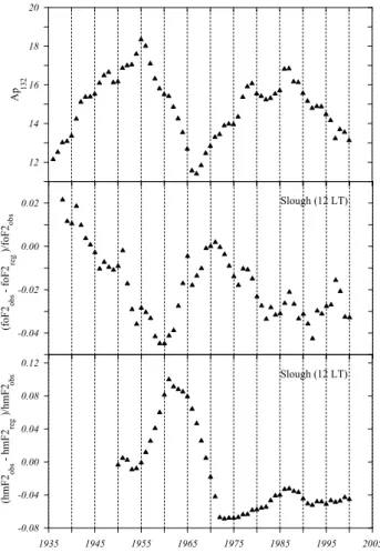
2534 A. V. Mikhailov: Ionospheric long-term trends 14 Figure 1 12 14 16 18 20 Ap . 132 -0.04 -0.02 0.00 0.02 (foF2 foF2 ) /foF2 ob s ob s reg Slough (12 LT) . 1935 1945 1955 1965 1975 1985 1995 2005 -0.08 -0.04 0.00 0.04 0.08 0.12 (h mF2 hmF2 )/ hmF 2 ob s ob s reg Slough (12 LT)
Fig. 1. 11-year running mean Ap index, Ap 132 (top panel),
δfoF2132(middle panel), and δhmF2132(bottom panel) long-term
variations at noon for Slough station.
the last three decades. The thermosphere cooling due to a CO2increase is one of these processes.
The aim of the paper is to analyze both hypotheses by tak-ing into account the available results on the ionosphere and thermosphere parameter long-term variations, and to see if these hypotheses can be reconciled and to what extent they can be reconciled.
2 Trend morphology
In the framework of the geomagnetic control concept the ionospheric trends revealed in foF2, hmF2 and foE depend on geomagnetic activity. Without special efforts to remove these geomagnetic activity effects the ionospheric trends ex-hibit the following morphology (see earlier cited references). 1. The sign (positive/negative) of the trend depends on the phase (increasing/decreasing) of the geomagnetic activ-ity long-term variation, as presented by the Ap132index (11-year running mean Ap). Figure 1 shows the aspect of ge-omagnetic activity variation on δfoF2 and δhmF2 for the Slough station, with the longest available period of
observa-tions. These dependencies until 1995 were given earlier by Mikhailov (2002) and here they are extended until 2000, us-ing recent observations. The 11-year runnus-ing mean δfoF2 and δhmF2 at 12:00 LT are given in comparison with the
Ap132 index variation. Periods of increasing geomagnetic activity (before 1955 and 1968–1986) are seen to correspond to negative trends in foF2 and positive trends in hmF2, with a 4–5 year lag with respect to the Ap132variation. The in-verse situation takes place for the period of decreasing ge-omagnetic activity (1956–1967), with strong positive foF2 and negative hmF2 trends. The anti-phase variations with a 5-year shift between Ap132 and δfoF2132 are seen even in detail, for instance, in the 1980–1990 period.
But this relationship with geomagnetic activity changes for δhmF2132 after 1972. The 1980–1990 peak in Ap132 is a little bit lower than the 1955 one, and δfoF2132 prop-erly reflects this two-hump variation in Ap132. Qualitatively,
δhmF2132 variations also reflect the Ap132 changes but the magnitude of the δhmF2132 peak is incomparable with the 1960–1965 one (Fig. 1, bottom). This is a very interesting result which may be related to the thermosphere cooling (to be discussed later).
The difference in the sign of the trends during increas-ing/decreasing phases of the geomagnetic activity takes place for all local time moments (Mikhailov and Marin, 2000). Therefore, one should be careful with the selection of time periods for trend analysis and not combine years belonging to different (rising/falling) phases of geomagnetic activity. Unfortunately, this is not taken into account in other publi-cations devoted to the F2-layer parameter trends and this (as one of the reasons) results in chaos of various signs and mag-nitudes of the trends at various stations (e.g. Bremer, 1998, 2001; Upadhyay and Mahajan, 1998).
2. The foF2 trend magnitude depends on the geomagnetic (invariant) latitude, while no pronounced latitudinal depen-dence exists for the hmF2 trends. The dependepen-dence of the
foF2 trend magnitude on the geomagnetic latitude was
re-vealed by Danilov and Mikhailov (1998, 1999) and that was the first indication that F2-layer trends might be related to geomagnetic activity. Mikhailov and Marin (2000) consid-ered this dependence for the increasing phase of geomag-netic activity using various year selections and found a de-pendence of foF2 trends on invariant magnetic latitude. The analysis was repeated by Mikhailov (2002), using the exact years corresponding to the periods of increasing (1970-1985) and decreasing (1959–1970) geomagnetic activity. Negative
foF2 trends were confirmed for all 29 stations considered
for the rising phase of geomagnetic activity and 8 available stations gave positive trends for the falling geomagnetic ac-tivity. Moreover, all trends were significant at the 95–99% confidence level with only one exception of Ekaterinburg. The calculated foF2 trends exhibit a pronounced dependence on geomagnetic (invariant) latitude. High-latitude stations demonstrate the largest negative (positive) trends for rising (falling) periods of geomagnetic activity while low-latitude
stations exhibit relatively small trends (Fig. 3 in Mikhailov, 2002).
Longitudinal differences in the foF2 and hmF2 trends were revealed by Bremer (1998) and in hmF2 trends by Marin et al. (2001). The trends were mostly negative in western Eu-rope and positive in the region east of 30–37◦E.
3. There exist strong diurnal variations of the foF2 and
hmF2 trend magnitude, depending on latitude. A detailed
analysis of these variations for the period with rising ge-omagnetic activity may be found in Mikhailov (2002) for the auroral station Sodankyla (8inv=63.59◦), mid-latitude station Moscow (8inv=51.06◦), and lower-latitude station Alma-Ata (8inv=35.74◦). It was shown that the foF2 trends are strongly negative at high and middle latitudes, with a tendency to be small or positive at lower latitudes. The
foF2 trends revealed are significant at the 95–99% confidence
level for most of the LT moments. Trends in hmF2 also ex-hibit large diurnal variations which are consistent with the
foF2 trend pattern in the framework of F2-layer storm
mech-anism. This is an essential aspect of the F2-layer trend analy-ses which is never discussed in other publications. The elec-tron concentration NmF2 and the height of the F2-layer maxi-mum hmF2 are related by the mechanism of the F2-layer for-mation; therefore the two trends should demonstrate a con-sistent pattern which could be explained in the framework of the contemporary F2-layer theory.
4. A geomagnetic control of the long-term trends has been revealed in the E-region, as well (Mikhailov and de la Morena, 2003). By analogy with the F2-layer periods of increasing geomagnetic activity correspond to negative
foE trends while these trends are positive for the
decreas-ing phase of geomagnetic activity. But this “natural” rela-tionship breaks down around 1970 (on some stations later) when pronounced, positive foE trends have appeared at most of the stations considered. But since this positive foE trend is usually related to the worldwide greenhouse effect, in fact, it does not take place at all stations – the sign of the trends may be different. It is better to point out the spotty global pat-tern with unsystematic foE behavior at different stations after 1970. It is only possible to conclude that since the beginning of 1970s there has appeared an additional factor in the lower thermosphere which has broken down the normal foE depen-dence on geomagnetic activity over a long-term time scale.
The whole enumerated trend morphology cannot be ex-plained neither quantitatively nor qualitatively by the green-house hypothesis. We are still very far from the CO2 dou-bling in the Earth’s atmosphere, but the observed trends are already 3–5 times larger than expected from the greenhouse hypothesis (Bremer, 2001). Given this, some authors stress that the changes in the upper atmosphere or the accuracy of the trends found are not sufficient enough to confirm the greenhouse hypothesis (Upadhyay and Mahajan, 1998; Ulich et al., 2000). On the other hand, the results by Keating et al. (2000), Emmert et al. (2004) and Marcos et al. (2005) on
the thermospheric density decrease seem to be the only direct confirmation for this hypothesis.
3 Numerical estimates
A comparison of the foF2 trends obtained by different scien-tists has been undertaken by Laˇstoviˇcka et al. (2006). Day-time (11:00–14:00 LT) monthly median foF2 observations at Juliusruh for the 1976-1996 period were used in that compar-ison. The scatter in trends obtained turned out to be large but it was summed up that the trend was negative with a mag-nitude of 0.01–0.02 MHz/year. An analysis by Emmert et al. (2004) fulfilled over the 1969–2001 period gave a thermo-spheric density ρ decrease of about –3.0±0.4% per decade at the 480–530-km range, while Marcos et al. (2005), for the same 1970–2000 period and around the ≈400-km height, es-timated a decrease = –1.7±0.2% per decade, i.e. about two times less. The difference in the height range is not very important as the thermospheric neutral density above 350– 400 km is practically presented by atomic oxygen [O], espe-cially during low solar activity considered in our estimates.
Let us take for our analysis a 30-year (1965–1995) period which overlaps or in general coincides with the two men-tioned periods. So we may accept that over this period the
foF2 decrease is 0.3–0.6 MHz and the thermospheric density
decrease is 5–10%. Furthermore, both foF2 and NmF2 (foF2
∝NmF20.5) parameters will be used in our analysis. Accept-ing an average daytime foF2=8 MHz, we have a (4–7)% rel-ative decrease in foF2 or (8–14)% in NmF2. A 5–10% crease in ρ may be totally attributed to a corresponding de-crease in [O] at the heights considered.
But just a thermosphere temperature Tn decrease (for in-stance, due to CO2forcing) which could provide a necessary decrease in ρ, does not produce the required NmF2 variations as the [O] decrease in this case is practically compensated by the [N2] decrease while the direct effect of Tn variations is small (Ivanov-Kholodny and Mikhailov, 1986). This is seen from the expression for the mid-latitude daytime F2-layer (Mikhailov et al., 1995)
1lg Nm = 4/31lg[O] − 2/31lg[N2] −5/61lgTn. (1)
This expression is invariant relative to height changes in the isothermal thermosphere, so any height in the F2-region may be chosen as the basic level for estimates.
The same conclusion follows from the isobaric F2-layer concept by Rishbeth and Edwards (1989, 1990). According to this concept the F2-layer peak follows, in its variations, the level of constant atmospheric pressure. This is a good approximation, at least during daytime hours, when vertical plasma drifts are not strong. It can be shown (Mikhailov and Marin, 2000) that the [O]/[N2] ratio remains constant at any fixed value of pressure and at any temperature height profile, provided temperature and concentrations [O] and [N2] are constant at the base level. Therefore, the observed negative
2536 A. V. Mikhailov: Ionospheric long-term trends trend in NmF2 cannot be explained just by the thermosphere
cooling and the [O]/[N2] ratio should be changed by some other way.
Dynamical processes related to neutral gas upwelling and downwelling are known to result in [O]/[N2] ratio changes, and the contemporary F2-layer storm mechanism is based on this idea (e.g. Rishbeth and M¨uller-Wodarg, 1999). The in-creasing geomagnetic activity is accompanied by an [O]/[N2] ratio decrease at high and middle latitudes, due to gas up-welling in the auroral zone, followed by its transfer to mid-dle latitudes. This effect is reflected to some extent in mod-ern empirical thermospheric models, such as NRLMSISE-00 (Picone et al., 2002), but its magnitude is not large enough (to be discussed later).
So the problem may be formulated as follows. Is it possi-ble to reconcile an expected 10–20 K decrease in the thermo-spheric temperature under the greenhouse hypothesis (Rish-beth and Roble, 1992; Akmaev, 2003), a 5–10% decrease in the thermospheric density (Emmert et al., 2004; Marcos et al., 2005, a (8–14)% decrease in NmF2 (Laˇstoviˇcka et al., 2006), and hmF2 long-term variations with a small positive trend after 1972 (Fig. 1, bottom)?
At first let us check what can be obtained with the NRLMSISE-00 empirical model. Annual mean values of F10.7 are close for the two years chosen (76.3 for 1965 and 77.2 for 1995), therefore no special reduction in solar activity is needed, while the 11-year running mean Apvalues are dif-ferent,12.3 and 14.4, for the two years in question (Fig. 1). All calculations were made for middle latitudes 45–55◦N, 15◦E (close to Juliusruh location) at the 400-km height.
According to Keeling et al. (1995), one may expect a
≤15% increase in [CO2] over a 30-year period and the ther-mospheric temperature decrease by 10–20 K at best (Rish-beth and Roble, 1992; Akmaev, 2003). So for our estimates we may accept 1T n = –15 K , and this is ≤2% for the annual mean Tn over the period considered. Due to an Ap index increase, the annual mean temperature increases by 5–7 K (depending on latitude) and under expected 1T n = –15 K we obtain an overall T n decrease by ≈8–10 K. This gives a 5% decrease in N2 and O2 concentrations and a 4% decrease in [O]. Equation (1), in accordance with earlier comments, gives 1NmF2≈0 in this case. It seems that the dynamical ef-fects on O/N2changes due to geomagnetic activity variations should be presented more strongly. Therefore, if we come from a 10% decrease in ρ (Emmert et al., 2004), a 15-K de-crease in T n, and a 10% dede-crease in NmF2, then from Eq. (1) the required decrease in [N2] should be –2.5% while the
NRLMSISE-00 model gives 1[N2] = –7% and 1[O] = –5%,
i.e. the thermosphere should be more impoverished with atomic oxygen and more abundant with molecule species un-der such an increase in geomagnetic activity. In case of a 5% decrease in ρ (Marcos et al., 2005) the model provides the required decrease in [O] while the [N2] decrease again is overestimated by ≈2.5%.
The routinely obtained F2-layer maximum height hmF2, which is usually used in trend analyses, is a much less reli-able (compared to foF2) parameter, as it is not scaled directly from ionograms but is calculated from the M(3000)F2 pa-rameter using empirical expressions. Nevertheless, the hmF2 long-term variations are consistent with the Ap132and foF2 variations pattern (Fig. 1), which is explained in the frame-work of the geomagnetic control concept (Mikhailov, 2002). But since 1972 the situation has changed. Although qual-itatively the δhmF2 variation reflects, as it did earlier, the variations in Ap132, its magnitude is much less compared to the 1955–1965 period (Fig. 1). This may be considered as a direct confirmation of the thermosphere cooling due to the CO2 increase – the effect which scientists are persistently looking for in the ionospheric trends. Unlike NmF2, which is relatively insensitive to neutral temperature changes, hmF2 is directly related to T n, as it is seen from the expression (Ivanov-Kholodny and Mikhailov, 1986)
hm∝ 2.3H 3 ( lg[O]1+lg β1+lg H2 0.54d !) +cW , (2)
where H=kTn/mg is the scale height and [O] is the con-centration of atomic oxygen, β is the linear loss coef-ficient at a fixed height h1, W (in m/s) is the vertical plasma drift velocity, c is a coefficient close to unity, d=1.38∗1019∗(Tn/1000)0.5 is a coefficient in the expression for the ambipolar diffusion coefficient D=d/[O].
According to the earlier estimates, neutral temperature T n, atomic oxygen concentration [O], and linear loss coefficient
β∝[N2]Tn2are decreasing for the period in question. This should result in a negative hmF2 trend, however, it is slightly positive for the period after 1972. The only possible expla-nation is to accept an increase in the vertical plasma drift W due to the thermospheric neutral winds enhancement. This does not look unreasonable, as the enhancement of the equa-torward (or damping the poleward) thermospheric wind due to increasing geomagnetic activity is well established (e.g. Fejer et al., 2000; Emmert et al., 2001).
4 Discussion
It seems that the geomagnetic activity impact on the upper atmosphere has not yet been fully understood and properly taken into account in the empirical thermospheric models. A large 4±1 year delay between long-term geomagnetic activ-ity variations and long-term F2-layer parameter trends shown earlier on 29 stations (Mikhailov, 2002) and also clearly seen at Slough (Fig. 1) tells us that the whole Earth’s atmosphere is involved with the processes provoked by geomagnetic ac-tivity. Changes in the global atmospheric circulation and related variations in the thermospheric neutral composition and temperature is the most probable mechanism. Short-term (3-h, daily, monthly and perhaps even annual) variations of geomagnetic activity presented by corresponding indices
only produce an effect of “ripples on the water surface” while the atmosphere lives its own life. Therefore, all attempts to remove the geomagnetic activity effects from long-term ionospheric trends, using monthly or even annual mean Ap indices, turn out to be inefficient and only insert additional noise to the analyzed data. As it was shown in our approach (Mikhailov et al., 2002), by working with an 11-year run-ning mean and additionally smoothed Ap, δfoF2, and δhmF2 values, it is possible to remove geomagnetic activity effects to a great extent. The residual trends after such a removal of geomagnetic activity are very small and usually statis-tically insignificant. This was confirmed by the results of different methods comparison using Juliusruh observations (Laˇstoviˇcka et al., 2006). Our foF2 residual trend turned out to be much less (–0.00086 MHz/year) compared to other es-timates (–0.01–0.02) MHz/year. But if we did not remove the geomagnetic activity effects from our results, then the trend estimated over the whole 1976-1996 period would be ≤– 0.01 MHz/year (depending on the accepted average foF2=8– 10 MHz), which coincides with the other estimates. It should be noted that the 1976–1996 period comprises both the ris-ing until 1987 and the fallris-ing phases of geomagnetic activ-ity with different trend magnitudes. For instance, if one takes only the 1976–1987 period (rising phase), the trend will be ≈ –0.03 MHz/year, i.e. even higher than other esti-mates. Thus, large (–0.01 –0.02) MHz/year trends obtained by other scientists are just due to geomagnetic activity ef-fects which have not been removed properly from the ana-lyzed data. A small negative residual trend obtained with our approach (Mikhailov et al., 2002) reflects a very long-term increase in the geomagnetic activity which took place in the 20th century.
Coming back to the main question of the paper: if the geomagnetic control and the greenhouse hypotheses can be reconciled, it should be answered – yes. The basic (natu-ral, background) NmF2 and hmF2 long-term variations are controlled by long-term variations of the geomagnetic activ-ity using standard F2-layer storm mechanisms. The thermo-sphere cooling due to the greenhouse effect (other possible effects of CO2 increase are not discussed in relation with the ionospheric trends) is practically not noticeable in the
foF2 trends. This is due to a weak NmF2 dependence on
neutral temperature. Therefore, foF2 trends are completely controlled by long-term variations of the geomagnetic activ-ity, if, of course, its effects are not removed. A two-hump structure in Ap132variations is clearly reproduced in the foF2 long-term variations with a 4–5 year lag (Fig. 1). This rela-tionship is seen even in detail, for instance, in the two peaks and the valley in 1980–1990 as part of the foF2 variations. A similar relationship of long-term trends with the geomag-netic activity takes place in the ionospheric E-region, as well (Mikhilov and de la Morena, 2003), although the mechanism of this relation in the E-region is quite different (Mikhailov, 2006).
A 4–5 year delay in F2-layer trends with respect to Ap132 variations is a very interesting and yet unexplained effect. It was revealed in our earlier trend analyses, where we pro-posed that such a large time delay might imply that the whole Earth’s atmosphere is involved with the processes provoked by geomagnetic activity. Changes in the global atmospheric circulation and related variations in the thermospheric neu-tral composition and temperature is the most probable mech-anism. Obviously, this time lag tells us about the charac-teristic time of the Earth’s atmosphere. According to some model estimates, it takes about 5 years for tropospheric air to reach the mesospheric heights (Schneider et al., 2000) and this estimate seems to confirm the idea.
The situation with the hmF2 trend is more complicated. There are serious problems with using routine hmF2 data for trend analyses (Ulich, 2000) and the priority should be given to foF2 trends, based on direct and more reliable ob-servations, while hmF2 trends may be considered only as complimentary information which should not at least con-tradict the mechanism proposed. However, any hypothesis should explain both NmF2 and hmF2 long-term trends in a consistent way, as these parameters are related by the F2-layer formation mechanism. Until now no reasonable hy-pothesis of the F2-layer parameter trends has been proposed, except for the geomagnetic control concept. The anti-phase
NmF2 and hmF2 long-term variations take place at Slough
(Fig. 1) and such variations are explained in the framework of the F2-layer storm mechanism (Mikhailov, 2002 and ref-erences therein). Unlike NmF2, which is not very sensitive to the neutral temperature and vertical plasma drift (during daytime) variations, hmF2 depends directly on both param-eters (Eq. 2). Therefore, the expected thermosphere cool-ing under the greenhouse hypothesis should be seen in hmF2 variations (see also Rishbeth, 1990). Indeed, the “humps” in Ap132around 1955 and 1987 are close in magnitude and this is adequately reflected in foF2 variations but not in hmF2 variations (Fig. 1). This result may be considered as a direct confirmation for the thermosphere cooling. Although we still have hmF2 variations which follow the geomagnetic activity ones, the amplitude of these changes is strongly depressed.
According to earlier quantitative estimates the only pos-sibility to maintain a positive hmF2 trend after 1972 is to accept an increase in the vertical plasma drift W due to ther-mospheric winds. Obviously, a similar W increase took place during the previous period of elevated geomagnetic activ-ity around 1955, but then it was in line with the increase in thermosphere temperature and linear loss coefficient, in ac-cordance with the F2-layer storm mechanism and this gave a large peak in hmF2 variations (Fig. 1). After 1972 we have small negative trends in all aeronomic parameters (see Eq.( 2)), as a result of competition between the thermosphere cooling (due to a CO2increase) and heating (due to an Ap132 increase). Under such conditions, the contribution of W to hmF2 variations increases, that is the disturbed thermo-spheric winds start to play the leading role.
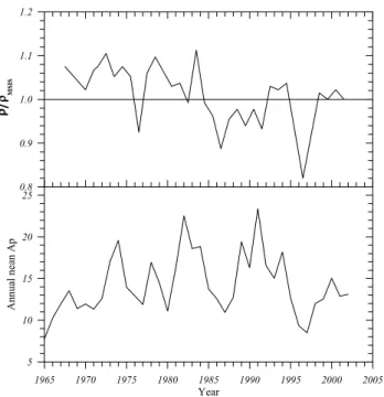
2538 A. V. Mikhailov: Ionospheric long-term trends 15 Figure 2. 1965 1970 1975 1980 1985 1990 1995 2000 2005 Year 5 10 15 20 25 An nua l nea n Ap 0.8 0.9 1.0 1.1 1.2 MS IS
Fig. 2. Annual averages ρ /ρMSI S(from Emmert et al., 2004) and
annual mean Apindices.
The confirmation to these ideas can be found in previous results of the ionospheric trend analyses. Bremer (1998) has revealed negative trends in hmF2 in the European region west of 30◦E while positive trends dominated in the region to the east from 30◦E. A similar conclusion on hmF2 trends has been obtained by Marin et al. (2001), who used quite a differ-ent method for trend analysis. Whereas most of the analyzed stations located in the 0–22◦E longitudinal sector exhibited negative trends, those eastward from 37◦E presented signifi-cant positive trends. Stations located in the transitional (26– 33◦E) region gave small and insignificant positive or nega-tive trends. The analyzed period includes the rising phase of geomagnetic activity after 1965 when the thermosphere cooling effects have become noticeable. This longitudinal separation clearly indicates the geomagnetic field of origin of the effect. The 20◦E longitude in Europe corresponds to a zero declination (D) of the magnetic field, therefore, zonal (westward) wind Vny will produce negative plasma drift in western Europe, where D<0, and positive drift in the east-ern region, where D>0, in accordance with the expression W =–VnySinICosISinD, where I is magnetic inclination pos-itive in the Northern Hemisphere. An enhancement of the disturbance westward thermospheric wind has been reported by Emmert et al. (2001) using WINDII observations. Both zonal and meridional perturbations were found to increase roughly linearly with Kpand expand to lower latitudes with increasing magnetic activity.
Summarizing this part of our analysis it should be stressed that the mechanism of the F2-layer parameter long-term trends is pretty sophisticated and cannot be reduced to one
process (the thermosphere cooling, for instance), but in ac-cordance with the theory of F2-layer formation it includes some different processes, the role and contribution each of them vary with conditions. Without the thermosphere cool-ing due to a CO2increase the NmF2 and hmF2 trend pattern would be determined by long-term variations of geomagnetic activity via the standard F2-layer storm mechanisms. This still takes place for NmF2 but not for hmF2 trends, for which the situation has changed after 1972 when the thermosphere cooling became noticeable and the disturbed (again due to the increasing geomagnetic activity) winds appeared on the stage to play an important role.
In the framework of our analysis we should say some words about the results by Keating et al. (2000), Emmert et al. (2004) and Marcos et al. (2005), as they are closely related to the ionospheric trends mechanism. In the cited pa-pers it is directly stated that the observed density decrease is associated with the cooling effect of increased greenhouse gas concentrations. Yes, a 20 K decrease in T n provides the observed ≈10% decrease in neutral density (Emmert et al., 2004) at 400 km over a 30-year period. A 10-K decrease in
T nis needed for a 5% decrease in ρ in the case of the Marcos et al. (2005) results. But as it was shown earlier just a temper-ature decrease alone does not explain the negative trends in
foF2 obtained over about the same period; the result has been
confirmed by different authors using all available ionosonde observations and should be considered as reliable. To rec-oncile these results we should accept for the period in ques-tion more pronounced O/N2changes (with larger [O] and less [N2] decreases) under the variations of geomagnetic activity than provide empirical thermosphere models, NRLMSISE-00, for instance. The effect is probably related to gas up-welling in the auroral zone, due to the thermosphere heating under increasing geomagnetic activity. Therefore, the ob-served density decrease is due to two processes – the thermo-sphere cooling and the atomic oxygen abundance decrease resulting from the disturbed thermospheric circulation. But such neutral composition changes are not predicted by mod-ern thermospheric empirical models.
The restriction of empirical models in describing disturbed conditions has been stressed repeatedly. For instance, a comparison of thermospheric parameters retrieved from EIS-CAT (auroral zone) observations with MSIS-86 predictions (Mikhailov and Lilensten, 2004) has shown that the model strongly overestimates both total gas density ρ and atomic oxygen concentration at 300 km for disturbed days with an average ρcal/ρMSI S=0.52 and [O]cal/[O]MSI S=0.43. Both differences are significant at the 99% confidence level. A similar result was obtained by Litvin et al. (2000) by ana-lyzing with the energy equation Millstone Hill (middle lati-tudes) incoherent scatter observations for a disturbed period of 5–11 June 1991. During the most active phase of the dis-turbance, they found [O] to be lower by a factor of 2 than MSIS-86 predictions. Negative F2-layer storm effects, which are due to an O/N2 ratio decrease, cannot be satisfactory
modelled without a special fitting of aeronomic parameters for each particular ionospheric storm (e.g. Richards et al., 1989, 1994; Buonsanto, 1999).
The importance of the removal of the effects of geomag-netic activity for adequate analysis of the long-term trends has been stressed in this paper, as well as in our previous publications on the problem. When this is not properly done or when geomagnetic effects are removed only partly, the an-alyzed long-term variations, in fact, present the variations of geomagnetic activity and it is not clear which trends are ana-lyzed. The results by Emmert et al. (2004) are not free from this drawback, as well. Their linear trend –3.1±0.9% per decade (their Fig. 2) was drawn over ρ/ρMSI S values which demonstrate large but systematic variations. Our analysis of their results (Fig. 2) shows that practically all ups and downs in ρ/ρMSI S variations coincide within 1 year with changes (corresponding ups, downs or bends in the curve) in the annual mean Ap index. On the one hand, this tells us that NRLMSISE-00 used in their analysis does not work out properly the long-term variations in solar and geomag-netic activity. On the other hand, this means that long-term geomagnetic activity effects were not removed from the ana-lyzed ρ/ρMSI Svariations. Which long-term trend in the ther-mospheric density will be left after such a removal is an open question.
The results by Marcos et al. (2005), obtained over the same period, give a two times smaller trend in the thermospheric density –1.7 ±0.2% per decade. One of the reasons for this difference may be due to the reduction procedure used in their analysis. A relatively old thermospheric model by Jac-chia (1970) has been chosen for the drag measurements re-duction. Obviously, this choice was not random, as among many others this is the only model which takes into account the running annual mean Kpindex variations. This feature of the model is very important for long-term trend analysis, as it allows one to remove or suppress the geomagnetic activity long-term variation effects. From this point of view a more moderate trend obtained by Marcos et al. (2005) looks more realistic.
5 Conclusions
The main results of our consideration may be summarized as follows.
1. Long-term variations of geomagnetic activity are cru-cial for ionosphere and thermosphere long-term trend anal-yses. Via changes in thermospheric circulation and corre-sponding changes in neutral composition and temperature the geomagnetic activity determines the basic pattern of the ionospheric trends. Additional processes, such as thermo-sphere cooling due to a CO2increase, overlapping the basic pattern may change it to some extent but is unable to explain the observed ionospheric trend morphology. Therefore, be-fore any analysis of long-term trends, basic long-term
varia-tions related to geomagnetic activity should be removed from the analyzed material. This needs special methods and is usu-ally not done by researchers; therefore, the resultant trends turn out to be strongly “contaminated” with the geomagnetic activity effects.
2. Just a thermosphere temperature decrease, which is ac-cepted by many as an explanation for the neutral density de-crease, cannot explain negative foF2 trends revealed for the same period by many ionospheric research studies. The ob-served density decrease comprises of two parts – one is due to direct thermosphere cooling and the other to an atomic oxy-gen abundance decrease, presumably the result of disturbed thermospheric circulation. The quantitative contribution of each process depends on the accepted decrease in the ther-mospheric density. But there are doubts in the magnitude of the neutral density trend given by Emmert et al. (2004), as their results are not free from geomagnetic activity effects.
3. Thermosphere cooling can be reconciled with the
geomagnetic control concept by accepting a more pro-nounced dependence of the O/N2ratio on geomagnetic ac-tivity than is presented by empirical thermospheric models like NRLMSISE-00. This drawback of empirical models on a short-term time scale is well-known and has been stressed repeatedly. The effects of long-term geomagnetic activity variations are not taken into account in such models, in prin-ciple, and this is seen in the Emmert et al. (2004) results.
4. Thermospheric cooling practically cannot be seen in
foF2 trends, due to a weak NmF2 dependence on neutral
tem-perature; therefore, foF2 trends are mainly controlled by geo-magnetic activity long-term variations. This is confirmed by long-term foF2 variations revealed for the whole 1938–2000 period at the Slough station. Large (–0.01–0.02) MHz/year trends obtained by a majority of researchers (Laˇstoviˇcka et al., 2006) just reflect the unremoved effects of geomagnetic activity for the period in question. Such trends would be pos-itive if the 1960–1970 period was considered. Real residual
foF2 trends, which are free to a great extent of geomagnetic
activity effects, are very small and usually statistically in-significant.
5. Long-term hmF2 variations are also controlled by ge-omagnetic activity variations, as both parameters NmF2 and
hmF2 are related by the F2-layer formation mechanism. But
unlike NmF2 the F2-layer maximum height is very sensi-tive to neutral temperature and thermospheric wind varia-tions. Strongly damped hmF2 long-term variations observed at Slough after 1972 are a direct manifestation of the thermo-sphere cooling. A competition between thermothermo-sphere heat-ing (due to the increasheat-ing geomagnetic activity) and its cool-ing (due to CO2increase) gave an opportunity for thermo-spheric winds to appear themselves. Revealed earlier by Bre-mer (1998) and Marin et al. (2001) negative hmF2 trends in Western Europe (where magnetic declination D<0) and posi-tive trends in the eastern stations (where D>0) can be related to enhanced westward thermospheric wind.
2540 A. V. Mikhailov: Ionospheric long-term trends
Acknowledgements. Topical Editor M. Pinnock thanks two referees
for their help in evaluating this paper.
References
Akmaev, R. A.: Thermospheric resistance to “greenhouse cooling”: Effect of the collisional excitation rate by atomic oxygen on the thermal response to CO2forcing, J. Geophys. Res., 108, 1292,
doi:10.1029/2003JA009896, 2003.
Bremer, J.: Ionospheric trends in mid-latitudes as a possible indica-tor of the atmospheric greenhouse effect, J. Atmos. Terr. Phys., 54, 1505–1511, 1992.
Bremer, J.: Trends in the ionospheric E and F regions over Europe, Ann. Geophys., 16, 986–996, 1998,
http://www.ann-geophys.net/16/986/1998/.
Bremer, J.: Trends in the thermosphere derived from global ionosonde observations, Adv. Space Res., 28, (7)997–(7)1006, 2001.
Buonsanto, M. J.: Ionospheric storms – a review, Space Sci. Rev., 88, 563–601, 1999.
Danilov, A. D. and Mikhailov, A. V.: Long-term trends of the F2– layer critical frequencies: a new Approach, Proceedings of the 2nd COST 251 Workshop “Algorithms and models for COST 251 Final Product”, 30–31 March, 1998, Side, Turkey, Ruther-ford Appleton Lab., UK, 114–121, 1998.
Danilov, A. D. and Mikhailov, A. V.: Spatial and seasonal variations of the foF2 long-term trends, Ann. Geophys., 17, 1239–1243, 1999,
http://www.ann-geophys.net/17/1239/1999/.
Danilov, A. D. and Mikhailov, A. V.: F2-layer parameters long-term trends at the Argentine Islands and Port Stanley stations, Ann. Geophys., 19, 341–349, 2001,
http://www.ann-geophys.net/19/341/2001/.
Emmert, J. T., Fejer, B. G., Fesen, C. G., Shepherd, G. G., and Sol-heim, B. H.: Climatology of middle- and low-latitude daytime F region disturbance neutral winds measured by Wind Imaging Interferometer (WINDII), J. Geophys. Res., 106, 24 701–24 712, 2001.
Emmert, J. T., Picone, J. M., and Lean, J. L.: Global change in the thermosphere: Compelling evidence of a sec-ular decrease in density, J. Geophys. Res., 109, A02301, doi:10.1029/2003JA0101176, 2004.
Fejer, B. G. and Emmert, J. T.: Average daytime F region distur-bance neutral winds measured by UARS: Initial results, Geo-phys. Res. Lett., 27, 1859–1862, 2000.
Givishvili, G. V. and Leshchenko, L. N.: Possible proofs of pres-ence of technogenic impact on the mid-latitude ionosphere (in Russian), Doklady RAN, 334, (1), 213–214, 1994 .
Jacchia, L. G.: New static models of the thermosphere and exo-sphere with empirical temperature profiles, Spec. Rep. Smithon. Astrophys. Obs., No 313, 87, 1970.
Jarvis, M. J., Jenkins, B., and Rodgers, G. A.: Southern hemisphere observations of a long-term decrease in F region altitude and thermospheric wind providing possible evidence for global ther-mospheric cooling, J. Geophys. Res., 103, 20 774–20 787, 1998. Ivanov-Kholodny, G. S. and Mikhailov, A. V.: The prediction of
ionospheric conditions, Reidel, Dordrecht, 168, 1986.
Keating, G. M., Tolson, R. H., and Bradford, M. S.: Evidence of long term global decline in the Earth’s thermospheric density
ap-parently related to anthropogenic effects, Geophys. Res. Lett., 27, 1523–1526, 2000.
Keeling, C. D., Whorf, T. P., Wahlen, M., and van der Pflicht, J.: Interannual extremes in the rate of rise of atmospheric carbon dioxide since 1980, Nature, 375, 666–670, 1995.
Laˇstovi`eka, J., Mikhailov, A. V., Ulich, T., Bremer, J., Elias, A. G., Ortiz de Adler, N., Jara, V., Abarca del Rio, R., Foppiano, A. J., Ovalle, E., and Danilov, A. D.: Long-term trends in foF2: a comparison of various methods (in press), J. Atmos. Solar-Terr. Phys., 2006.
Marcos, F. A., Wise, J. O., Kendra, M. J., Grossbard, N. J., and Bowman, B. R.: Detection of long-term decrease in ther-mospheric neutral density, Geoph. Res. Lett., 32, L04103, doi:10.1029/2004GL021269, 2005.
Litvin, A., Oliver, W. L., Picone, J. M., and Buonsanto, M. J.: The upper atmosphere during June 5–11, 1991, J. Geophys. Res., 105, 12 789–12 796, 2000.
Marin, D., Mikhailov, A. V., de la Morena, B. A., and Herraiz, M.: Long-term hmF2 trends in the Eurasian longitudinal sector on the ground-based ionosonde observations, 2001, Ann. Geophys., 19, 761–772, 2001,
http://www.ann-geophys.net/19/761/2001/.
Mikhailov, A. V., Skoblin, M. G., and F¨orster, M.: Day-time F2-layer positive storm effect at middle and lower latitudes, Ann. Geophys., 13, 532–540, 1995,
http://www.ann-geophys.net/13/532/1995/.
Mikhailov, A. V.: The geomagnetic control concept of the F2-layer parameter long-term trends, Phys. Chem. Earth, 27, 595–606, 2002.
Mikhailov, A. V.: Trends in the ionospheric E-region, Phys. Chem. Earth, 31, 22–23, 2006.
Mikhailov, A. V. and Marin, D.: Geomagnetic control of the foF2 long-term trends, Ann. Geophys., 18, 653–665, 2002,
http://www.ann-geophys.net/18/653/2002/.
Mikhailov, A. V. and Marin, D.: An interpretation of the foF2 and
hmF2 long-term trends in the framework of the geomagnetic
con-trol concept, Ann. Geophys., 19, 733–748, 2001, http://www.ann-geophys.net/19/733/2001/.
Mikhailov, A. V., Marin, D., Leschinskaya, T. Yu., and Herraiz, M.: A revised approach to the foF2 long-term trends analysis, Ann. Geophys., 20, 1663–1675, 2002,
http://www.ann-geophys.net/20/1663/2002/.
Mikhailov, A. V. and de la Morena, B. A.: Long-term trends of foE and geomagnetic activity variations, Ann. Geophys., 21, 751– 760, 2003,
http://www.ann-geophys.net/21/751/2003/.
Mikhailov, A. V. and Lilensten, J.: A revised method to extract ther-mospheric parameters from incoherent scatter observations, Ann. Geophysics, Supp., 47, 985–1008, 2004.
Picone, J. M., Hedin, A. E., and Drob, D. P., and Aikin, A. C.: NRLMSISE-00 empirical model of the atmosphere: Statistical comparison and scientific issues, J. Geophys. Res., 107, 1468, doi:10.1029/2002JA009430, 2002.
Richards, P. G., Torr, D. G., Buonsanto, M. J., and Miller, K. L.: The behaviour of the electron density and temperature at Mill-stone Hill during the equinox transition study September 1984, J. Geophys. Res., 94, 16 969–16 975, 1989.
Richards, P. G., Torr, D. G., Buonsanto, M. J., and Sipler, D. P.: Ionospheric effects of the March 1990 magnetic storm:
ison of theory and measurement, J. Geophys. Res., 99, 23 359– 23 365, 1994.
Rishbeth, H.: A greenhouse effect in the ionosphere?, Planet. Space Sci., 38, 945–948, 1990.
Rishbeth, H. and Edwards, R.: The isobaric F2 layer, J. Atmos. Terr. Phys., 51, 321–338, 1989.
Rishbeth, H. and Edwards, R.: Modeling the F2 layer peak height in terms of atmospheric pressure, Radio Sci., 25, 757–769, 1990. Rishbeth, H. and Roble, R. G.: Cooling of the upper atmosphere by enhanced greenhouse gases – Modelling of thermospheric and ionospheric effects, Planet. Space Sci., 40, 1011–1026, 1992. Rishbeth, H. and M¨uller-Wodarg, I. C. F.: Vertical circulation
and thermospheric composition: a modelling study, Ann. Geo-phys.,17, 794–805, 1999.
Roble, R. G. and Dickinson, R. E.: How will changes in carbon dioxide and methane modify the mean structure of the meso-sphere and thermomeso-sphere ?, Geophys. Res. Lett., 16, 1441–1444, 1989.
Schneider, H. R., Jones, D. B. A., Wofsy, S. C., and McElroy, M. B.: Analysis of residual mean transport in the stratosphere; 2. Dis-tributions of CO2and mean age, J. Geophys. Res., 105, 20 013– 20 024, 2000.
Ulich, T. and Turunen, E.: Evidence for long-term cooling of the upper atmosphere in ionospheric data, Geophys. Res. Lett., 24, 1103–1106, 1997.
Ulich, Th., Turunen, E., and Karinen, A.: Global change and chang-ing upper atmosphere-Observations, in: Solar variability and long-term trends in the ionosphere, Sodankyla Geophysical ob-servatory publications, No. 87, 1–14, 2000.
Upadhyay, H. O. and Mahajan, K. K.: Atmospheric greenhouse ef-fect and ionospheric trends, Geophys. Res. Lett., 25, 3375–3378, 1998.