A new atmospheric aerosol phase equilibrium model (UHAERO): organic systems

(1)

HAL Id: hal-00296332

https://hal.archives-ouvertes.fr/hal-00296332

Submitted on 14 Sep 2007

HAL is a multi-disciplinary open access

archive for the deposit and dissemination of

sci-entific research documents, whether they are

pub-lished or not. The documents may come from

teaching and research institutions in France or

abroad, or from public or private research centers.

L’archive ouverte pluridisciplinaire HAL, est

destinée au dépôt et à la diffusion de documents

scientifiques de niveau recherche, publiés ou non,

émanant des établissements d’enseignement et de

recherche français ou étrangers, des laboratoires

publics ou privés.

(UHAERO): organic systems

N. R. Amundson, A. Caboussat, J. W. He, A. V. Martynenko, C. Landry, C.

Tong, J. H. Seinfeld

To cite this version:

N. R. Amundson, A. Caboussat, J. W. He, A. V. Martynenko, C. Landry, et al.. A new atmospheric

aerosol phase equilibrium model (UHAERO): organic systems. Atmospheric Chemistry and Physics,

European Geosciences Union, 2007, 7 (17), pp.4675-4698. �hal-00296332�

(2)

Chemistry

and Physics

A new atmospheric aerosol phase equilibrium model (UHAERO):

organic systems

N. R. Amundson1, A. Caboussat1, J. W. He1, A. V. Martynenko1, C. Landry2, C. Tong3, and J. H. Seinfeld3

1_{Department of Mathematics, University of Houston, Houston, USA}

2_{Chaire d’Analyse et Simulation Numériques, Ecole Polytechnique Fédérale de Lausanne, Lausanne, Switzerland}

3_{Departments of Chemical Engineering and Environmental Science and Engineering, California Institute of Technology,}

Pasadena, USA

Received: 23 May 2007 – Published in Atmos. Chem. Phys. Discuss.: 11 June 2007 Revised: 30 August 2007 – Accepted: 10 September 2007 – Published: 14 September 2007

Abstract. In atmospheric aerosols, water and volatile

inor-ganic and orinor-ganic species are distributed between the gas and aerosol phases in accordance with thermodynamic equilib-rium. Within an atmospheric particle, liquid and solid phases can exist at equilibrium. Models exist for computation of phase equilibria for inorganic/water mixtures typical of at-mospheric aerosols; when organic species are present, the phase equilibrium problem is complicated by organic/water interactions as well as the potentially large number of organic species. We present here an extension of the UHAERO inganic thermodynamic model (Amundson et al., 2006c) to or-ganic/water systems. Phase diagrams for a number of model organic/water systems characteristic of both primary and sec-ondary organic aerosols are computed. Also calculated are inorganic/organic/water phase diagrams that show the effect of organics on inorganic deliquescence behavior. The effect of the choice of activity coefficient model for organics on the computed phase equilibria is explored.

1 Introduction

Atmospheric particles are generally a mixture of inorganic and organic components and water. Water and other volatile species are distributed between the gas and aerosol phases in accordance with thermodynamic equilibrium, and the quan-tities of these species in the aerosol phase at given condi-tions of temperature and relative humidity are determined by the conditions of that equilibrium. A great deal of work has been carried out on the development of thermodynamic models of atmospheric aerosols, as such models are an essen-tial component of more comprehensive atmospheric chemi-cal transport models that treat aerosols. A recent summary of a number of existing thermodynamic models for

inor-Correspondence to: J. H. Seinfeld

(seinfeld@caltech.edu)

ganic aerosols is given by Amundson et al. (2006c). Ther-modynamic models of aerosols containing organic material have also received considerable attention (Saxena and Hilde-mann, 1997; Ansari and Pandis, 2000; Clegg et al., 2001, 2003; Pankow et al., 2001; Seinfeld et al., 2001; Ming and Russell, 2002; Topping et al., 2005; Clegg and Sein-feld, 2006a,b; Metzger et al., 2006; Amundson et al., 2007). Aerosol thermodynamic models that are imbedded within at-mospheric chemical transport models predict, at any time, the gas-particle distribution of volatile species. In the case of inorganic particles, the equilibrium calculation determines whether the aerosol phase is liquid, solid, or a mixture of solid and aqueous phases. When organics are present as well, current models that include both inorganics and organics as-sume a priori either that particles consist of a single-phase inorganic-organic-water mixture or that each particle con-sists of an aqueous phase that contains largely inorganics and water and an organic phase (e.g. Griffin et al., 2002, 2003, 2005). Whereas predicting the phase state of the mixture is a cornerstone of inorganic aerosol models, organic aerosol models do not yet generally have this capability. Predict-ing the phase state of atmospheric organic-containPredict-ing par-ticles is important for a variety of reasons. For example, the presence of organic species in solution may substantially influence the phase transitions that occur when salts deli-quesce and effloresce; likewise, dissolved electrolytes can have appreciable effects on the solubility of organic com-ponents in solution. A new inorganic atmospheric aerosol phase equilibrium model, termed UHAERO, was introduced by Amundson et al. (2006c). In the present work UHAERO is extended for determining the phase equilibrium of organic-water systems. The next section is devoted to a brief sum-mary of the mathematical approach to solving the equi-librium problem, the details of which are given elsewhere (Amundson et al., 2005b, 2006b). Section 3 discusses gen-eral characteristics of organic phase equilibria, and presents a number of examples of organic phase equilibria calculated

(3)

with the model. In Sect. 4 we calculate the effect of or-ganic phase equilibria on inoror-ganic deliquescence behav-ior. Finally, in Sect. 5 we evaluate the sensitivity of the predicted phase diagram in one system (1-hexacosanol/pinic acid/water) to the activity coefficient model used.

2 Modeling approach

The liquid phase equilibrium problem (PEP) for a system

of ns substances in π phases at a specified temperature T

and pressure P and for a given total substance abundance in units of moles is the solution of the constrained minimization problem: min G(y1, . . . , yπ; x1, . . . , xπ)= π X α=1 yαg(xα) (1) subject to xα>0, yα ≥0, α=1, 2, . . . , π, π X α=1 yαxα=b, (2)

where yα is the total number of moles in phase α, xα is the

mole fraction vector (of dimension ns) for phase α, g(xα)

is the molar Gibbs free energy for phase α, and b is the ns

-dimensional vector of the total substance abundances. Con-dition (2) expresses the fact that in calculating the partition of

species j , for j =1, . . . , ns, among π phases, the total

quan-tity of species j is conserved and equals the feed bj.

Re-lation (1) characterizes the phase equilibrium as the global minimum of the total Gibbs free energy, G, of the system.

The molar Gibbs free energy (GFE) g is the relevant ther-modynamic function for the PEP, and is usually defined for

the mole fraction vector x by g(x)=xTµ(x), with xTµ(x)

denoting the scalar product of the two vectors x and µ(x). The chemical potential vector µ(x) is given by

µ(x)=µ0+RT ln a(x),

where R is the universal gas constant, µ0 is the standard

chemical potential vector of liquid species, and a(x) is the activity vector at the mole fraction vector x. On a mole frac-tion scale, the activity of component j , for j =1, . . . , ns, is

expressed as aj=fjxj, where fj is the mole fraction-based

activity coefficient, and xj is the mole fraction of species j .

The PEP as stated in (1) can be reformulated in a normalized form: min Gn(y1, . . . , yπ; x1, . . . , xπ)= π X α=1 yαgn(xα) (3)

subject to condition (2). In (3), the normalized

mo-lar GFE gn is defined for the mole fraction vector x

by gn(x)=xT ln a(x) and is related to the molar GFE g

by gn(x)=(g(x)−xTµ0)/RT . We also have the relation

Gn=(G−bTµ0)/RT for the normalized total GFE of the

system. The fact that the normalization relates G to Gn, via

first a shift by the constant bTµ0then a scaling by the

con-stant RT , implies that the two formulations (1) and (3) of the

PEP are equivalent; that is, if {yα, xα}α=1,π is the solution

of (1) for the feed vector b, it is also the solution of (3) for the same feed vector b, and the converse is also true. In the formulation of the PEP, we assume that all the phases in the system belong to the same phase class so that the molar GFE,

g or gn, is the same for all phases; we assume also that all

substances can partition into all phases and that no reactions occur between the different substances. We are interested in determining the state of the system at the thermodynamic equilibrium, i.e. the number of phases π and their composi-tions {yα, xα}α=1,π.

The detailed description of the numerical solution of the PEP by a primal-dual interior-point algorithm is given by Amundson et al. (2005b, 2006b). Essentially, the numeri-cal minimization technique relies on a geometrinumeri-cal concept of phase simplex of the convex hull of the normalized GFE

gn to characterize an equilibrium solution that corresponds

to a global minimum of the total GFE Gn. The algorithm is

started from an initial solution involving all possible phases in the system, and applies, at each iteration step, a New-ton method to the Karush-Kuhn-Tucker optimality system of (3), perturbed by a log-barrier penalty term, to find the next primal-dual approximation of the solution of (3). A second-order phase stability criterion is incorporated to ensure that the algorithm converges (quadratically) to a stable equilib-rium rather than to any other first-order optimality point such as a maximum, a saddle point, or an unstable local minimum. The key parameters in the phase equilibrium

calcula-tion are the mole fraccalcula-tion-based activity coefficients fj,

j =1, . . . , ns, as functions of the mole fraction vector x.

At-mospheric aerosols comprise a wide range of organic species of diverse chemical structures. The approach that has gen-erally been adopted in thermodynamic modeling of organic aerosol mixtures is to represent the mixture in terms of the or-ganic functional groups present. UNIFAC (UNIQUAC Func-tional Group Activity Coefficients), a semi-empirical ther-modynamic model applying the group contribution concept in which the mixture consists not of molecules but of func-tional groups, is a well-established method for estimating

ac-tivity coefficients fj of organic mixtures (Fredenslund et al.,

1977; Sandler, 1999). The availability of an extensive set of UNIFAC group-interaction parameters permits the charac-terization of complex mixtures of virtually all organic com-pounds of atmospheric interest (Gmehling, 1999; Wittig et al., 2003).

What is ultimately needed in a 3-D atmospheric model is a thermodynamic model that computes both the gas-aerosol partitioning and the aerosol phase equilibrium, whose math-ematical formulation is given as

(4)

=nT_gµg+nTsµs+ π X α=1 yαg(xα), (4) subject to ng>0, nl>0, ns≥0 , xα>0, yα ≥0, α=1, 2, . . . , π , Agng+Alnl+Asns=b , (5) π X α=1 yαxα=nl, (6)

where ng, nl, ns are the concentration vectors in gas, liquid,

and solid phases, respectively, µgand µsare the

correspond-ing chemical potential vectors for gas and solid species, Ag,

Al, As are the component-based formula matrices, and b is

the component-based feed vector. Condition (5) expresses the fact, for example, that in calculating the partition of any chemical component (electrolytes and/or organic species) among gas, liquid and solid phases the total concentration is conserved, while maintaining a charge balance in solution. Condition (6) is similar to condition (2) stating that in cal-culating the partition of liquid species j , for j =1, . . . , ns,

among π phases, the total quantity of species j is conserved

and equals the total abundance nl,j of liquid species j . The

chemical potential vectors for gas and solid species are given by

µg=µ0g+RT ln ag,

µs=µ0s,

where µ0_gand µ0_s are the standard chemical potentials of gas

and solid species, respectively, and agis the activity vector

of the gas species.

Again, the key issue in the phase and chemical equilib-rium calculation of (4) is the estimation of the activity

co-efficients fi as a function of the mole fraction vector x

for a liquid phase. If both electrolytes and organic species are present, the general thermodynamic model used in the present application is based on a hybrid approach, namely, the so-called CSB model (Clegg et al., 2001; Clegg and Sein-feld, 2006a,b), where the activity coefficients for the elec-trolytes and the non-electrolyte organics are computed in-dependently, with the Pitzer, Simonson, Clegg (PSC) mole fraction-based model (Clegg and Pitzer, 1992; Clegg et al., 1992) for water/electrolytes mixtures and UNIFAC models for water/non-electrolyte organic mixtures, respectively.

The CSB model is necessarily based upon the assump-tion of a single solvent (water) in which ions and

or-ganic molecules are dissolved. Additional terms for

electrolyte/non-electrolyte organic contributions to the activ-ity coefficients are consequently expressed on a molalactiv-ity ba-sis from the model of Pitzer. The CSB modeling approach is not intended to be applied to mixed solvent systems con-taining both electrolytes and organic species such as those considered in Sect. 4. Such liquids may have an organic

phase present at equilibrium that contains very little water, and the Pitzer model for electrolyte/non-electrolyte organic contributions to the activity coefficients would be unlikely to be accurate over the full range of compositions and con-centrations. There are many other uncertainties affecting the interactions between electrolytes and non-electrolyte organ-ics, largely caused by a lack of data, which affect both liq-uid/liquid and liquid/solid equilibrium (Clegg et al., 2001). Consequently the terms in the Pitzer model for interactions between electrolytes and non-electrolyte organics are not in-cluded in the thermodynamic equilibrium calculations psented in this paper. Raatikainen and Laaksonen (2005) re-viewed a number of other water/organic/electrolyte activ-ity coefficient models and identified a lack of experimental thermodynamic data as a major constraint to the develop-ment of accurate models. The effect of interactions between electrolytes and non-electrolyte organics on the liquid phase equilibria and on the inorganic deliquescence properties of inorganic/organic/water mixtures will be a subject of future studies.

In Amundson et al. (2006c), a new inorganic atmospheric aerosol phase equilibrium model, termed UHAERO, was in-troduced that is based on a computationally efficient mini-mization of the GFE, G, defined as in (4), but for pure

in-organic gas-aerosol equilibrium, which is a computationally

simpler problem where the number of liquid phases is lim-ited to one, i.e. π =1, and the activity coefficients of aque-ous inorganic electrolyte solutions are predicted by the PSC model. The special algebraic structure of the pure inorganic gas-aerosol equilibrium problem was taken advantage of in the numerical minimization technique of UHAERO that is based on a primal-dual active-set algorithm Amundson et al. (2005a, 2006a). In Amundson et al. (2007), UHAERO is extended to include water-soluble organic compounds to account for the influence of organic solutes in electrolyte mixtures, with application to dicarboxylic acids: oxalic, mal-onic, succinic, glutaric, maleic, malic, and methyl succinic acids. Activity coefficients in inorganic/organic/water mix-tures are predicted via the hybrid CSB model that com-bines the PSC model for inorganic multicomponent solu-tions and the UNIFAC model for water/organic mixtures. We note that, compared to pure inorganic gas-aerosol equi-librium, the addition of water soluble organic compounds neither changes the number of liquid phases in equilibrium, i.e. π remains as 1 and the aqueous phase is the only liquid phase at equilibrium, nor alters the special algebraic structure characterizing the underlying phase equilibrium. Therefore, the same numerical minimization technique of UHAERO, namely, the primal-dual active-set algorithm as presented in Amundson et al. (2005a, 2006a), is employed again in Amundson et al. (2007) for mixed inorganic/(water soluble) organic gas-aerosol equilibrium calculations. As an exam-ple, with the inclusion of one dicarboxylic acid, denoted by

H2R, to the sulfate/ammonium/water system, the additional

(5)

Table 1. Organic compounds considered and their UNIFAC groups. Species # Compound name Carbon number Structure UNIFAC

X1 2-hydroxy-glutaric acid (C5) chain 2 CH2, 1 CH, 1 OH, 2 COOH

X2 adipic acid (C6) chain 4 CH2, 2 COOH

X3 glutaraldehyde (C5) chain 3 CH2, 2 CHO

X4 palmitic acid (C16) chain 1 CH3, 14 CH2, 1 COOH

X5 1-hexacosanol (C26) chain 1 CH3, 25 CH2, 1 OH

X6 nonacosane (C29) chain 2 CH3, 27 CH2

X7 pinic acid (C9) complex 2 CH3, 2 CH2, 2 CH, 1 C, 2 COOH

X8 pinonic acid (C10) complex 2 CH3, 2 CH2, 2 CH, 1 C, 1 CH3CO, 1 COOH

Table 2. UNIFAC energy interaction parameters between the main groups used in this work: UNIFAC/UNIFAC-Peng/UNIFAC-LL.

CH2 OH H2O CO CHO COOH

CH2 × 986.5/986.5/644.6 1318./1318./1300. 476.4/476.4/472.6 677.0/677.0/158.1 663.5/663.5/139.4

OH 156.4/156.4/328.2 × 353.5/265.97/28.73 same same 199.0/224.4/–104.0

H₂O 300.0/300.0/342.4 –229.1/–467.4/–122.4 × –195.4/–195.4/–171.8 –116.0/–116.0/–349.9 –14.09/–69.29/–465.7

CO 26.76/26.76/66.56 same 472.5/472.5/634.8 × same 669.4/669.4/1247.

CHO 505.7/505.7/146.1 same 480.8/480.8/623.7 same × 497.5/497.5/0.750

COOH 315.3/315.3/1744. –151.0/–103.0/118.4 –66.17/–145.9/652.3 –297.8/–297.8/–101.3 –165.5/–165.5/1051. ×

(aqueous), R2− (aqueous), H2R (solid), (NH4)2R (solid),

are treated computationally in the same way as inorganic species. In the present work, UHAERO is further extended to include organic compounds that may not be water solu-ble. Therefore, in equilibrium, multiple liquid phases are al-lowed to form, i.e. π >1, and their equilibrium compositions

{yα, xα}α=1,π are to be determined. Again, the CSB hybrid

approach is employed for the activity coefficient calculation of inorganic/organic/water mixtures. In addition, the under-lying numerical minimization technique of UHAERO in the present work is a hybrid one that combines the primal-dual active-set algorithm for the gas-aerosol (i.e. electrolyte so-lution and solids) equilibrium with the primal-dual interior-point algorithm for the liquid phase equilibrium. Therefore, the overall computational efficiency of the hybrid solution method is dictated by the efficiency of two underlying nu-merical minimization techniques.

3 Characteristics of organic phase equilibria

The method for determining organic/water phase equilib-ria developed here treats, in general, any number of organic compounds. The organic fraction of atmospheric aerosols comprises a complex mixture of compounds from direct emissions and atmospheric gas-to-particle conversion. Even if all compounds were known, inclusion of all in an atmo-spheric model is infeasible. Consequently, one approach is to

represent the complex mixture by a set of model compounds that span the range of properties characteristic of the actual ambient mixture (see, for example, Pun et al., 2002). The set of surrogate compounds should include ones that display characteristics of primary and secondary organics. Primary organics tend to be longer chain aliphatic (and aromatic) species, whereas oxidized secondary species are character-ized by the presence of –OH, –COOH, and –CHO groups. Those chosen for detailed study here are given in Table 1. Palmitic acid (X4), 1-hexacosonol (X5), and nonacosane (X6) are characteristic of primary organic aerosol material, whereas 2-hydroxy-glutaric acid (X1), adipic acid (X2), glu-taraldehyde (X3), pinic acid (X7), and pinonic acid (X8) rep-resent secondary species. Adipic acid and pinic acid/pinonic acid are products of the atmospheric oxidation of cyclohex-ene and alpha-pincyclohex-ene, respectively.

Table 2 shows the three different sets of UNIFAC ters used in this study. Sets of UNIFAC interaction parame-ters were derived from vapor-liquid (Hansen et al., 1991) and liquid-liquid equilibrium data (Magnussen et al., 1981). The most widely used set of parameters derived from vapor-liquid data is referred to as UNIFAC, while those from liquid-liquid equilibrium data are denoted by LL. UNIFAC-Peng parameters are mostly consistent with UNIFAC pa-rameters, except Peng et al. (2001) modified the functional

group interaction parameters of the COOH/H2O, OH/H2O,

and OH/COOH pairs by fitting the UNIFAC model to mea-sured data.

(6)

Table 3. Two-phase equilibrium solutions for binary systems.

UNIFAC UNIFAC-Peng UNIFAC-LL

system (s1/s2) [x(1)s2, xs(2)2] (a(12)s1 , a(12)s2 ) [xs(1)2, x(2)s2] (as(12)1 , as(12)2 ) [xs(1)2, xs(2)2] (a(12)s1 , a(12)s2 )

water/X1 none none none none none none

water/X2 none none none none none none

water/X3 [9.365e-02, 3.453e-01] (9.603e-01, 7.754e-01) [9.365e-02, 3.453e-01] (9.603e-01, 7.754e-01) [4.895e-02, 2.834e-01] (9.741e-01, 5.742e-01) water/X4 [1.188e-07, 8.433e-01] (1-3.22e-07, 8.552e-01) [2.129e-07, 7.585e-01] (1-4.06e-07, 7.671e-01) [2.547e-08, 9.830e-01] (1-2.88e-07, 9.848e-01) water/X5 [2.061e-12, 8.984e-01] (1-2.12e-07, 9.093e-01) [4.020e-12, 7.246e-01] (1-1.80e-06, 5.996e-01) [2.711e-13, 9.142e-01] (1-2.05e-07, 9.196e-01) water/X6 [8.633e-16, 9.976e-01] (1-8.50e-08, 9.977e-01) [8.633e-16, 9.976e-01] (1-8.50e-08, 9.977e-01) [1.000e-16, 9.976e-01] (1-2.69e-07, 9.976e-01) water/X7 [3.351e-03, 3.655e-01] (9.970e-01, 3.980e-01) [8.575e-03, 2.076e-01] (9.935e-01, 1.910e-01) [4.147e-03, 3.508e-01] (9.964e-01, 4.407e-01) water/X8 [1.049e-03, 4.922e-01] (9.990e-01, 5.329e-01) [1.561e-03, 3.894e-01] (9.985e-01, 3.797e-01) [1.078e-03, 4.977e-01] (9.990e-01, 6.036e-01)

X1/X2 none none none none none none

X1/X3 none none none none [5.832e-01,

8.398e-01] (6.896e-01, 9.376e-01) X1/X4 [2.893e-03, 9.808e-01] (9.972e-01, 9.821e-01) [2.885e-03, 9.809e-01] (9.972e-01, 9.823e-01) [1.546e-03, 9.592e-01] (9.985e-01, 9.628e-01) X1/X5 [2.724e-05, 9.797e-01] (1-2.73e-05, 9.800e-01) [2.453e-05, 9.846e-01] (1-2.47e-05, 9.850e-01) [3.744e-05, 9.198e-01] (1-3.75e-05, 9.250e-01) X1/X6 [1.853e-07, 1-8.29e-05] (1-3.52e-07, 1-9.25e-05) [1.934e-07, 1-9.96e-05] (1-3.61e-07, 1-9.87e-05) [4.582e-07, 9.894e-01] (1-6.22e-07, 9.8960e-01)

X1/X[7,8] none none none none none none

Tables 3 and 4 present the complete set of binary and ternary mixtures, respectively, studied here. For each mix-ture the characteristics of the phase equilibrium are summa-rized for each of the three different activity coefficient mod-els, UNIFAC, UNIFAC-Peng, and UNIFAC-LL. In the col-umn of Table 3 corresponding to each of the activity coeffi-cient models, the set {xs(1)2 , x

(2)

s2 }represents the mole fractions

of component 2 at which the two equilibrium phases are lo-cated, xs(1)2 and x

(2)

s2 , and the corresponding equilibrium

activ-ities for each component, as(12)1 and a

(12)

s2 . The entry “none”

in Table 3 indicates that no two-phase equilibrium is pre-dicted for the system. For binary systems, both UNIFAC and UNIFAC-Peng parameters predict similar results, as the two sets of parameters are largely identical. On the other hand, the UNIFAC-LL parameters predict different phase solutions for X1/X3, X2/X(4,5). X3/X(4–6), X5/X(7,8), and X6/X7. As shown in Table 2, the UNIFAC-LL parameters are signif-icantly different from those of UNIFAC and UNIFAC-Peng, leading to the differences in the predictions. We address this issue subsequently

The three-phase equilibrium solutions are presented in Ta-ble 4 for all possiTa-ble ternary systems among the 8 organics

and water. The sets, {x(1)s2 , x

(2) s2 , x (3) s2 }and {x (1) s3 , x (2) s3 , x (3) s3 }, denote the mole fractions of components 2 and 3, respec-tively, in the equilibrium phases 1, 2 and 3, with

correspond-ing equilibrium activities for each component, a(123)s1 , a

(123) s2 and as(123)3 . An entry “none” indicates that a three-phase equi-librium is not predicted for the system. Unlike the results for binary systems, there is general agreement for the phase be-havior (i.e. whether a three-phase equilibrium is present in a system or not) predicted for all three sets of UNIFAC param-eters. However, the predicted values of the equilibrium phase locations, {x(1)s2 , x (2) s2 , x (3) s2 }and {x (1) s3 , x (2) s3 , x (3)

s3 }, and the ac-tivities of each component at equilibrium, as(123)1 , a

(123) s2 and

as(123)3 , are quite different for UNIFAC-LL, while those from UNIFAC and UNIFAC-Peng are largely consistent with each other.

In the remainder of this section, we focus

on the reconstruction of the phase diagram at

298.15 K by UNIFAC for four ternary systems,

namely water/1-hexacosanol(X5)/pinic acid(X7),

wa-ter/adipic acid(X2)/glutaraldehyde(X3), water/pinonic

acid(X8)/nonacosane(X6), and water/2-hydroxy-glutaric

(7)

Table 3. Continued.

system (s1/s2) [xs(1)2, xs(2)2] (as(12)1 , as(12)2 ) [x(1)s2, xs(2)2] (a(12)s1 , a(12)s2 ) [xs(1)2, x(2)s2] (as(12)1 , as(12)2 ) X2/X4 [1.969e-01, 4.554e-01] (9.196e-01, 7.236e-01) [1.969e-01, 4.554e-01] (9.196e-01, 7.236e-01) none none X2/X5 [7.732e-03, 6.788e-01] (9.932e-01, 6.861e-01) [6.545e-03, 7.369e-01] (9.941e-01, 7.626e-01) none none X2/X6 [1.723e-04, 9.845e-01] (9.998e-01, 9.852e-01) [1.723e-04, 9.845e-01] (9.998e-01, 9.852e-01) [8.697e-03, 4.805e-01] (9.928e-01, 5.585e-01)

X3/X4 [4.277e-02, 5.352e-01] (9.716e-01, 6.709e-01) [4.277e-02, 5.352e-01] (9.716e-01, 6.709e-01) none none X3/X5 [3.435e-03, 6.581e-01] (9.968e-01, 7.113e-01) [3.444e-03, 6.581e-01] (9.968e-01, 7.113e-01) none none X3/X6 [1.728e-04, 9.485e-01] (9.996e-01, 9.530e-01) [1.728e-04, 9.485e-01] (9.996e-01, 9.530e-01) none none

X4/X[5-8] none none none none none none

X5/X7 [5.367e-01, 9.334e-01] (5.618e-01, 9.607e-01) [4.528e-01, 9.465e-01] (6.518e-01, 9.653e-01) none none X5/X8 [5.941e-01, 8.744e-01] (6.226e-01, 9.414e-01) [4.925e-01, 9.049e-01] (6.833e-01, 9.478e-01) none none X6/X7 [2.535e-02, 9.983e-01] (9.768e-01, 9.983e-01) [2.535e-02, 9.983e-01] (9.768e-01, 9.983e-01) none none X6/X8 [3.773e-02, 9.964e-01] (9.659e-01, 9.965e-01) [3.772e-02, 9.964e-01] (9.659e-01, 9.965e-01) [3.581e-01, 9.432e-01] (7.668e-01, 9.631e-01)

phase diagrams with the binary systems water/X(1–8), X5/X7, X2/X3, X8/X6, X1/X4, which are the limiting cases of the four ternary systems when the concentration of one component in the system becomes negligible. We note that the phase diagrams for the binary systems pre-sented in Fig. 1 are best viewed together with the phase diagrams for their corresponding ternary systems presented in Figs. 2–5. When combined, fine-scale phase structures near the phase space boundaries for the ternary systems can be revealed from the phase diagrams of the binary systems in a thermodynamically consistent fashion.

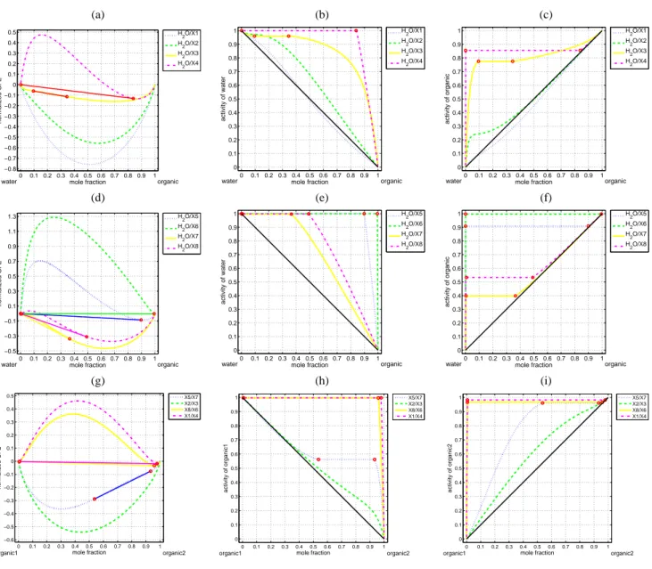
Figures 1a–i show the computed phase diagrams in terms

of the normalized GFE, gn, and equilibrium activities for

bi-nary systems water/X(1–8), X5/X7, X2/X3, X8/X6, X1/X4. The two equilibrium phases are represented by red circles, and are connected by the solid tie-line. In Fig. 1a, for the water/X4 system the two equilibrium phases are located at

organic mole fractions, 1.188 × 10−7and 0.8433 (as listed

in Table 3), corresponding to the two locations at which the Gibbs tangent plane supports the graph of the normalized

GFE. The interval (0, 1.188 × 10−7) on the x-axis

corre-sponds to a one-phase region (not visible in the present scale) that consists of an essentially pure water phase with the

or-ganic mole fraction of X4 less than 1.188 × 10−7. The

in-terval (1.188 × 10−7, 0.8433) on the x-axis corresponds to a

two-phase region where an essentially pure water phase with

the mole fraction of X4 being 1.188 × 10−7_{is in equilibrium}

with an organic phase with the mole fraction of X4 being 0.8433, implying that the water activity in two-phase equi-librium is essentially equal to 1 (refer to Fig. 1b and Table 3). The interval (0.8433, 1) on the x-axis corresponds to a one-phase region that consists of a organic one-phase with the mole fraction of X4 exceeding 0.8433. For the water/X3 system in the same figure, the region where a two-phase equilibrium is predicted by the model, located at the organic mole frac-tions 0.09365 and 0.3453, is smaller compared to the two-phase region for the water/X4 system. On the other hand, no two-phase equilibrium is predicted for the systems of wa-ter/X[1,2]. The activities of components 1 (i.e. water) and 2 (i.e. organic) are shown in Figs. 1b and c.

In Fig. 1d, two-phase equilibria are predicted for all sys-tems water/X(5–8). Phase separation occurs essentially over the entire range for the system water/X6, with the corre-sponding equilibrium water and X6 activities being essen-tially 1 (Table 3, Fig. 1e and Fig. 1f). The two-phase re-gions for the systems water/X(5,7,8) are located in the

inter-vals (2.061 × 10−12, 0.8984), (3.351 × 10−3, 0.3655) and

(1.049 × 10−3, 0.4922), respectively, with the

correspond-ing equilibrium water activity becorrespond-ing essentially 1 (Table 3 and Fig. 1e). In Fig. 1g, phase separation again occurs over

(8)

(a) (b) (c) 0 0.1 0.2 0.3 0.4 0.5 0.6 0.7 0.8 0.9 1 −0.8 −0.7 −0.6 −0.5 −0.4 −0.3 −0.2 −0.1 0 0.1 0.2 0.3 0.4 0.5 mole fraction normalized GFE water organic H 2O/X1 H₂O/X2 H₂O/X3 H 2O/X4 0 0.1 0.2 0.3 0.4 0.5 0.6 0.7 0.8 0.9 1 0 0.1 0.2 0.3 0.4 0.5 0.6 0.7 0.8 0.9 1 mole fraction activity of water water organic H 2O/X1 H₂O/X2 H 2O/X3 H₂O/X4 0 0.1 0.2 0.3 0.4 0.5 0.6 0.7 0.8 0.9 1 0 0.1 0.2 0.3 0.4 0.5 0.6 0.7 0.8 0.9 1 mole fraction activity of organic water organic H 2O/X1 H₂O/X2 H 2O/X3 H₂O/X4 (d) (e) (f) 0 0.1 0.2 0.3 0.4 0.5 0.6 0.7 0.8 0.9 1 −0.5 −0.3 −0.1 0.1 0.3 0.5 0.7 0.9 1.1 1.3 mole fraction normalized GFE water organic H 2O/X5 H₂O/X6 H₂O/X7 H₂O/X8 0 0.1 0.2 0.3 0.4 0.5 0.6 0.7 0.8 0.9 1 0 0.1 0.2 0.3 0.4 0.5 0.6 0.7 0.8 0.9 1 mole fraction activity of water water organic H 2O/X5 H₂O/X6 H₂O/X7 H 2O/X8 0 0.1 0.2 0.3 0.4 0.5 0.6 0.7 0.8 0.9 1 0 0.1 0.2 0.3 0.4 0.5 0.6 0.7 0.8 0.9 1 mole fraction activity of organic water organic H 2O/X5 H₂O/X6 H₂O/X7 H 2O/X8 (g) (h) (i) 0 0.1 0.2 0.3 0.4 0.5 0.6 0.7 0.8 0.9 1 −0.6 −0.5 −0.4 −0.3 −0.2 −0.1 0 0.1 0.2 0.3 0.4 0.5 mole fraction normalized GFE organic1 organic2 X5/X7 X2/X3 X8/X6 X1/X4 0 0.1 0.2 0.3 0.4 0.5 0.6 0.7 0.8 0.9 1 0 0.1 0.2 0.3 0.4 0.5 0.6 0.7 0.8 0.9 1 mole fraction activity of organic1 organic1 organic2 X5/X7 X2/X3 X8/X6 X1/X4 0 0.1 0.2 0.3 0.4 0.5 0.6 0.7 0.8 0.9 1 0 0.1 0.2 0.3 0.4 0.5 0.6 0.7 0.8 0.9 1 mole fraction activity of organic2 organic1 organic2 X5/X7 X2/X3 X8/X6 X1/X4

Fig. 1. Normalized GFE curves for all water/organic systems and two selected organic systems s1/s2, and their respective activities. Equi-librium two phase solutions (if any) are marked with circle symbols. The solid (-) line represents the tie lines. Normalized GFE curves are

plotted as a function of mole fraction of organic component s2for: (a) systems of water (s1)/X[1-4] (s2) at 298.15 K; (b) the activity of

water in systems of water/X[1-4] and (c) activity of X[1-4] for the systems of water/X[1-4]. (d) Systems of water/X[5-8] at 298.15 K. (e) The activity of water in systems of water/X[5-8] and (f) the activity of X[5-8]. (g) Systems of X5/X7, X2/X3, X8/X6, and X1/X4. (h) The

activity of component s1for the s1/s2system is shown in panel (g), and (i) the activity of component s2for the s1/s2system is shown in

panel (h).

almost the entire mole faction range for systems X1/X4 and X8/X6. The corresponding activities for each component in the system are essentially unity (shown in Figs. 1h and i), in-dicating that X1 and X4, X8 and X6 are immiscible with each other. On the other hand, X5 and X7 are partially miscible, and X2 and X3 are fully miscible.

Figure 2 presents phase diagrams for the system water/1-hexacosanol(X5)/pinic acid(X7) at 298.15 K. This system typifies one consisting of a large alkane containing an alco-hol group and an acidic terpene oxidation product, both in

the presence of water. In Fig. 2a, the phase boundaries are marked with solid bold lines, and the dashed lines represent the two-phase tie lines. Three distinct two-phase regions (L2) bordering one three-phase region (L3) are predicted, as shown in Fig. 2a. The third two-phase region, which is a nar-row strip bounded between the bottom edge of the triangular shaped L3 region and the x-axis, is of negligible size and is not visible at the scale of Fig. 2a, but can be deduced from the phase diagram of water/X7 in Fig. 1d. Contours of the ac-tivity of water, 1-hexacosanol, and pinic acid for the mixture

(9)

Table 4. Three-phase equilibrium solutions for ternary systems.

system (s1/s2/s3) (x(1)s2, xs(2)2, xs(3)2) (xs(1)3, x(2)s3, x(3)s3) (as(123)1 , a(123)s2 , a(123)s3 ) (xs(1)2, xs(2)2, xs(3)2) (xs(1)3, x(2)s3, x(3)s3) (as(123)1 , as(123)2 , as(123)3 ) (xs(1)2, x(2)s2, x(3)s2) (xs(1)3, xs(2)3, xs(3)3) (a(123)s1 , as(123)2 , as(123)3 )

water/X1/X[2-8] none none none none none none none none none

water/X3/X4 (8.24e-02, 3.76e-01, 4.78e-01) (7.90e-06, 4.21e-01, 1.17e-02) (9.62e-01, 7.65e-01. 5.79e-01) (7.44e-02, 4.40e-01, 5.43e-01) (9.16e-06, 2.59e-01, 4.93e-02) (9.63e-01, 7.53e-01, 4.77e-01) (4.74e-02, 3.11e-01, 4.62e-01) (6.38e-07, 2.25e-03, 4.80e-01) (9.74e-01, 5.71e-01, 5.72e-01) water/X3/X5 (9.35e-02, 2.65e-01, 3.48e-01) (6.13e-09, 6.16e-01, 4.35e-05) (9.60e-01, 7.75e-01, 6.78e-01) (9.34e-02, 2.78e-01, 3.50e-01) (1.09e-08, 4.69e-01, 7.77e-05) (9.60e-01, 7.75e-01, 4.16e-01) (4.89e-02, 2.84e-01, 5.61e-01) (6.63e-11, 2.92e-05, 3.30e-01) (9.74e-01, 5.74e-01, 3.28e-01) water/X3/X6 (3.86e-02, 9.37e-02, 3.45e-01) (9.59e-01, 8.98e-12, 2.17e-07) (9.60e-01, 7.75e-01, 9.62e-01) (3.86e-02, 9.37e-02, 3.45e-01) (9.59e-01, 8.98e-12, 2.17e-07) (9.60e-01, 7.75e-01, 9.62e-01) (4.90e-02, 2.83e-01, 4.63e-01) (7.81e-14, 3.00e-07, 5.37e-01) (9.74e-01, 5.74e-01, 5.39e-01)

water/X3/X[7,8] none none none none none none none none none

water/X5/X[6] none none none none none none none none none

water/X5/X7 (3.40e-12, 2.33e-03, 6.09e-01) (3.35e-03, 3.72e-01, 2.19e-01) (9.97e-01, 6.71e-01, 3.96e-01) (2.42e-11, 1.81e-04, 5.82e-01) (8.56e-03, 2.09e-01, 1.05e-01) (9.94e-01, 5.11e-01, 1.91e-01) (3.86e-13, 8.46e-04, 4.51e-01) (4.14e-03, 3.55e-01, 4.24e-01) (9.96e-01, 4.81e-01, 4.40e-01) water/X5/X8 (2.06e-12, 1.28e-02, 5.84e-01) (1.03e-03, 5.02e-01, 2.57e-01) (6.85e-01, 5.22e-01, 9.99e-01) (4.95e-12, 6.93e-03, 5.31e-01) (1.54e-03, 3.97e-01, 1.62e-01) (9.99e-01, 4.87e-01, 3.74e-01) (2.20e-13, 9.90e-03, 3.90e-01) (1.06e-03, 5.17e-01, 4.76e-01) (9.99e-01, 5.49e-01, 5.95e-01) water/X6/X7 (2.12e-15, 3.26e-05, 9.87e-01) (3.38e-03, 3.66e-01, 9.66e-03) (9.97e-01, 9.88e-01, 3.98e-01) (7.85e-15, 8.97e-07, 9.93e-01) (8.56e-03, 2.08e-01, 4.57e-03) (9.94e-01, 9.93e-01, 1.91e-01) (2.11e-16, 1.72e-05, 7.67e-01) (4.15e-03, 3.51e-01, 2.28e-01) (9.96e-01, 7.82e-01, 4.41e-01) water/X6/X8 (1.17e-15, 2.72e-04, 9.78e-01) (1.05e-03, 4.93e-01, 1.91e-02) (9.99e-01, 9.80e-01, 5.33e-01) (1.37e-15, 8.73e-05, 9.84e-01) (1.56e-03, 3.90e-01, 1.33e-02) (9.99e-01, 9.85e-01, 3.80e-01) (1.08e-16, 2.72e-04, 8.50e-01) (1.08e-03, 4.99e-01, 1.46e-01) (9.99e-01, 8.74e-01, 6.03e-01)

water/X7/X8 none none none none none none none none none

X{i/j/k}1≤i<j <k≤8none none none none none none none none none

are shown in Figs. 2b, c, and d, respectively. Although no ex-perimental data are available to confirm existence of a three liquid-phase region in this system, three liquid phases are permissible by the Gibbs phase rule and are the most stable equilibrium solution.

For Fig. 2a, if one starts with a mole fraction of 1-hexacosanol of 0.4 and increases the mole fraction of pinic acid from 0 to 0.6 (i.e. going across the phase diagram hori-zontally at a mole fraction of 1-hexacosanol of 0.4), the sys-tem starts within a L2 (two-liquid) region, where the mix-tures separate along the tie-lines into two phases: a mixed or-ganic phase with high concentration of 1-hexacosanol (mole fractions from 0.609 to 0.894), some pinic acid, and water (mole fraction about 0.1), and an almost pure water phase with negligible concentrations of the organics. When the mole fraction of pinic acid is greater than ∼0.16, the L3

region starts, where the mixtures separate into three equi-librium phases: equiequi-librium phase 1 (an almost pure water

phase) with mole fraction of 1-hexacosanol, xs(1)2 =3.40 ×

10−12 and mole fraction of pinic acid xs(1)3 = 0.00335,

equi-librium phase 2 (mixed aqueous phase with 63% of water) with xs(2)2 =0.00233 and x

(2)

s3 =0.372, and equilibrium phase

3 (mixed organic phase dominated by 1-hexacosanol) with

xs(3)2 =0.609 and x

(3)

s3 =0.219 (listed in Table 4). As the mole

fraction of pinic acid passes ∼0.3, the system enters another L2 region with the mixture separating along the tie-lines into two mixed organic phases, one of which includes high con-centrations of both 1-hexacosanol and pinic acid with a small amount of water, and the other of which includes pinic acid and water with a small amount of 1-hexacosanol.

Phase diagrams for the system water/adipic

(10)

(a) (b) 0 0.1 0.2 0.3 0.4 0.5 0.6 0.7 0.8 0.9 1 0 0.1 0.2 0.3 0.4 0.5 0.6 0.7 0.8 0.9 1 L3 L2 L2

mole fraction of 1−hexacosanol

mole fraction of pinic acid

water pinic acid

1−hexacosanol phase diagram

0 0.1 0.2 0.3 0.4 0.5 0.6 0.7 0.8 0.9 0 0.1 0.2 0.3 0.4 0.5 0.6 0.7 0.8 0.9 L3 L2 L2 0.1 0.1 0.2 0.2 0.2 0.3 0.3 0.3 0.3 0.4 0.4 0.4 0.4 0.5 0.5 0.5 0.6 0.6 0.6 0.7 0.7 0.7 0.8 0.8 0.8 0.9 0.9 0.9

water pinic acid

1−hexacosanol activity of water

(c) (d) 0 0.1 0.2 0.3 0.4 0.5 0.6 0.7 0.8 0.9 0 0.1 0.2 0.3 0.4 0.5 0.6 0.7 0.8 0.9 L3 L2 L2 0.3 0.50.4 0.6 0.6 0.6 0.7 0.7 0.8 0.8

water pinic acid

1−hexacosanol activity of 1−hexacosanol

0 0.1 0.2 0.3 0.4 0.5 0.6 0.7 0.8 0.9 0 0.1 0.2 0.3 0.4 0.5 0.6 0.7 0.8 0.9 L3 L2 L2 0.1 0.1 0.2 0.2 0.3 0.3 0.4 0.4 0.5 0.5 0.6 0.6 0.7 0.7 0.8 0.8 0.9 0.9

water pinic acid

1−hexacosanol activity of pinic acid

Fig. 2. Construction of the phase diagram for the system water/1-hexacosanol(X5)/pinic acid(X7) at 298.15 K with tracking of the presence

of each distinct phase region. For each region the boundaries of which are marked with bold lines, the number of liquid phases at equilibrium is represented as L2 for two liquid phases and L3 for three liquid phases. (a) Liquid-liquid equilibrium prediction with two-phase tie lines represented by dashed lines. (b) Labels on the contours (–) indicate the value of the activity of water. (c) Labels on the contours (–) indicate the value of the activity of 1-hexacosanol. (d) Labels on the contours (–) indicate the value of the activity of pinic acid.

model predicts the system to be mostly a one-phase mixture, with a very small two-phase region. A three-phase equilibrium does not exist in this system.

Figure 4 presents the phase diagram for the water/pinonic acid(X8)/nonacosane(X6) system. A three-phase region (L3) is predicted in between three two-phase (L2) regions. Again, a third two-phase region, which is a narrow strip bounded be-tween the left edge of the triangular shaped L3 region and the

y-axis, is of negligible size and is not visible at the scale of

Fig. 4a, but can be deduced from the phase diagram of wa-ter/X8 in Fig. 1d. Figure 5 presents the phase diagram for water/2-hydroxy-glutaric acid(X1)/palmitic acid(X4). The system is predicted to be largely a two-phase mixture, bounded by a small one-phase region at a mole fraction of palmitic acid above 0.85 and a mole fraction of 2-hydroxy-glutaric acid approaching 0 and a one-phase region of

negli-gible size, which is a narrow strip bounded between the left edge of the L2 region and the y-axis, and is not visible at the scale of Fig. 5, but can be deduced from the phase dia-gram of water/X1 in Fig. 1a. There is no three-phase equi-librium predicted for the system. The sensitivity of the pre-dicted phase equilibrium to UNIFAC-Peng and UNIFAC-LL parameters for the ternary system water/1-hexacosanol/pinic acid is illustrated in Figs. 6a and b. By comparing Figs. 6 and 2a, the overall change of the liquid phase equilibrium pre-diction by UNIFAC-Peng and UNIFAC-LL can be assessed. One would expect that UNIFAC-LL should be most accu-rate for the condensed phase calculation in this study, as the UNIFAC-LL parameters have been determined using liquid-liquid equilibrium data. Although UNIFAC parameters were determined using vapor-liquid equilibrium data, it is the most widely used set of parameters, allowing comparison between

(11)

(a) (b) 0 0.1 0.2 0.3 0.4 0.5 0.6 0.7 0.8 0.9 1 0 0.1 0.2 0.3 0.4 0.5 0.6 0.7 0.8 0.9 1 L2

mole fraction of adipic acid

mole fraction of glutaraldehyde

water glutaraldehyde

adipic acid phase diagram

0 0.1 0.2 0.3 0.4 0.5 0.6 0.7 0.8 0.9 0 0.1 0.2 0.3 0.4 0.5 0.6 0.7 0.8 0.9 L2 0.1 0.1 0.1 0.1 0.2 0.2 0.2 0.2 0.3 0.3 0.3 0.3 0.4 0.4 0.4 0.4 0.5 0.5 0.5 0.6 0.6 0.6 0.7 0.7 0.7 0.8 0.8 0.8 0.9 0.9 0.95 0.97

adipic acid activity of water

(c) (d) 0 0.1 0.2 0.3 0.4 0.5 0.6 0.7 0.8 0.9 0 0.1 0.2 0.3 0.4 0.5 0.6 0.7 0.8 0.9 L2 0.1 0.1 0.1 0.2 0.2 0.2 0.3 0.3 0.3 0.4 0.4 0.5 0.5 0.6 0.7 0.8

adipic acid activity of adipic acid

0 0.1 0.2 0.3 0.4 0.5 0.6 0.7 0.8 0.9 0 0.1 0.2 0.3 0.4 0.5 0.6 0.7 0.8 0.9 L2 0.1 0.1 0.2 0.2 0.3 0.3 0.4 0.4 0.5 0.5 0.6 0.6 0.7 0.7 0.8 0.9

adipic acid activity of glutaraldehyde

Fig. 3. Construction of the phase diagram for the system water/adipic acid(X2)/glutaraldehyde(X3) at 298.15 K with tracking of the presence

of each distinct phase region. For each region the boundaries of which are marked with bold lines, the number of liquid phases at equilibrium is represented as L2 for two liquid phases and L3 for three liquid phases. (a) Liquid-liquid equilibrium prediction with two-phase tie lines represented by dashed lines. (b) Labels on the contours (–) indicate the value of the activity of water. (c) Labels on the contours (–) indicate the value of the activity of adipic acid. (d) Labels on the contours (–) indicate the value of the activity of glutaraldehyde.

different models. We return to a more in-depth analysis of the sensitivity to the choice of activity coefficient model in Sect. 5.

4 Effects of organic phase equilibria on inorganic deli-quescence

The inorganic system that has been most widely stud-ied with respect to atmospheric gas-aerosol equilibrium and aerosol state is that of sulfate, nitrate, ammonium, and wa-ter. Particles consisting of these species can be fully aque-ous, fully crystalline, or consist of liquid-solid mixtures, de-pending on the relative concentrations of the components, RH, and temperature. An important question is the extent to which the presence of organic species influences the deli-quescence and efflorescence phase transitions of salts in this system. We now present results of application of UHAERO to computation of the inorganic phase diagram of this sys-tem in the presence of organic species. To construct

del-iquescence phase diagrams of the five-component system

SO2−₄ /NO−₃/NH+₄/H+/H2O, we use the X and Y

compo-sition coordinates as in Amundson et al. (2006c) and define:

X = Ammonium Fraction = b_NH+ 4 b_NH+ 4+bH + , (7) Y = Sulfate Fraction = b_SO2− 4 b_SO2− 4 +b_NO− 3 , (8)

where the system feeds b_SO2−

4 , b_NO− 3, bNH + 4, and bH +are

sub-ject to the constraint of electroneutrality. Thus, for a fixed

(X, Y ) coordinate, we can define a non-unique feed

composi-tion as b_SO2− 4 =_1+YY , b_NO− 3= 1−Y 1+Y, bNH+₄=X, and bH+=1−X. To facilitate the computation of the boundaries in deliques-cence phase diagrams, we also introduce the fractions

f_NH+ 4= b_NH+ 4 b_NH+ 4+bH ++(1 + Y )b_H 2O , (9)

(12)

(a) (b) 0 0.1 0.2 0.3 0.4 0.5 0.6 0.7 0.8 0.9 1 0 0.1 0.2 0.3 0.4 0.5 0.6 0.7 0.8 0.9 1 L3 L2 L2

mole fraction of pinonic acid

mole fraction of nonacosane

water nonacosane

pinonic acid phase diagram

0 0.1 0.2 0.3 0.4 0.5 0.6 0.7 0.8 0.9 0 0.1 0.2 0.3 0.4 0.5 0.6 0.7 0.8 0.9 L3 L2 L2 0.1 0.1 0.2 0.2 0.2 0.3 0.3 0.3 0.4 0.4 0.4 0.5 0.5 0.5 0.6 0.6 0.6 0.7 0.7 0.7 0.8 0.8 0.8 0.9 0.9 0.9

water nonacosane

pinonic acid activity of water

(c) (d) 0 0.1 0.2 0.3 0.4 0.5 0.6 0.7 0.8 0.9 0 0.1 0.2 0.3 0.4 0.5 0.6 0.7 0.8 0.9 L3 L2 L2 0.4 0.5 0.5 0.6 0.6 0.6 0.7 0.7 0.7 0.8 0.8 0.8 0.9 0.9 0.9

water nonacosane

pinonic acid activity of pinonic acid

0 0.1 0.2 0.3 0.4 0.5 0.6 0.7 0.8 0.9 0 0.1 0.2 0.3 0.4 0.5 0.6 0.7 0.8 0.9 L3 L2 L2 0.97 0.97 0.97 0.974 0.974 0.974 0.978 0.978 0.978

water nonacosane

pinonic acid activity of nonacosane

Fig. 4. Construction of the phase diagram for the system water/pinonic acid(X8)/nonacosane(X6) at 298.15 K with tracking of the presence

of each distinct phase region. For each region the boundaries of which are marked with bold lines, the number of liquid phases at equilibrium is represented as L2 for two liquid phases and L3 for three liquid phases. (a) Liquid-liquid equilibrium prediction with two-phase tie lines represented by dashed lines. (b) Labels on the contours (–) indicate the value of the activity of water. (c) Labels on the contours (–) indicate the value of the activity of pinonic acid. (d) Labels on the contours (–) indicate the value of the activity of nonacosane.

f_H+= bH+ b_NH+ 4+bH ++(1 + Y )b_H₂_O , (10)

which, together with fH2O=1−(fNH+₄ + fH+), are the

barycentric coordinates of the unit triangle with vertices

(1 + Y )H2O, NH+₄ and H+. Thus, for a fixed Y , the

frac-tion coordinate (f_NH+ 4, fH +, f_H₂_O) gives X= f NH+₄ f NH+₄+fH+ and bH2O= 1 1+Y f_H2O

1−f_H2O. Therefore, the two-dimensional (2-D)

phase diagrams for fixed Y values can be generated in two

coordinate systems: (X, RH) and (f_H+, f_NH+

4), which can be

chosen on the basis of computational or graphic convenience.

For the system that includes the organic species ORG1,

. . ., ORGno with feeds bORG1, · · ·, bORGno, we introduce the fractions fORG2, . . ., fORGno

fORG2= bORG2 Pno i=1bORGi , · · ·, fORGno= bORGno Pno i=1bORGi , (11)

which, together with fORG1=1−(fORG2+ · · · +fORGno), are

the barycentric coordinates of the (no−1)-dimensional unit

simplex with vertices ORG1, . . . , ORGno. We also need to

specify the organic/inorganic mixing ratio α,

α= Pno i=1bORGi Pni i=1bINORGi+ Pno i=1bORGi , (12) where Pni i=1bINORGi=bNH+₄ + bH++b SO2−₄ +bNO−₃= 2+Y 1+Y. Thus, for a fixed Y , the ratio α and the fraction coordinate

(fORG1, . . . , fORGno) give bORG1=fORG1

α 1−α 2+Y 1+Y, . . ., bORGno=fORGno α 1−α 2+Y 1+Y.

Figures 7a and 7b show the computed phase dia-grams in the (X, RH) coordinate, with tracking of

the presence of each solid phase, for the system

(NH4)2SO4/H2SO4/NH4NO3/HNO3/H2O at 298.15 K and

fixed sulfate fractions Y =1 and 0.85, respectively. For each region of space whose boundaries are marked with bold lines, the existing solid phases at equilibrium are represented,

(13)

(a) (b) 0 0.1 0.2 0.3 0.4 0.5 0.6 0.7 0.8 0.9 1 0 0.1 0.2 0.3 0.4 0.5 0.6 0.7 0.8 0.9 1 L2

mole fraction of 2−hydroxy−glutaric acid

mole fraction of palmitic acid water 2−hydroxy−glutaric acid palmitic acid phase diagram 0 0.1 0.2 0.3 0.4 0.5 0.6 0.7 0.8 0.9 0 0.1 0.2 0.3 0.4 0.5 0.6 0.7 0.8 0.9 L2 0.1 0.1 0.1 0.1 0.2 0.2 0.2 0.2 0.3 0.3 0.3 0.3 0.4 0.4 0.4 0.5 0.5 0.5 0.6 0.6 0.6 0.7 0.7 0.7 0.8 0.8 0.8 0.9 0.9 0.9

mole fraction of palmitic acid water 2−hydroxy−glutaric acid palmitic acid activity of water (c) (d) 0 0.1 0.2 0.3 0.4 0.5 0.6 0.7 0.8 0.9 0 0.1 0.2 0.3 0.4 0.5 0.6 0.7 0.8 0.9 L2 0.1 0.1 0.1 0.2 0.2 0.2 0.3 0.3 0.3 0.4 0.4 0.4 0.5 0.5 0.5 0.6 0.6 0.6 0.6 0.7 0.7 0.7 0.7 0.8 0.8 0.8 0.8 0.9 0.9 0.9

mole fraction of palmitic acid water

2−hydroxy−glutaric acid

palmitic acid activity of 2−hydroxy−glutaric acid

0 0.1 0.2 0.3 0.4 0.5 0.6 0.7 0.8 0.9 0 0.1 0.2 0.3 0.4 0.5 0.6 0.7 0.8 0.9 L2 0.87 0.87 0.87 0.89 0.89 0.89 0.91 0.91 0.91 0.93 0.93 0.93 0.95 0.95 0.95 0.95 0.97 0.97 0.97 0.97

mole fraction of palmitic acid water

2−hydroxy−glutaric acid

palmitic acid activity of palmitic acid

Fig. 5. Construction of the phase diagram for the system water/2-hydroxy-glutaric acid(X1)/palmitic acid(X4) at 298.15 K with tracking

of the presence of each distinct phase region. For each region the boundaries of which are marked with bold lines, the number of liquid phases at equilibrium are represented as L2 for two liquid phases and L3 for three liquid phases. (a) Liquid-liquid equilibrium prediction with two-phase tie lines represented by dashed lines. (b) Labels on the contours (–) indicate the value of the activity of water. (c) Labels on the contours (–) indicate the value of the activity of 2-hydroxy-glutaric acid. (d) Labels on the contours (–) indicate the value of the activity of palmitic acid.

where the seven possible solid phases are labeled as A

through G. A denotes ammonium sulfate, (NH4)2SO4(AS);

B denotes letovicite, (NH4)3H(SO4)2(LET); C denotes

am-monium bisulfate, NH4HSO4 (AHS); D denotes

ammo-nium nitrate, NH4NO3 (AN); E denotes the mixed salt,

2NH4NO3·(NH4)2SO4 (2AN·AS); F denotes the mixed

salt, 3NH4NO3·(NH4)2SO4 (3AN·AS); and G denotes the

mixed salt of ammonium nitrate and ammonium bisulfate,

NH4NO3·NH4HSO4(AN·AHS). In Fig. 7a, for the regions

labeled as AB and BC, the system is fully crystalline and con-sists of the two solid phases A+B and B+C, the mutual deli-quescence RHs of which are 68.57% and 36.65%. In Fig. 7b, for the regions labeled as AB and numbered as 1 through 7, the system consist of aqueous-solid mixtures, where the two solid phases at equilibrium are A+B, A+E, B+E, B+F, B+D, B+G, B+C, and C+G, respectively; for the regions labeled as ABE, BEF, BDF, BDG, BCG, the system is fully crys-talline and consists of the three solid phases A+B+E, B+E+F, B+D+F, B+D+G, B+C+G whose mutual deliquescence RHs are 56.31%, 53.21%, 43.84%, 35.89%, 29.65%. Labels on

the contours (–) present the relative water content in the sys-tem as a function of X and RH. The relative water content is defined as the ratioPnibH2O

i=1bINORGi

of the water content bH2Oat a specific RH and (X,Y ) composition with respect to the

inor-ganic contentPni

i=1bINORGi of the same (X, Y ) composition at the “dry-state”.

For Fig. 7a, if one starts at an ammonium fraction, X=0.6 and increases RH from 0 to 80 (i.e. going up the phase diagram vertically at X=0.6), as represented by the solid red deliquescence curve (a baseline result labeled by (0)) in Fig. 10a, the system starts with a fully crystalline two solid

mixture of B ((NH4)3H(SO4)2) (with 40% of mole fraction)

and C (NH4HSO4) (with 60% of mole fraction). At RH

=36.6%, solid C fully dissolves and the relative water

con-tent in the system promptly takes the value of 0.34, then the system consists of an aqueous electrolyte solution of B and C in liquid-solid equilibrium with solid B, where the relative water content is labeled on the contours in Fig. 7a or given in Fig. 10a. When RH reaches 63.8%, with the relative wa-ter content being 1.44, the system passes the boundary where

(14)

(a) (b) 0 0.1 0.2 0.3 0.4 0.5 0.6 0.7 0.8 0.9 1 0 0.1 0.2 0.3 0.4 0.5 0.6 0.7 0.8 0.9 1 pinic acid water 1−hexacosanol

L3 L2 L2 0 0.1 0.2 0.3 0.4 0.5 0.6 0.7 0.8 0.9 1 0 0.1 0.2 0.3 0.4 0.5 0.6 0.7 0.8 0.9 1 pinic acid water 1−hexacosanol

L3 L2 L2

Fig. 6. Construction of the phase diagram for the system water/1-hexacosanol(X5)/pinic acid(X7) at 298.15 K with two different sets of

UNIFAC parameters: (a) UNIFAC-Peng parameters, (b) UNIFAC-LL parameters.

solid B fully dissolves and the system changes into a single-phase aqueous solution. Similarly for Fig. 7b, as represented by the solid red deliquescence curve (a baseline result labeled by (0)) in Fig. 10b, now with a sulfate fraction Y =0.85, the system starts with a fully crystalline three solid mixture of

B (13.3%) + C (56.7%) + G (NH4NO3·NH4HSO4) (40%) at

X =0.6 and RH =0. At RH =29.7%, solid G fully dissolves

and the relative water content in the system promptly takes the value of 0.19, then the system enters the region labeled 6 in Fig. 7b or labeled BC in Fig. 10b, where the aqueous solu-tion is in liquid-solid equilibrium with two solids B + C. The system passes the boundary at RH =31.6% with the relative water content being 0.29, C dissolves and it is now an aque-ous solution in equilibrium with a single solid B. When RH reaches 58.5%, the relative water content increases to 1.16 and the system becomes a single-phase aqueous solution.

Figures 8 and 9 show the corresponding deliquescence

phase diagrams of (NH4)2SO4/H2SO4/NH4NO3/HNO3/H2O

when the system also includes two organic species, with sulfate fractions (Y ) of 1 and 0.85. In the presence of organic species, the system can exhibit a mixture of multiple liquid and solid phases, depending on the relative composition of inorganic and organic species, RH, and temperature. How-ever, a fully crystalline state of the system is not permissible. Each region that is marked with bold dashed lines delineates the existing liquid phases at equilibrium. The regions of one liquid phase, two liquid phases, and three liquid phases at equilibrium are labeled as L1, L2 and L3, respectively. Labels on the contours represent the relative water content. The bold dashed lines separating different liquid regions are contours of the relative water content taking a value given on the side of the figures.

Figure 8a shows the phase diagram including

1-hexacosanol (ORG1) and pinic acid (ORG2) with the

or-ganic/inorganic mixing ratio α=0.2 and the organic

frac-tions fORG1=0.5 and fORG2=0.5. The molar mixing ratio of

α=0.2 corresponds approximately to the organic/inorganic

mass mixing ratio of 65%. Labels on the contours (–) present

the relative water content (defined as the ratio PnibH2O

i=1bINORGi ) as a function of X and RH. The bold dashed lines separating different liquid regions are contours of the relative water con-tent, with the values of 0.171 and 0.00974. Region L3 covers the fully liquid region and the regions of one solid phase at equilibrium. Region L3 consists of one aqueous phase and two organic phases, where the organic contribution to the ac-tivity of water aw(o)is constant and a(o)w =0.997=1−₁₀₀₀3

(Ta-ble 4, UNIFAC column and water/X5/X7 row). Thus, the locations of contours of the water content in regions L3 are shifted three per thousand in the upward direction, compared to the locations of the corresponding contours in Fig. 7a where the system only includes inorganic species. In the L3 region, the addition of organic species has a negligible effect on the hygroscopic properties of the inorganic electrolytes; the phase diagram and water uptake in this region are almost identical in the presence and absence of organics (Fig. 7a). However, for most of the two solid regions, the phase di-agram and water uptake are quite different as compared to those of the system without organics. L2 covers mostly the two-solids region, and it consists of two liquid (water + or-ganics) phases in equilibrium with two solids (A+B or B+C). The system consists of one liquid (water + organics) phase in equilibrium with two solids in the region that L1 covers. The original fully crystalline phase no longer exists owing to the presence of organics. Also, instead of a straight horizontal line corresponding to the mutual DRH (Fig. 7a), the “deli-quescence” RH is now curved (Figs. 8 and 9). Due to the presence of organics, the originally crystalline system now is in equilibrium with at least one liquid phase. The water con-tent in the system is not negligible and increases with RH. Salts “deliquescence” at a value of RH, with the water con-tent now also a function of the ammonium fraction, causing the curving of the boundaries. If a similar analysis is carried for Fig. 8a as that for Fig. 7a, as represented by the dashed

(15)

(a) (b) 0 0.1 0.2 0.3 0.4 0.5 0.6 0.7 0.8 0.9 1 0 10 20 30 40 50 60 70 80 Water Content Sulfate Fraction Y = 1 T = 298.15 K Ammonium Fraction − X RH (%) _0.05 0.05 0.1 0.1 0.2 0.2 0.2 0.4 0.4 0.8 0.8 0.8 1.2 1.2 1.2 1.6 1.6 1.6 2 2 2.4 2.4 2.8 2.8 3.2 3.2 3.6 3.6 4 4 4 4.4 4.8 5.2 5.6 6 A B C AB BC 0 0.1 0.2 0.3 0.4 0.5 0.6 0.7 0.8 0.9 1 0 10 20 30 40 50 60 70 80 Water Content Sulfate Fraction Y = 0.85 T = 298.15 K Ammonium Fraction − X RH (%) 0.05 0.1 0.2 0.2 0.4 0.4 0.4 0.8 0.8 0.8 1.2 1.2 1.2 1.6 1.6 1.6 2 2 0.1 2.4 2.4 2.8 2.8 3.2 3.2 3.6 3.6 4 4 4 4.4 4.8 4.8 5.2 6 1 2 3 4 5 6 7 A B C AB ABE BEF BDF BDG BCG

Fig. 7. Construction of the phase diagram for the system (NH4)2SO4/H2SO4/NH4NO3/HNO3/H2O with the sulfate fraction: (a) Y =1, (b) Y =0.85, at 298.15 K with tracking of the presence of each phase. For each region the boundaries of which are marked with bold lines, the existing phases at equilibrium are represented. For the regions numbered as 1 through 7, the existing phases at equilibrium are AE, BE, BF, BD, BG, BC, and CG, respectively. Labels on the dashed contours present the relative water content.

green curve and the first row of pie charts (labeled by (1)) in Fig. 10a, the system at X=0.6 starts at RH =0 in a L1 re-gion, where there is a single liquid phase mixed of organics (1-hexacosanol and pinic acid) + little water (as RH is low) with some dissolved ions of B and C in equilibrium with the solids B and C. At RH =6.2%, the system crosses the phase boundary between Ll and L2 (indicated by a dashed line with the relative water content being 9.74e-03), then the system consists of two mixed organic + water phases with some dis-solved ions B and C, and two solid phases B and C that are in equilibrium with the two liquid phases. When the RH reaches 36.5% (a decrease of 0.1 compared to the baseline value of 36.6% in (0)), solid C fully dissolves and the relative water content in the system promptly takes the value of 0.34, then the system crosses the phase boundary between L2 and L3 (indicated by a dashed line with the relative water content being 1.71e-01). Within the L3 region, the system consists of two organic phases (each containing some amount of wa-ter and dissolved ions B and C) and an aqueous phase (with some amount of organics and dissolved ions B and C), which are all in equilibrium with solid B. As RH increases to 63.6% (a decrease of 0.2 compared to the baseline value of 63.8% in (0)), B dissolves and the system is in a three liquid phase equilibrium (two organic phases with some amount of water and dissolved ions and an aqueous phase with some amount of organics and dissolved ions). No solid salt is present in system within the L3 region at a RH >63.6%.

Figure 8b shows the phase diagram with adipic

acid (ORG1) and glutaraldehyde (ORG2) with the

or-ganic/inorganic mixing ratio α=0.2 and the organic fractions

fORG1=0.15 and fORG2=0.85. The model predicts a

two-phase region (L2) in between two L1 regions. Most of the one-solid and all of the two-solids regions are covered by L1; the system consists of a single liquid (water + organics) phase in equilibrium, either with one solid (A, B, or C) or two-solids (A+B, or B+C). L1 covers part of the liquid re-gion, and the system is in a single-phase equilibrium. L2 covers the rest of the liquid region and parts of the one-solid region. There is no L3 region in this system. A slight de-crease of the “deliquescence” RHs for A, B and C can be observed. The “deliquescence” RHs shown in Fig. 8b for A, B and C are ∼77%, ∼66% and ∼34%, while the original val-ues in Fig. 7a are ∼80%, 68.57% and 36.65%. Similarly for Fig. 8b, as represented by the dashed magenta curve and the second row of pie charts (labeled by (2)) in Fig. 10a, the sys-tem at X=0.6 starts at RH =0 in a L1 region, where there is a single liquid phase mixed of organics and water with some dissolved ions of B and C in equilibrium with the solids B and C. At RH = 33.5% (a decrease of 3.1 compared to the baseline value of 36.6% in (0)), solid C fully dissolves and the relative water content in the system reaches 0.34, then the system consists of a single liquid (water + organics + dissolved ions of B and C) phase in equilibrium with solid B. At RH =54.3%, the system crosses the phase boundary between Ll and L2 (indicated by a dashed line with the rela-tive water content being 8.35e-01), then the system consists of two mixed organic + water phases with some dissolved ions B and C in equilibrium with solid B. As RH increases

(16)

(a) (b) 0 0.1 0.2 0.3 0.4 0.5 0.6 0.7 0.8 0.9 1 0 10 20 30 40 50 60 70 80 Water Content Sulfate Fraction Y = 1 T = 298.15 K Ammonium Fraction − X RH (%) 0.05 0.05 0.05 0.1 0.1 0.1 0.2 0.2 0.2 0.4 0.4 0.4 0.8 0.8 0.8 1.2 1.2 1.2 1.6 1.6 1.6 2 2 2 2.4 2.4 2.4 2.8 2.8 3.2 3.2 3.6 3.6 4 4 4 4.4 4.4 4.8 6 _ _ _ _ _ _9.74e−03 L1 _ _ _ _ _ _1.71e−01 L2 L3 A B C AB BC 0 0.1 0.2 0.3 0.4 0.5 0.6 0.7 0.8 0.9 1 0 10 20 30 40 50 60 70 80 Water Content Sulfate Fraction Y = 1 T = 298.15 K Ammonium Fraction − X RH (%) 0.05 0.05 0.05 0.1 0.1 0.1 0.2 0.2 0.2 0.4 0.4 0.4 0.8 0.8 0.8 1.2 1.2 1.2 1.6 1.6 1.6 2 2 0.1 2.4 2.4 0.2 2.8 2.8 3.2 3.2 3.6 3.6 4 4 4 4.4 4.4 4.8 4.8 5.2 5.2 5.6 6 6.4 _ _ _ _ _ _ 8.35e−01 L1 _ _ _ _ _ _2.31e+00 L2 L1 A B C AB BC (c) (d) 0 0.1 0.2 0.3 0.4 0.5 0.6 0.7 0.8 0.9 1 0 10 20 30 40 50 60 70 80 Water Content Sulfate Fraction Y = 1 T = 298.15 K Ammonium Fraction − X RH (%) 0.05 0.05 0.05 0.1 0.1 0.1 0.2 0.2 0.2 0.4 0.4 0.4 0.8 0.8 0.8 1.2 1.2 1.2 1.6 1.6 1.6 2 2 0.1 2.4 2.4 2.4 2.8 2.8 3.2 3.2 3.6 3.6 4 4 4 4.4 4.4 4.8 6 _ _ _ _ _ _1.27e−01 L2 L3 A B C AB BC 0 0.1 0.2 0.3 0.4 0.5 0.6 0.7 0.8 0.9 1 0 10 20 30 40 50 60 70 80 Water Content Sulfate Fraction Y = 1 T = 298.15 K Ammonium Fraction − X RH (%) 0.05 0.05 0.05 0.1 0.1 0.1 0.2 0.2 0.2 0.4 0.4 0.4 0.8 0.8 0.8 1.2 1.2 1.2 1.6 1.6 1.6 2 2 2 2.4 2.4 2.4 2.8 2.8 3.2 3.2 3.6 3.6 4 4 4 4.4 0.2 4.8 4.8 5.2 5.2 6 L2 A B C AB BC

Fig. 8. Construction of the phase diagram for the system (NH4)2SO4/H2SO4/NH4NO3/HNO3/H2O with the sulfate fraction Y =1 at

298.15 K when the system also includes two organic species: (a) 1-hexacosanol (ORG1) and pinic acid (ORG2) with α=0.2, fORG1=0.5

and fORG2=0.5; (b) adipic acid (ORG1) and glutaraldehyde (ORG2) with α=0.2, fORG1=0.15 and fORG2=0.85; (c) pinonic acid (ORG1)

and nonacosane (ORG2) with α=0.2, fORG1=0.5 and fORG2=0.5; (d) 2-hydroxy-glutaric acid (ORG1) and palmitic acid (ORG2) with

α=0.2, f_ORG₁=0.5 and f_ORG₂=0.5.

to 61.4% (a decrease of 2.4 compared to the baseline value of 63.8% in (0)), B dissolves and the system is in a two liq-uid phase equilibrium. No solid salt is present in system at a RH >61.4%. At RH =72.6%, the system crosses the phase boundary between L2 and L1 (indicated by a dashed line with the relative water content being 2.31), then the system is in a single-phase (aqueous phase) equilibrium.

Figure 8c presents the phase diagram with pinonic acid

(ORG1) and nonacosane (ORG2) with the organic/inorganic

mixing ratio α=0.2 and the organic fractions fORG1=0.5 and

fORG2=0.5. The phase diagram for this system is similar to

that of 1-hexacosanol and pinic acid (Fig. 8a). L3 covers fully the liquid region and most of the one-solid regions. L2 covers fully the two-solids region; however, there is no L1 region predicted in this system.

Similarly for Fig. 8c, as represented by the dashed blue curve and the third row of pie charts (labeled by (3)) in

Fig. 10a, the system at X=0.6 starts at RH =0 in a L2 re-gion, where there are two mixed organic + water phases with some dissolved ions B and C, and two solid phases B and C that are in equilibrium with the two liquid phases. When the RH reaches 36.6% (a decrease of 0.04 compared to the baseline value in (0)), solid C fully dissolves and the rela-tive water content in the system promptly takes the value of 0.34, then the system crosses the phase boundary between L2 and L3 (indicated by a dashed line with the relative wa-ter content being 1.27e-01). Within the L3 region, the sys-tem consists of two organic phases (each containing some amount of water and dissolved ions B and C) and an aque-ous phase (with some amount of organics and dissolved ions B and C), which are all in equilibrium with solid B. As RH increases to 63.7% (a decrease of 0.1 compared to the base-line value of 63.8% in (0)), B dissolves and the system is in a three liquid phase equilibrium (two organic phases with

(17)

(a) (b) 0 0.1 0.2 0.3 0.4 0.5 0.6 0.7 0.8 0.9 1 0 10 20 30 40 50 60 70 80 Water Content Sulfate Fraction Y = 0.85 T = 298.15 K Ammonium Fraction − X RH (%) 0.05 0.05 0.05 0.1 0.1 0.1 0.2 0.2 0.2 0.4 0.4 0.4 0.8 0.8 0.8 1.2 1.2 1.2 1.6 1.6 1.6 2 2 2.4 2.4 2.8 2.8 3.2 3.2 3.6 3.6 4 4 4 4.4 4.4 4.8 5.2 5.6 6 _ _ _ _ _ _9.74e−03 L1 _ _ _ _ _ _1.71e−01 L2 L3 2 1 3 4 5 6 7 A B C AB ABE BEF BDF BDG BCG 0 0.1 0.2 0.3 0.4 0.5 0.6 0.7 0.8 0.9 1 0 10 20 30 40 50 60 70 80 Water Content Sulfate Fraction Y = 0.85 T = 298.15 K Ammonium Fraction − X RH (%) 0.05 0.05 0.05 0.1 0.1 0.1 0.2 0.2 0.2 0.4 0.4 0.4 0.8 0.8 0.8 1.2 1.2 1.2 1.6 1.6 1.6 2 2 2 2.4 2.4 2.8 2.8 3.2 3.2 3.6 3.6 4 4 4 4.4 4.4 4.8 4.8 5.2 5.2 5.6 6 6.4 _ _ _ _ _ _8.35e−01 L1 _ _ _ _ _ _2.31e+00 L2 L1 1 2 3 4 5 6 7 A B C AB ABE BEF BDF BDG BCG (c) (d) 0 0.1 0.2 0.3 0.4 0.5 0.6 0.7 0.8 0.9 1 0 10 20 30 40 50 60 70 80 Water Content Sulfate Fraction Y = 0.85 T = 298.15 K Ammonium Fraction − X RH (%) 0.05 0.05 0.05 0.1 0.1 0.1 0.2 0.2 0.2 0.4 0.4 0.4 0.8 0.8 0.8 1.2 1.2 1.2 1.6 1.6 1.6 2 2 2 2.4 2.4 2.4 2.8 2.8 3.2 3.2 3.6 3.6 4 4 4 4.4 4.4 4.8 5.2 5.6 6 _ _ _ _ _ _1.27e−01 L2 L3 1 2 3 4 5 6 7 A B C AB ABE BEF BDF BDG BCG 0 0.1 0.2 0.3 0.4 0.5 0.6 0.7 0.8 0.9 1 0 10 20 30 40 50 60 70 80 Water Content Sulfate Fraction Y = 0.85 T = 298.15 K Ammonium Fraction − X RH (%) 0.05 0.05 0.05 0.1 0.1 0.1 0.2 0.2 0.2 0.4 0.4 0.4 0.8 0.8 0.8 1.2 1.2 1.2 1.6 1.6 1.6 2 2 2 2.4 2.4 2.4 2.8 2.8 3.2 3.2 3.6 3.6 4 4 4 4.4 4.4 4.8 4.8 5.2 5.2 5.6 6 1 2 3 4 5 6 7 A B C AB ABE BEF BDF BDG BCG L2

Fig. 9. Construction of the phase diagram for the system (NH₄)₂SO₄/H₂SO₄/NH₄NO₃/HNO₃/H₂O with the sulfate fraction Y =0.85 at

298.15 K when the system also includes two organic species: (a) 1-hexacosanol (ORG1) and pinic acid (ORG2) with α=0.2, fORG1=0.5

and fORG2=0.5; (b) adipic acid (ORG1) and glutaraldehyde (ORG2) with α=0.2, fORG1=0.15 and fORG2=0.85; (c) pinonic acid (ORG1)

and nonacosane (ORG2) with α=0.2, fORG1=0.5 and fORG2=0.5; (d) 2-hydroxy-glutaric acid (ORG1) and palmitic acid (ORG2) with

α=0.2, fORG1=0.5 and fORG2=0.5.

some amount of water and dissolved ions and an aqueous phase with some amount of organics and dissolved ions). No solid salt is present in system within the L3 region at a RH >63.8%. Figure 8d shows the phase diagram with

2-hydroxy-glutaric acid (ORG1) and palmitic acid (ORG2)

with the organic/inorganic mixing ratio α=0.2 and the

or-ganic fractions fORG1=0.5 and fORG2=0.5. The entire phase

diagram is labeled as a L2 region. A change in the “deliques-cence” RHs of A, B and C can also be observed. The approx-imate values shown in Fig. 8d are 78% for A, 66% for B, and 32% for C, whereas the original values in Fig. 7a are 80%, 68.57%, and 36.65%. Similarly for Fig. 8d, as represented by the dashed cyan curve and the fourth row of pie charts (labeled by (4)) in Fig. 10a, the system at X=0.6 starts at RH

=0 in the L2 region, where there are two mixed organic +

water phases with some dissolved ions B and C in

equilib-rium with the solids B and C. At RH = 27.8% (a decrease of 8.8 compared to the baseline value of 36.6% in (0)), solid C fully dissolves and the relative water content in the system reaches 0.34, then the system consists of two liquid (water + organics + dissolved ions of B and C) phases in equilibrium with solid B. As RH increases to 60.2% (a decrease of 3.6 compared to the baseline value of 63.8% in (0)), B dissolves and the system is in a two liquid phase equilibrium. No solid salt is present in system at a RH >60.2%.

The phase diagrams of (NH4)2SO4/ H2SO4/NH4NO3/

HNO3/H2O for the same four ORG1/ORG2 combinations

are given in Figs. 9a–d, at a fixed sulfate fraction (Y ) of 0.85. Similar to the panels in Fig. 8, the horizontal boundaries cor-responding to the mutual deliquescence RHs for the fully crystalline solid phases in Fig. 7b are now curved in Fig. 9. In the L3 regions of Fig. 9a and c, the addition of organic