Digital holographic imaging of microorganisms

Digital Holographic Imaging of Microorganisms

by

Michael Trevor Wolf

SUBMITTED TO THE DEPARTMENT OF MECHANICAL ENGINEERING IN PARTIAL FULFILLMENT OF THE REQUIREMENTS FOR THE DEGREE OF

BACHELOR OF SCIENCE AT THE

MASSACHUSETTS INSTITUTE OF TECHNOLOGY

JUNE 2006

©2006 Michael Trevor Wolf. All riahts reserved.

MASSACHL OF T1 AUG LIBI JSETS INSTITE ECHNOLOGY 0 2 2006

RARIES

and to distribute publicly paper and electronic copies of this thesis document in whole or in part

in any medium now known or hereafter created.

Signature of Author: Certified by: .

(-

/.

f7r

r Department of Mechanical Engineering

I

1

x

May 12, 2006

·

\

Y --

Accepted by:

,

.

John H. Lienhard V Professor of Mechanical Engineering Chairman, Undergraduate Thesis Committee

ARCHNIES

Digital Holographic Imaging of Microorganisms By

Michael Trevor Wolf

Submitted to the Department of Mechanical Engineering on May 12, 2006 in partial fulfillment of the Requirements for the Degree of Bachelor of Science in

Mechanical Engineering

ABSTRACT

Imaging aquatic microorganisms in 3D space is of interest to biologists and ocean scientists seeking to understand the behavior of these organisms in their natural environments. In this research, digital holographic imaging (DHI), with a 4f system providing transverse magnification of 9.1, is used to study such microorganisms. To test the imaging technique, DHI was used to locate and track 10 micrometer Dunaliella freely swimming in a 30 milliliter tank of artificial ocean water. Multiple holograms were recorded onto one frame with laser pulsing to identify short algae trajectories. An automatic algae locating program was designed, but the signal to noise ratio was too low, and therefore the program could only locate algae reliably with manual confirmation. With refinement to the experimental setup, the signal to noise ratio could be increased, and this imaging technique could be used to analyze many systems of aquatic

microorganisms interacting in a 3D space. Thesis Supervisor: Roman Stocker

Acknowledgements

I would like to thank my thesis advisor, Roman Stocker, for his guidance and ideas, and for giving me the opportunity to work on this project.

I would also like to extend great thanks to Jose Antonio Dominguez-Caballero and Nick Loomis for teaching me a lot about holography. I would not have been able to complete the experiments without their creative ideas and skillful implementation.

I would like to thank Marcos, Justin Seymour, and Tanvir Ahmed for supporting me in the environmental fluidics lab.

Professor Thomas Peacock originally pointed me to this work, and I would like to thank him for that and for his help in my development as a student.

Finally, I would like to thank my mother and father, Chris and Ken, and my entire family for their constant love and support.

1. Introduction

Ocean scientists and biologists are interested in the capability to image microorganisms freely moving in 3D space. Such a capability allows scientists to investigate the interactions of plankton, algae, and bacteria in their natural environments. Digital Holography Imaging (DHI) is a technique that can be used to locate and image such microorganisms as they move about in water. A comparison of the DHI method with other methods of locating and measuring microorganisms can be found in "Digital Holographic Imaging of Aquatic Species" [1].

In DHI, a hologram of the object is recorded onto a charge coupled device (CCD). The hologram can then be reconstructed digitally. In the case of imaging algae, the object is a

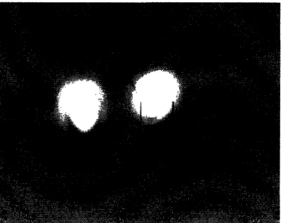
small column of water, sparsely populated with algae. Digital reconstruction allows for the location of many algae in 3 dimensions, and using multiple holograms, trajectories of the algae can be identified. Figure 1 is an intensity map of a digitally reconstructed plane

in three superimposed holograms.

Figure 1: An alga, imaged with 3 superimposed holograms while swimming

freely in a 3D space, is shown in this intensity plot. Its size and velocity are approximately 10 micrometers and 250 micrometers per second.

The purpose of this thesis is to use DHI to identify positions and trajectories of

microorganisms on the 10 um scale. In chapter 2, some theoretical background on DHI is presented. The experimental setup is documented in chapter 3. Post processing

algorithms and the resulting images are presented in chapter 4. Finally, a brief discussion of the implications of this research and recommendations for future work are included in

2. Digital Holographic Imaging

In this chapter, the theoretical basis for the DHI completed in this research is outlined. Section 2.1 is a brief description of in-line holography. In section 2.2, the magnification system used in this research is described theoretically. Multiple exposure holograms are introduced as a way to see microorganism trajectories in section 2.3. Finally, in section 2.4, the necessary mathematics for hologram reconstruction are presented.

2.1 In Line Holography

Holography is an imaging technique in which the interference pattern created by a coherent reference wave and a mutually coherent object wave encodes three dimensional information about the object. A recording of this interference pattern is called a

hologram. In line holography is a name for the original form of holography proposed and first demonstrated by Gabor. The geometry of a Gabor hologram is illustrated in figure 2

[2]. I I Source I I Fl-i i i i L I

L

*1~

(i

'

(1·

Figure 2: Recording geometry for a digital Gabor hologram. The object, which is

transparent, allows a reference wave to pass though it. This reference wave and the scattered light from the object form an interference pattern which is recorded on the CCD, and this recording is called a hologram.

For such a hologram to be recorded, the object must have a high level of average

transmittance, so that in the case of a thin object, the transmitted wave can be represented by the equation,

5

I

t(x,, v,) = t + At(x,,yv,),

where x, and y, are the coordinates on the object plane. Here, t serves as the reference wave and At serves as the object wave [2].

A hologram of a 3D transparent object, such as a tank of water with microorganisms, can be understood as many such thin objects stacked together. Provided that the particles of interest in the water are sparse, the high transmittance of the water allows a strong reference wave to pass though, and the particles of interest in the water can be understood as the At term, which is encoded in the hologram.

A more complete discussion of Gabor holograms, including formal mathematical derivations, can be found in Goodman's Introduction to Fourier Optics [2].

2.2 Magnification with 4f System

This research is concerned with locating and identifying microorganisms on the

micrometer scale. When the microorganisms imaged are as small as or smaller than the pixels used in the CCD, it is necessary to magnify the object while recording the

hologram. Were the image unmagnified, the resolution of the CCD would be insufficient for location of the object.

When a system of lenses is used to magnify a hologram, the hologram recorded is actually a hologram of the image formed by the lenses. Therefore, the relationship of the image location and the object location must be determined in order to map the image to the object. This relationship is determined below.

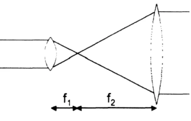
In this research a 4f magnification system was used. Shown in figure 3, a 4f system is composed of 2 lenses with different focal lengths, but which share a focal point.

Figure 3: A 4f system, or a system of 2 lenses which share a focal point,

magnifies and inverts the object. Parallel rays entering the system on the left exit parallel and with a linear scaling. This makes 4f a good choice for holography, because mapping the image space to the object space is simple.

This system provides a transverse magnification of

f:

MT

=

(2.2)

fi

for an object within a plane parallel to the lenses. This can be understood intuitively by using the ray tracing technique shown in figure 3. A ray entering the left lens is inverted

and expanded to exit the right lens at a size proportional to the lens focal length ratio. The longitudinal magnification for the optical system is

ML

=-MT

[3],

(2.3)

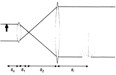
and the location of the image can be found using geometrical optics. As shown in figure 4, an object at a distance s, from lens LI is imaged by LI to sl. The image at sl is the object imaged by lens L2 to focus the final image at si.

So SI S2 Si

Figure 4: A 4f system maps the object space linearly to the image space, with a

different linear scaling for the transverse and longitudinal dimensions.

The longitudinal magnification shown in figure 4 is calculated using geometrical optics. Assuming that the lenses are thin, s is determined by the equation

(2.4)

I I 1

So SI f,

Also, si is determined by

Geometry shows that

algebraically, the value of si is

1 1

1

I

S2 Si f2

Combining and manipulating these equations

f

f

fl

2

For simplification, equation 2.2 is substituted into equation 2.6

Si =-sMT

-MT(fi + f

)'

(2.6)

(2.7) i

This is consistent with the longitudinal magnification value in equation 2.3, and this equation maps the axial location of the image recorded by the CCD to the location of the object. This equation is used in the post processing to locate the microorganisms.

2.3 Finding Trajectories with Multiple Pulses

In order to find trajectories of microorganisms, multiple holograms must be recorded. Because some of the organisms of interest can move at over 10 body lengths per second, recording multiple holograms each second is desirable. However, the CCD used in this research can only record a set of data every 3 seconds. This motivated the use of a multiple exposure technique.

Developed by Dominguez-Caballero and Loomis, the multiple exposure digital holographic imaging (MEDHI) method was used to increase the sampling rate, and therefore to make it possible to determine trajectories of microorganisms swimming in the sampling volume. In the MEDHI method, multiple holograms are recorded in a single frame of the CCD capture by pulsing a coherent source. Then information from each pulse can be digitally reconstructed to locate and identify the microorganism [4]. This is analogous to analyzing a 2D system with multiple exposures recorded on film. MEDHI increases the temporal resolution without the need for a more expensive high speed camera. However, the maximum number of pulses allowable in one frame is limited by the dynamic range of the detector. The DC term increases with each pulse, so the power of each pulse must be reduced accordingly to prevent saturation of the

detector. Additionally, multiple pulses decrease the signal to noise ratio, making the sparsely seeded volume more dense [4].

In these experiments, the multiple pulse technique was used for up to twelve pulses. However, with more than seven pulses, the signal to noise ratio is too high to resolve the images consistently. This will be discussed further in chapter 4.

It is worth noting that a CCD with a higher frame rate could record the same information more dependably, but such a CCD was not available for our research.

2.4 Digital Wavefront Reconstruction

The CCD records the intensity of the superposition between the object and reference waves. This intensity pattern can be described mathematically as

I(x

Ir(x,h yh

o(x,,

.

(2.8)

Here, r(xh,yh) is the reference wave and O(Xh,,y,) is the object wave, and Xh and yh are the coordinates on the CCD plane. This equation is expanded to yield

I(X,',Yh) = r(Xh',yh)l 2+ (XhI,h)12+ r(xh,yh)O* (,,,yh) + r

*

(2.9)

where * denotes a complex conjugate. More mathematical detail and insight into the physical meaning of each of the terms in equation 2.9 is provided in "Digital Holographic Imaging of Aquatic Species" [ 1]. Here, we skip directly to the describing the image reconstruction process.

First, the intensity pattern is multiplied by the digitally generated complex conjugate of the reference wave. This is analogous to shining a physical reference beam on a film hologram. Mathematically, the modified intensity function is

I(XhYh ) r_d (X h X [r(x * ) ,Yh h ) + (XhYh )] (2.

10)

+

r*

As long as the object wave is much weaker than the reference wave, which is coherent and uniform, the combination of the first two terms can be approximated as a DC, or constant term. The third term contains the complex conjugate object field at the CCD plane, multiplied by a constant factor. The fourth term is similar to the third, but actually introduces undesirable artifacts into the image during reconstruction [1].

The next step in reconstructing the hologram is to use the field at the hologram plane to compute the field a distance d from the CCD. This is achieved by convolving the

modified intensity function with the point spread function for the optical system, which is

hy

d ep('

+

d

If the x and y dimensions are sufficiently small compared to the axial dimension d, the Fresnel approximation can be employed, and the point spread function can be simplified to the chirp function

h(x,y,d)= -I exp

x2

(2.12)

Then the field at the reconstruction plane is

E(x,yi)= {1(x,y) hf(x,y,d)}

[1].

(2.13)

This E(xi,yi) is a complex function that includes the magnitude and phase information for the Fresnel approximation of the object wave at the reconstruction plane. For the purpose of visualization of the reconstruction plane, the intensity at the reconstruction plane can be computed:

I(xyi),)=

(xi.yi)

_(2.14)

In actuality, the convolution in equation 2.13 is computed by using a fast Fourier transform on the operands, multiplying in the Fourier domain, and inverse transforming.

3. Imaging of Algae

In this chapter, the experimental realization of the DHI process is described. First, in section 3.1, the equipment used in the imaging system is shown and documented. Section 3.2 includes background information on the dunaliella algae imaged.

3.1 In Line Holography Setup

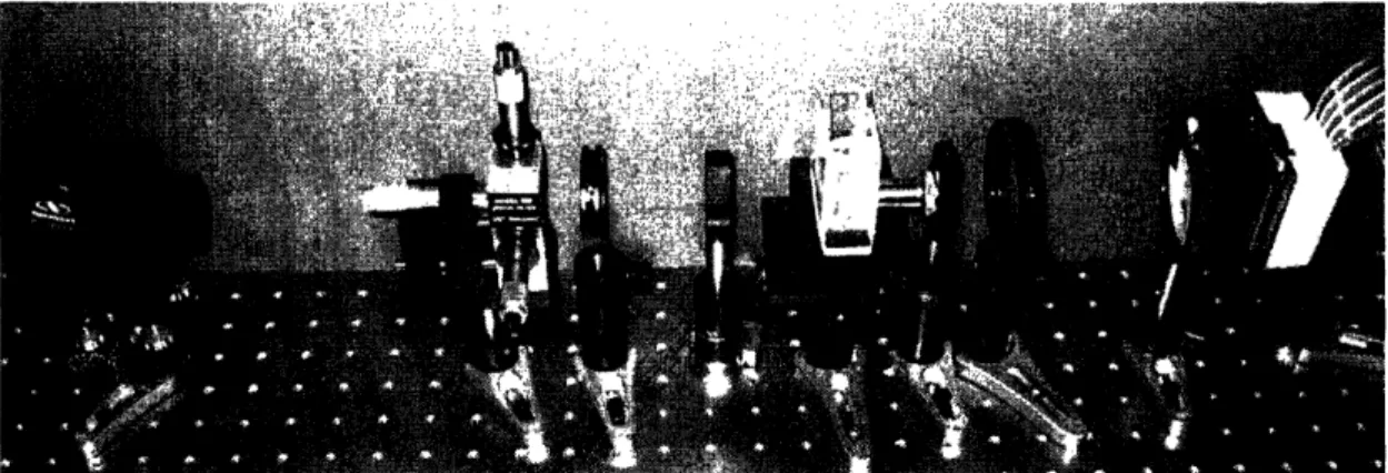
The experimental realization of the in line holography set up with 4f magnification is pictured in figure 5. The sample volume, contained within the glass vessel, is seeded with Dunaliella.

Figure 5: The in-line holography setup. From left to right: laser diode, spacial

filter, pupil, collimating lens, sample, 1Ox objective, pupil, collimating lens. This setup can be more easily understood with the use of the diagram in figure 6, from "Multiple Exposure Immersion Digital Holographic Imaging".

c

''' D

m

-t ; :

~~~~~....

4f ...

LD

SF

CL

Sample

CCD

Figure 6: A diagram of the in line holography setup [4]. The laser diode (LD)

pulses for 100 microseconds. The spatial filter (SF) focuses the light on a pinhole, changing the plane wave into a uniform spherical wave expanding from the pinhole. The collimating lens (CL) provides a uniform plane wave. The wave interacts with the sample and is magnified by the 4f system. Finally, a hologram of the image is recorded by the CCD.

In the following subsections, selected individual components of the system are described in more detail.

3.1.1 Laser

A red laser with a wavelength of 658 nm, a Power Technology PPMT(658-80B), was used in the recording of all holograms presented in this research. The red laser light has been demonstrated to cause minimal disturbance to small aquatic species, when

compared with blue laser light [1]. The laser was pulsed for 100 microsecond intervals with a pulse separation of 250 microseconds in the recording of multiple exposure holograms.

3.1.2 Vessel

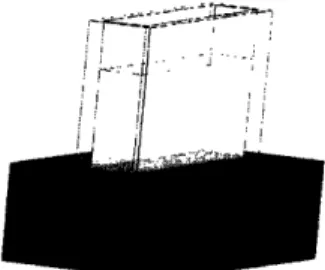
The vessel used in these images was custom built for the application. Shown in figure 7, it has parallel glass walls 22 mm apart in the axial direction. The volume imaged by the magnified holograms was significantly less than the volume of the vessel, but the vessel was designed to be easy to manufacture and clean.

I

l

Figure 7: The sample vessel was a 22 mm x 50 mm by 50 mm glass box with a

machined base and an open top.

In order to reduce the effect of aberrations by the glass, the minimum glass thickness readily available, 2.5 mm, was selected. The light transmitting walls were cleaned with acetone and methanol prior to each experiment.

3.1.3 Magnification with 4f System

The magnification system described in section 2.2 is realized with a 1 OX microscope objective and a lens with a 150 mm focal length. According to the manufacturer, the objective has an effective focal length of 16.5 mm. Therefore, according to equation 2.2, the transverse magnification, M, is -150/16.5 or -9.1. From equation 2.3, the longitudinal magnification is 83.

Though the 10X objective is actually a compound lens, it is approximated as a single lens for simplicity in reconstruction. This approximation introduces some uncertainty in the absolute axial location of the image, but since we are more interested in the relative positions of the algae, this uncertainty is acceptable.

A 20X objective was also used to take some images, the objective introduced too much speckle noise to be useful in imaging algae. Were one available for our research, a higher

quality 20X objective may have yielded images with better signal to noise ratios, and with more easily recognizable images.

3.1.4 CCD

The CCD used for these experiments was a Kodak KAF- 16801 E 16 mega pixel sensor with a pixel pitch of 9 micrometers. The spatial resolution was insufficient in imaging the algae without magnification, and this motivated the use of a 4f system.

The CCD can be exposed for a period of up to 3 seconds, and it takes approximately 1 second to save the data to the computer.

3.2 Dunaliella Tertiolecta Algae

The microorganism imaged in these experiments is the tertiolecta strain of Dunaliella algae. This algae was selected because of its size, swimming speed, and availability. The Dunaliella was grown in F/2 growth media on a 2 week inoculation cycle, and samples for holographic imaging were collected during exponential growth phase.

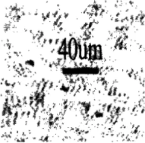
Before taking holographic images, the batch of algae was imaged in a phase contrast microscope with 40X magnification, in order to document its size and swimming speed. The alga has flagella seen in figure 8, as resolved in the microscope, but the flagella are too small to be resolved in the holograms.

Figure 8: Dunaliella imaged with a Nikon Eclipse TE2000-E phase contrast

A video taken with 20X magnification showed that the Dunaliella swam at speeds of approximately 100 to 200 micrometers per second. They reoriented themselves and changed directions several times per second. This behavior was therefore expected in the holograms as well.

The purpose of this research is to develop the DHI system for use in the imaging of microorganisms, rather than to research Dunaliella specifically. For this reason, the information of the size and swimming speed of the algae, as determined with the microscope, was sufficient for completion of the DHI experiments.

4. Identifying Algae Trajectories

With the multiple exposure holograms recorded and saved, the identification of algae trajectories was executed using digital reconstruction of holograms. Because of the great volume of information, a searching algorithm was used to automatically identify possible algae trajectories. However, because of a low signal to noise ratio, manual confirmation was required to find and plot trajectories. In fact, for holograms with more than 3 pulses, the signal to noise ratio was too low for reliable trajectory tracking, even with manual confirmation.

The reconstruction of planes in the image space is described in section 4.1. Section 4.2 is a description of a reference image subtraction technique used to improve image quality. Section 4.3 includes the cross correlation and threshold techniques used to find the algae automatically. Images and plots of algae trajectories are presented in section 4.4.

4.1 Reconstruction of 2D Planes

In order to reconstruct a 2D planes of the image space, the convolution described in equation 2.13 was implemented discretely with MATLAB. The algorithm used in this research was provided by Dominguez-Caballero, and it is documented fully in "Digital Holographic Imaging of Aquatic Species" [1].

4.2 Subtraction of Reference Images

The magnified holograms included a great amount of speckle noise, which caused difficulty in reconstruction and recognition of algae trajectories. A likely cause of this was determined to be the surface roughness of the objective lens. Additional noise was contributed by stationary algae which congregated by the walls of the vessel, and by any particles on the glass.

Because these sources of noise were stationary for the entire duration of the experiment, it is possible to use one hologram as a reference, and to subtract it from the hologram of interest. This reduces the noise, and aids in the identification of algae. However, this technique cannot eliminate noise caused by moving algae, so if the volume is seeded too densely, the signal to noise ratio prevents successful algae identification.

4.3 Identifying Algae Automatically

Because of the volume of data recorded in one hologram, it is desirable to search automatically for algae. However, with our experimental setup, the speckle noise is strong and of similar scale to the algae, so it is difficult to define a reliable criterion to use in finding algae. However, using a cross correlation filter and confirming the validity of the data manually, it was possible to identify some trajectories.

4.3.1 Cross Correlation

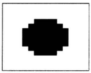
A cross correlation filter was implemented to increase the contrast between the algae and the speckle noise. The filter, pictured in figure 9, is a 16x16 pixel white space with a 10 um diameter blob on the inside. The blob size was selected based on the images of the algae shown in figure 8, in section 3.2.

Figure 9: This shape was cross correlated with the reconstructed planes in order

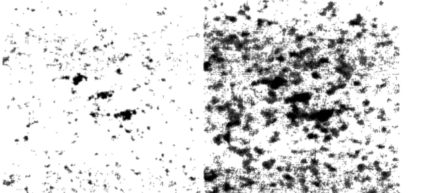
Applying this filter to the image is equivalent mathematically to a cross correlation. Cross correlation of the algae shape with the raw image enhances algae of the same size as the filter, while smoothing the speckle noise. The effects of cross correlation are illustrated in a triple exposure hologram in figure 10. The cross correlation raises the relative intensity of three algae shaped images to sufficient levels for conversion to binary images with a threshold of 0.65 x Imax (x,y), or approximately 2/3 the maximum intensity of the image.

Figure 10: A reconstructed image from a triple exposure hologram. Prior to

processing, a reference hologram was subtracted to reduce noise. From left to right, this is an image of the intensity of the reconstruction, an image of the cross correlation results, and a binary image that shows the blobs that would register as algae.

These 3 images provide a clear trajectory of one alga for the 3 pulse hologram. The cross correlation filter enhances the automatic search capabilities. However, because the speckle noise has similar special frequencies to the algae, it often causes false positives if the threshold is too low. Conversely, many algae are not found if the threshold is set too

high.

4.3.2

Program Architecture

Reconstructing one image plane of 2046x2046 pixels took about 8 seconds, and over 1000 slices are necessary if the entire volume is to be searched at an axial resolution of 10 um. Reconstructing image planes with less pixels is faster, but undesirable, because higher spacial frequency signals contribute to a sharper image in larger slices. For this

17 - ·, r-.-f- ·, ... '"·* '' :"':'"'1" .;4 ·.ra. _-·r·· ,· :'' rb-· ar i··a: · p··:·, r..,. _·e · · .··$iF-· ,· b iak .i: " - r P·· i · . f-*:jt· .::·* r · ,. · ·· *. d,

reason, the searching process was automated to reduce the time to find in focus images of algae.

The steps to finding algae in the program used for this research are briefly outlined here, followed by a more complete description of each step:

* Determine global normalization and threshold values. * Reconstruct image planes in the volume of interest.

* Filter, threshold, and record possible in focus algae positions and focus measure values.

* Compare focus measures of possible algae positions to determine their most likely axial locations.

* Allow the user to confirm findings by presenting a visualization of the data. Prior to a full scan of the data, global normalization parameters are determined. Global normalization parameters are necessary so that intensity values between reconstruction planes could be compared meaningfully. To find global normalization values, some image planes within the volume of interest are reconstructed and filtered, and the maximum and minimum intensity values are recorded. Of these, the overall maximum and minimum intensity values are selected. These are used in normalizing intensity values of each filtered reconstruction plane during the full scan. Threshold values for binary image generation were determined by experimentation with known in-focus algae images.

Next, the full scan begins. This is an iterative process which returns a set of possible algae locations, based on the global normalization and threshold values. The first step in each iteration is to reconstruct an image plane using the convolution approach. This plane is then temporarily available for filtering and conversion to binary.

The second step in each iteration is the cross correlation filter. As described in 4.3.1, the filter enhances the intensity of algae sized images within the reconstructed plane. Then, based on a predetermined threshold, the image plane is converted to binary. Built-in MATLAB functions are used to make groups and to compute the centroid of each group. The locations of these centroids are recorded into a position matrix for later use.

Additionally, the intensity of the cross correlated image at the centroid is recorded, to be used as a focus measure.

Some algae images generate points in the position matrix in multiple reconstruction planes. This is because the slightly out of focus image is present on multiple planes, even though the algae is in focus only on one plane. A 3D plot of these positions is shown in

figure 11.

3p Image Possibilities (um)

6000 5000 4000 3000 2000 1000 0 200 200 0 -400 -600 -600 -400 -200

Figure 11: These are possible algae positions in a triple exposed hologram.

Many points were returned as possible algae positions, including points from blurred algae images on multiple planes. Additional processing is required to eliminate the additional points.

To eliminate double records of the same algae, possible algae positions in the same x and y positions and within 100 um axially are compared, and only the position with the

greatest intensity is confirmed. The filtered data, only including in-focus positions, is shown in figure 12.

19 I'''·

3p In Focus Positions (um) 6000... 5000... 4000 . * *

3000

+

0

-.

200

Figure 12: In-focus positions for the data in figure 11. Note that clusters of

points, which occurred in figure 11 because blurred algae images register on many planes, are compressed into single points here, with the single point representing the in focus image of the algae.

The data in figure 12 is important because each point possibly represents a unique position of an alga. However, the positions must be confirmed manually, because the level of noise makes false registers unavoidable. It is important to note a shortcoming in this process, that two distinct algae images could be mistaken for one in focus algae accompanied by its blurred cluster. Therefore, in a multiple pulse hologram, multiple points for axially moving algae cannot be found.

The last step, manual confirmation, is performed by looking at intensity plots in locations where the position vector contains possible algae. This leads to the data presented in section 4.4.

4.4 Trajectories

Though the low signal to noise ratio prevented the automatic identification of most of the algae trajectories captured in each multiple hologram exposure, it was possible to resolve some trajectories of individual algae. Figure 13 is a 3D plot of the trajectory from the algae shown in a 2D plane in figure 10.

. ...

."

'''''''''"'''''"'''

" ...

....

''.

Figure 13: 3D plot of the trajectory of the algae in figure 10, from a triple pulse

hologram. The units of the plot are micrometers. According to this plot, this algae is moving at about 300 um per second.

It was possible to generate similar plots to that in figure 13 for many algae in the three pulse holograms. Figure 14 is an example of the intensity of an unfiltered reconstruction from a 3 pulse hologram. Note that while each of the algae are imaged in this plane, some of them may be more focused in another reconstruction plane.

some of them may be more focused in another reconstruction plane.

, , , o f,, f ,, ,' wt i .v .r-~ , , ' . f . '

triple hologram pulse _{The algae are moving at about 240 u/second.} . _{Note that}

imaged, slightly

out of focus.

A seven pulse hologram _ii reconstruction plane is shown in figure 15. This figure_{i ;}

lI -t

Figure 1: Filtered inten sity plot of a reconstructd plane in a 7 pulse hologram.

The dark spots in the magnified cluster are most likely an alga moving arou nd at

24 .li4 *11~31

Figure 15: Filtered intensity plot of a reconstructed plane in a 7 pulse hologram.

about 100 micrometers per second, but because of the speckle noise, 7 distinct points cannot be found dependably.

The original intention of this research was to present multiple trajectories generated automatically with a computer program, but this was impossible due to the low signal to noise ratio. However, these images do show that it is possible to resolve trajectories with a magnified DHI setup.

5. Conclusions and Future Direction

This research has shown that it is possible, using in line digital holography with a magnification system, to locate 10 micron algae swimming freely in three dimensions. Furthermore, it is possible to identify short trajectories of the algae by recording multiple holograms in one exposure, though it is difficult to confirm the trajectories with certainty. This imaging method could be applied to many 3D systems of interest to ocean scientists, including population counting, predator prey interactions, and interactions with nutrients. Though we were able to identify some specific algae trajectories with a combination of automatic and manual searching, we were unable to implement an automated program to find and track the algae. Such an implementation is desirable for future research, but the low signal to noise ratio in our holograms prevented it. Therefore, I make two

recommendations for improvement in future research.

First, the magnification system should be improved with a high quality microscope objective. The magnifying lens used for this initial research was a standard 10X objective. A high quality 20X objective, however, would cause less speckle noise, provide more magnification, and give a better signal to noise ratio. Then a computer program could be used to automatically count, identify, and plot the positions of microorganisms

Additionally, taking multiple holograms with a high frame rate CCD, rather using a pulsed laser to record multiple holograms on one frame, would allow for the unique identification of trajectories, because there would not be uncertainty in the temporal

location of an in focus microorganism. Single pulse captures also have a better signal to noise ratio, so the microorganisms would be easier to automatically recognize.

With these improvements, a DHI system could provide much useful information for ocean scientists and microbiologists interested in aquatic microorganisms.

References:

[1] J.A. Dominguez-Caballero, "Digital Imaging of Aquatic Species," MIT Master of

Science in Mechanical Engineering thesis, 2005.

[2] J.W. Goodman, "Introduction to Fourier Optics," Roberts and Company Publishers,

Greenwood Village, CO, Third Edition, 2005.

[3] E. Hecht, "Optics," Addison Wesley, San Francisco, CA, 2002.

[4] J.A. Dominguez-Caballero et al., "Multiple Exposure Immersion Digital Holographic

Imaging," submitted to Conference on Lasers and Electro-Optics (CLEO), 2006.