Submitted to Proceedings of the SIGMOD "98 Conference
DIRECT: Disovering and Reconciling
Conflicts for Data Integration
Hongjun Lu, Weiguo Fan, Cheng Hian Goh,
Stuart E. Madnick, David W. Cheung
Sloan WP #3999
CISL WP #98-02
January 1998
The Sloan School of Management
Massachusetts Institute of Technology
Paper No: 109
DIRECT: Discovering and Reconciling Conflicts
for Data Integration
Hongjun Lu
Weiguo Fan
Cheng Hian Goh
Department of Information Systems & Computer Science
National University of Singapore
{luhj,fanwgu,gohch} @iscs.nus.sg
Stuart E. Madnick
David W. Cheung
Sloan School of Mgt
Dept of Computer Science
MIT
Hong Kong University
[email protected]
[email protected]
Abstract
The successful integration of data from autonomous and heterogeneous systems calls for the prior identifi-cation and resolution of semantic conflicts that may be present. Traditionally, this is manually accomplished by the system integrator, who must sift through the data from disparate systems in a painstaking manner.
We suggest that this process can be partially automated by presenting a methodology and technique for the discovery of potential semantic conflicts as well as the underlying data transformation needed to resolve the conflicts. Our methodology begins by classifying data value conflicts into two categories: context independent
and context dependent. While context independent conflicts are usually caused by unexpected errors, the context
dependent conflicts are primarily a result of the heterogeneity of underlying data sources. To facilitate data in-tegration, data value conversion rules are proposed to describe the quantitative relationships among data values involving context dependent conflicts. A general approach is proposed to discover data value conversion rules from the data. The approach consists of the five major steps: relevant attribute analysis, candidate model selec-tion, conversion function generaselec-tion, conversion function selection and conversion rule formation. It is being implemented in a prototype system, DIRECT, for business data using statistics based techniques. Preliminary study using both synthetic and real world data indicated that the proposed approach is promising.
1 Introduction
The exponential growth of the Internet has resulted in huge quantities of data becoming available. Throngs of au-tonomous systems are routinely deployed on the World Wide Web, thanks in large part to the adoption of the HTTP protocol as a de facto standard for information delivery. However, this ability to exchange bits and bytes, which we call physical connectivity, does not automatically lead to the meaningful exchange of information, or logical
connectivity. The quest for semantic interoperability among heterogeneous and autonomous systems (Sheth & Larson 1990) is the pursuit of this form of logical connectivity.
Traditional approaches to achieving semantic interoperability can be identified as either tightly-coupled or
loosely-coupled (Scheuermann, Yu, Elmagarmid, Garcia-Molina, Manola, McLeod, Rosenthal & Templeton Dec
1990). In tightly-coupled systems, semantic conflicts are identified and reconciled a priori in one or more shared schema, against which all user queries are formulated. This is typically accomplished by the system integrator or DBA who is responsible for the integration project. In a loosely-coupled system, conflict detection and resolution is the responsibility of users, who must construct queries that take into account potential conflicts and identify operations needed to circumvent them. In general, conflict detection and reconciliation is known to be a difficult and tedious process since the semantics of data are usually present implicitly and often ambiguous. This problem poses even greater difficulty when the number of sources increases exponentially and when semantics of data in underlying sources changes over time.
The Context Interchange framework (Goh, Bressan, Madnick & Siegel 1996, Bressan, Fynn, Goh, Jakobisiak, Hussein, Kon, Lee, Madnick, Pena, Qu, Shum & Siegel 1997) has been proposed to provide support for infor-mation exchange data among heterogeneous and autonomous systems. The basic idea is to partition data sources (databases, web-sites, or data feeds) into groups, each of which shares the same context, the latter allowing the semantics of data in each group to be codified in the form of meta-data. A context mediator takes on the responsi-bility for detecting and reconciling semantic conflicts that arise when information is exchanged between systems (data sources or receivers). This is accomplished through the comparison of the contexts associated with sources and receivers engaged in data exchange (Bressan, Goh, Madnick & Siegel 1997).
As attractive as the above approach may seem, it requires data sources and receivers participating in informa-tion exchange to provide the required contexts. In the absence of other alternatives, this codificainforma-tion will have to be performed by the system integrator. This however is a arduous process, since data semantics are not always explicitly documented, and often evolves with the passage of time (a prominent example of which is the Year 2000 problem).
The concerns just highlighted form the primary motivation for the work reported in this paper. Our goal is to develop a methodology and associated techniques that assists in uncovering potential disparities in the way data is represented or interpreted, and in so doing, assists in the codification of contexts associated with different data sources. The success of our approach will make the Context Interchange approach all the more attractive since it means that contextual information will be more easily available.
Our approach is distinct from previous efforts in the study of semantic conflicts in various ways. First, we begin with a simpler classification scheme of conflicts presented in data values. We classify such conflicts into two categories: context dependent and context independent. While context dependent conflicts are a result of disparate interpretations inherent in different systems and applications, context independent conflicts are often caused by errors and external factors. As such, context dependent conflicts constitute the more predictable of the two and can often be rectified by identifying appropriate data value conversion rules, or simply conversion rules, which we will shortly define. These rules can either be used to generate context for different data sources, or be used for data exchange or integration directly.
The conversion rules which are alluded to above can be provided by information providers (or system inte-grators) who have intimate knowledge of the systems involved and who are domain experts in the underlying application domain. We propose in this paper an approach that "mines" such rules from data themselves. The approach requires a training data set consisting of tuples merged from data sources to be integrated or exchanged. Each tuple in the data set should represent a real world entity and its attributes (from multiple data sources) model the properties of the entity. If semantic conflicts exist among the data sources, the values of those attributes that model the same property of the entity will have different values. A mining process first identifies attribute sets each of which involves some conflicts. After identifying the relevant attributes, models for possible conversion functions, the core part of conversion rules are selected. The selected models are then used to analyze the data
to generate candidate conversion functions. Finally, a set of most appropriate functions are selected and used to form the conversion rules for the involved data sources.
The techniques used in each of the above steps can vary depending on the property of data to be integrated. In this paper, we describe a statistics-based prototype system for integrating financial and business data, DIRECT (DIscovering and REconciling ConflicTs). The system uses partial correlation analysis to identify relevant attributes, Bayesian information criterion for candidate model selection, and robust regression for conversion function generation. Conversion function selection is based on the support of rules. Experiment conducted using a real world data set indicated that the system successfully discovered the conversion rules among data sources containing both context dependent and independent conflicts.
The contributions of our work are as follows. First, our classification scheme for semantic conflicts is more practical than previous proposals. For those context dependent conflicts, proposed data value conversion rules can effectively represent the quantitative relationships among the conflicts. Such rules, once defined or discovered, can be used in resolving the conflicts during data integration. Second, a general approach for mining the data conversion rules from actual data values is proposed. The approach can be partially (and in some cases, even fully) automated. Our proposal has been implemented in a prototype system and preliminary findings has been promising.
The remainder of the paper is organized as follows. In Section 2, we suggest that conflicts in data values can be categorized into two groups. We show that (data value) conversion rules can be used to describe commonly-encountered quantitative relationships among data gathered from disparate sources. Section 3 describes a general approach aimed at discovering conversion rules from actual data values. A prototype system that implements the proposed approach using statistical techniques is described in Section 4. Experience with a set of real world data using the system is discussed in Section 5. Finally, Section 6 concludes the paper with discussions on related and future work.
2 Data value conflicts and conversion rules
In this section, we propose a typology for data value conflicts encountered in the integration of heterogeneous and autonomous systems. Specifically, we suggest that these conflicts can be classified into two groups, context
de-pendent conflicts and context indede-pendent conflicts. While context indede-pendent conflicts are highly unpredictable
and can only be resolved by ad hoc methods, context dependent conflicts represent systematic disparities which are consequences of disparate contexts. In many instances, these conflicts involve data conversions of a quantita-tive nature: this presents opportunities for introducing data conversion rules that can be used for facilitating the resolution of these conflicts.
2.1 Data value conflicts
To motivate our discussion, we begin with an example of data integration. A stock broker produces daily stock report for its clients based on the daily quotation of stock prices. Information on stock prices and the report can be represented by relations stock and stkrpt respectively:
stock (stock, currency, volume, high, low, close); stkrpt (stock, price, volume, value);
Table 1 lists sample tuples from the two relations. Since we are primarily concerned with data value conflicts in this study, we assume that the schema integration problem and the entity identification (Wang & Madnick 1989)
Table 1: Example tuples from relation stock and stk rpt
stock stk.rpt
stock currency volume high low close
100 1 438 100.50 91.60 93.11 101 3 87 92.74 78.21 91.35 102 4 338 6.22 5.22 5.48 104 1 71 99.94 97.67 99.04 111 0 311 85.99 70.22 77.47 115 2 489 47.02 41.25 41.28 120 3 370 23.89 21.09 22.14 148 3 201 23.04 19.14 21.04 149 1 113 3.70 3.02 3.32
problem are largely solved. Therefore, it is understood that both stkrpt.price and stock.close are the closing price of a stock of the day. Similarly, both stock.volume and stkrpt.volume are the number of shares traded during the day. Furthermore, it is safe to assume that two entries with the same key (stock) value refer to the same company's stock. For example, tuple with stock = 100 in relation stock and tuple with stock = 100 in relation
stk rpt refer to the same stock.
With these assumptions, it will be reasonable to expect that, for a tuple sis E stock and a tuple tit E stk rpt, if s.stock = t.stock, then s.close = t.price and s.volume = t.volume. However, from the sample data, this does not hold. In other words, data value conflicts exist among two data sources. In general, we can define data value conflicts as follows.
Definition Given two data sources DS1 and DS2 and two attributes A1and A2modeling the same property of a real world entity type in DS1 and DS2 respectively, if t E DS1 and t2 E DS2 represent the same real world instance of the object but t1.A10 t2 .A2, then we say that a data value conflict exists between DS1 and DS2.
In the above definition, attributes A1 and A2are often referred as semantically equivalent attributes and the conflicts defined are referred as semantic conflicts. We refer to these simply as value conflicts since it is some-times rather difficult to decouple conflicts caused by differences in structures from those resulting from semantic differences (Chatterjee & Segev 1991). It is generally agreed that structural conflicts occur when the attributes are defined differently in different databases. Typical examples include type mismatch, different formats, units, and granularity. Semantic incompatibility occurs when similarly defined attributes take on different values in dif-ferent databases, including synonyms, homonyms, difdif-ferent coding schemes, incomplete information, recording errors, different system generated surrogates and synchronous updates. Examples of these have been described by Kashyap and Sheth, who has provided a classification of the various incompatibility problems in heterogeneous databases (Kashyap & Sheth 1996). According to their taxonomy, naming conflicts, data representation conflicts, scaling conflicts, precision conflicts are classified as domain incompatibility problem, data inconsistency and inconsistency caused by different database states are classified as data value incompatibilities.
While a detailed classification of various conflicts or incompatibility problems may be of theoretical impor-tance to some, it is also true that over-classification may introduce unnecessary complexity that are not useful for finding solutions to the problem. We adopt instead the Occam' s razor in this instance and suggest that data value conflicts among data sources can be classified into two categories: context dependent and context independent. Context dependent conflicts exist because data from different sources are stored and manipulated under
differ-stock price volume value
100 65.18 438000 28548840.00 101 164.43 87000 14305410.00 102 31.78 338000 10741640.00 104 69.33 71000 4922430.00 111 30.99 311000 9637890.00 115 41.28 489000 20185920.00 120 39.85 370000 14744500.00
]
---ent context, defined by the systems and applications, including physical data repres---entation and database design considerations. Most conflicts mentioned above, including different data type and formats, units, and granularity, synonyms, different coding schemes are context dependent conflicts. On the other hand, context independent conflicts are those conflicts caused by somehow random factors, such as erroneous input, hardware and software malfunctions, asynchronous updates, database state changes caused by external factors, etc. It can be seen that context independent conflicts are caused by poor quality control at some data sources. Such conflicts would not exist if the data are "manufactured" in accordance to the specifications of their owner. On the contrary, data values involving context dependent conflicts are perfectly good data in their respective systems and applications.
The rationale for our classification scheme lies in the observation that the two types of conflicts command dif-ferent strategies for their resolution. Context independent conflicts are more or less random and non-deterministic, hence it is almost impossible to find mechanisms to resolve them systematically or automatically. For example, it is very difficult, if not impossible, to define a mapping which can correct typographical errors. Human inter-vention and ad hoc methods are probably the best strategy for resolving such conflicts. On the contrary, context dependent conflicts have more predictable behavior. They are uniformly reflected among all corresponding real world instances in the underlying data sources. Once a context dependent conflict has been identified, it is possible to establish some mapping function that allows the conflict to be resolved automatically. For example, a simple unit conversion function can be used to resolve scaling conflicts, and synonyms can be resolved using mapping tables.
2.2 Data value conversion rules
In this subsection, we define data value conversion rules (or simply conversion rules) which are used for describ-ing quantitative relationships among the attribute values from multiple data sources. For ease of exposition, we shall adopt the notation of Datalog for representing these conversion rules. Thus, a conversion rule takes the form
head +- body.
The head of the rule is a predicate representing a relation in one data source. The body of a rule is a conjunction of a number of predicates, which can either be extensional relations present in underlying data sources, or builtin predicates representing arithmetic or aggregate functions. Some examples of data conversion rules are described below.
Example: For the example given at the beginning of this section, we can have the following data value conversion rule:
stkrpt(stock, price, volume, value)
+-exchange-rate(currency, rate), stock(stock, currency, volumeinlK, high, low, close), price = close * rate, volume = volumeinK * 1000, value = price * volume.
Example: For conflicts caused by synonyms or different representations, it is always possible to create lookup tables which forms part of the conversion rules. For example, to integrate the data from two relations
Dl.student(sid, sname, major) and D2.employee(eid, ename, salary), into a new relation Dl.stdemp(id, name,
major, salary), we can have a rule
Dl.stdemp(id, name, major salary)
where sameperson is a relation that defines the correspondence between the student id and employee id. Note that, when the size of the lookup table is small, it can be defined as rules without bodies. One widely cited example of conflicts among student grade points and scores can be specified by the following set of rules:
Dl.student(id, name, grade) +- D2.student(id, name, score), scoregrade(score, grade). score-grade(4, 'A').
score-grade(3, 'B'). score-grade(2, 'C'). score-grade(l, 'D'). score-grade(O, 'F').
One important type of conflicts mentioned in literature in business applications is aggregation conflict (Kashyap & Sheth 1996). Aggregation conflicts arise when an aggregation is used in one database to identify a set of entities in another database. For example, in a transactional database, there is a relation sales(date,
cus-tomer; part, amount) that stores the sales of parts during the year. In an executive information system, relation salessummary(part, sales) captures total sales for each part. In some sense, we can think sales in relation salessummary and amount in sales are attributes with the same semantics (both are the sales amount of a
particular part). But there are conflicts as the sales in salessummary is the summation of the amount in the
sales relation. To be able to define conversion rules for attributes involving such conflicts, we can extend the
traditional datalog to include aggregate functions. In this example, we can have the following rules
salessummary(part, sales) +- sales(date, customer part, amount), sales = SUM(part, amount).
where SUM(part, amount) is an aggregate function with two arguments. Attribute part is the group - by attribute and amount is the attribute on which the aggregate function applies. In general, an aggregate function can take n + 1 attributes where the last attribute is used in the aggregation and others represent the "group-by" attributes. For example, if the salessummary is defined as the relation containing the total sales of different parts to different customers. The conversion rule could be defined as follows:
salessummary(part, customer sales)
-sales(date, customer part, amount), sales = SUM(part, customer amount).
We like to emphasize that it is not our intention to argue about appropriate notations for data value conversion rules and their respective expressive power. For different application domains, the complexity of quantitative relationships among conflicting attributes could vary dramatically and this will require conversion rules having different expressive power (and complexity). The research reported here is primarily driven by problems reported for the financial and business domains; for these types of applications, a simple Datalog-like representation has been shown to provide more than adequate representations. For other applications (e.g., in the realm of scientific data), the form of rules could be extended. Whatever the case may be, the framework set forth in this paper can be used profitably to identify conversion rules that are used for specifying the relationships among attribute values involving context dependent conflicts.
3 Discovering data value conversion rules from data
Data value conversion rules among data sources are determined by the original design of the data sources involved. Although it seems reasonable to have owners of the data sources provide such information, this is difficult to
achieve in practice. While the Internet and the World Wide Web have rendered it easy to obtain data, metadata needed for the correct interpretation of information originating from disparate sources are not easily available. To certain extent, metadata are a form of asset to information providers, especially when it involves value-added processing of raw data. This situation is further aggravated by the fact that databases evolve over time and the meaning of data present in there may change as well. These observations point to the need for more effective means of discovering (or mining) data value conversion rules from the data themselves.
Recall that there are essentially two information components in a data conversion rule: the schema informa-tion, i.e., the relations and their attributes, and the mappings ("function") that describes how an attribute may be derived from one or more of the others. We refer to the latter as conversion functions in the rest of our discussion. It is obvious that, a core task of mining data value conversion rules is to mine the conversion functions. With conversion functions, the conversion rules can be formed without much difficulty.
Figure 1: Discovering data value conversion rules from data
Figure 1 depicts the reference architecture of our approach to discover data value conversion rules from data. The system consists of two subsystems: Data Preparation and Rule Mining. The data preparation subsystem prepares a data set - the training data set - to be used in the rule mining process. The rule mining subsystem analyzes the training data to generate candidate conversion functions. The data value conversion rules are then formed using the selected conversion functions.
3.1
Training data preparation
The objective of this subsystem is to form a training data set to be used in the subsequent mining process. Recall our definition of data value conflicts. We say two differing attributes values tl .A1and t2.A2from two data sources
DS1, tl E DS1and DS2, t2 E DS2 are in conflict when 1. t and t2 represent the same real world entity; and
2. Al and A2 model the same property of the entity.
The training data set should contain a sufficient number of tuples from two data sources with such conflicts. To determine whether two tuples t, t E DS1 and t2, t2 E DS2 represent the same real world entity is an
entity identification problem. In some cases, this problem can be easily resolved. For example, the common keys
of entities, such as a person' s social security number and a company' s registration number, can be used to identify the person or the company in most of the cases. However, in large number of cases, entity identification is still a rather difficult problem (Lim, Srivastava, Shekhar & Richardson 1993, Wang & Madnick 1989).
To determine whether two attributes Al and A2in t and t2 model the same property of the entity is one sub-problem of schema integration, the attribute equivalence sub-problem. Schema integration has been quite well studied in the context of heterogeneous and distributed database systems (Chatterjee & Segev 1991, Larson, Navathe & Elmasri 1989, Litwin & A.Abdellatif 1986). One of the major difficulties to identify equivalent attributes is that such equivalence cannot be simply determined by the syntactic or structural information of the attributes. Two attributes modeling the same property may have different names and different structures but two attributes modeling different properties can have the same name and same structures.
In our study, we will not address the entity identification problem and assume that the data to be integrated have common identifiers so that tuples with the same key represent the same real world entity. This assumption is not unreasonable if we are dealing with a specific application domain. Especially for training data set, we can verify the data manually in the worst case. As for attribute equivalence, as we can see later, the rule mining process has to implicitly solve part of the problem.
3.2 Data value conversion rule mining
Like any knowledge discovery process, the process of mining data value conversion rules is a complex one. More importantly, the techniques to be used could vary dramatically depending on the application domain and what is known about the data sources. In this subsection, we will only briefly discuss each of the modules. A specific implementation for financial and business data based on statistical techniques will be discussed in the next section. As shown in Figure 1 the rule mining process consists of the following major modules: Relevant Attribute
Analysis, Candidate Model Selection, Conversion Function Generation, Conversion Function Selection, and Con-version Rule Formation. In case no satisfactory conCon-version functions are discovered, training data is reorganized
and the mining process is re-applied to confirm that there indeed no functions exist. The system also tries to learn from the mining process by storing used model and discovered functions in a database to assist later mining activities.
3.2.1 Relevant attribute analysis
The first step of the mining process is to find sets of relevant attributes. These are either attributes that are seman-tically equivalent or those required for determining the values of semanseman-tically equivalent attributes. As mentioned earlier, semantically equivalent attributes refer to those attributes that model the same property of an entity type. In the previous stock and stkrpt example, stock.close and stkxrpt.price are semantically equivalent attributes because both of them represent the last trading price of the day. On the other hand, stock.high (stock.low) and
stk rpt.price are not semantically equivalent, although both of them represent prices of a stock, have the same
data type and domain.
The process of solving this attribute equivalence problem can be conducted at two levels: at the metadata level or at the data level. At the metadata level, equivalent attributes can be identified by analyzing the available metadata, such as the name of the attributes, the data type, the descriptions of the attributes, etc. DELTA is an example of such a system (Benkley, Fandozzi, Housman & Woodhouse 1995). It uses the available metadata about attributes and converts them into text strings. Finding corresponding attributes becomes a process of searching for similar patterns in text strings. Attribute equivalence can also be discovered by analyzing the data. An example of such a system is Semlnt (Wen-Syan Li 1994), where corresponding attributes from multiple databases are identified by analyzing the data using neural networks. In statistics, techniques have been developed to find correlations among variables of different data types. In our implementation described in the next section, partial correlation analysis is used to find correlated numeric attributes. Of course, equivalent attributes could be part of available metadata. In this case, the analysis becomes a simple retrieval of relevant metadata.
In addition to finding the semantically equivalent attributes, the relevant attributes also include those attributes required to resolve the data value conflicts. Most of the time, both metadata and data would contain some useful information about attributes. For example, in relation stock, the attribute currency in fact contains certain infor-mation related to attributes low, high and close. Such informative attributes are often useful in resolving data value conflicts. The relevant attribute sets should also contain such attributes.
3.2.2 Conversion function generation
With a given set of relevant attributes, {A1, ...Ak, B1, ...B} with A1and B1being semantically equivalent at-tributes, the conversion function to be discovered
Al = f (B1, B..., BA2, ..., Ak) (1) should hold for all tuples in the training data set. The conversion function should also hold for other unseen data from the same sources. This problem is essentially the same as the problem of learning quantitative laws from the given data set, which has been a classic research area in machine learning. Various systems have been reported in the literature, such as BACON (Langley, Simon, G.Bradshaw & Zytkow 1987), ABACUS (Falkenhainer & Michalski 1986), COPER (Kokar 1986), KEPLER (Wu & Wang 1991), FORTY-NINER (Zytkow & Baker 1991). Statisticians have also studied the similar problem for many years. They have developed both theories and sophis-ticated techniques to solve the problems of associations among variables and prediction of values of dependent variables from the values of independent variables.
Most of the systems and techniques require some prior knowledge about the relationships to be discovered, which is usually referred as models. With the given models, the data points are tested to see whether the data fit the models. Those models that provide the minimum errors will be identified as discovered laws or functions. We divided the task into two modules, the candidate model selection and conversion function generation. The first module focuses on searching for potential models for the data from which the conversion functions are to be discovered. Those models may contain certain undefined parameters. The main task of the second module is to have efficient algorithms to determine the values of the parameters and the goodness of the candidate models in these models. The techniques developed in other fields could be used in both modules. User knowledge can also be incorporated into the system. For example, the model base is used to store potential models for data in different domains so that the candidate model selection module can search the database to build the candidate models.
3.2.3 Conversion function selection and conversion rule formation
It is often the case that the mining process generates more than one conversion functions because it is usually difficult for the system to determine the optimal ones. The conversion function selection module needs to de-velop some measurement or heuristics to select the conversion functions from the candidates. With the selected functions, some syntactic transformations are applied to form the data conversion rules as specified in Section 2.
3.2.4 Training data reorganization
It is possible that no satisfactory conversion function is discovered with a given relevant attribute set because no such conversion function exists. However, there is another possibility from our observations: the conflict cannot be reconciled using a single function, but is reconcilable using a suitable collection of different functions. To accommodate for this possibility, our approach includes a training data reorganization module. The training data set is reorganized whenever a single suitable conversion function cannot be found. The reorganization process usually partitions the data into a number of partitions. The mining process is then applied in attempting to identify appropriate functions for each of the partition taken one at a time. This partitioning can be done in a number of different ways by using simple heuristics or complex clustering techniques. In the case of our implementation (to be described in the next section), a simple heuristic of partitioning the data set based on categorical attributes present in the data set is used. The rationale is, if multiple functions exist for different partitions of data, data records in the same partition must have some common property, which may be reflected by values assumed by some attributes within the data being investigated.
4 DIRECT: a statistics-based implementation
A prototype system, DIRECT (DIscovering and REconciling ConflicTs), is being developed to implement the approach described in Section 3. The system is developed with a focus on financial and business data for a number of reasons. First, the relationships among the attribute values for financial and business data are relatively simpler compared to engineering or scientific data. Most relationships are linear or products of attributes. 1 Second, business data do have some complex factors. Most monetary figures in business data are rounded up to the unit of currency. Such rounding errors can be viewed as noises that are mixed with the value conflicts caused by context. As such, our focus is to develop a system that can discover conversion rules from data with noises. The basic techniques used are from statistics and the core part of the system is implemented using S-Plus, a programming environment for data analysis. In this section, we first describe the major statistical techniques used in the system, followed by an illustrative run using a synthetic data set.
4.1
Partial correlation analysis to identify relevant attributes
The basic techniques used to measure the (linear) association among numerical variables in statistics is correlation
analysis and regression. Given two variables, X and Y and their measurements (xi, yi); i = 1, 2,..., n, the
strength of association between them can be measured by correlation coefficient r,,.
,y (i-)(Yi>-) (2)
VY WE~(Xi- )) 2
where Z and p are the mean of xi and yi, respectively. The value of r is between -1 and +1 with r = O indicating the absence of any linear association between X and Y. Intuitively, larger values of r indicate a stronger association between the variables being examined. A value of r equal to -1 or 1 implies a perfect linear relation. While correlation analysis can reveal the strength of linear association, it is based on an assumption that X and Y are the only two variables under the study. If there are more than two variables, other variables may have some effects on the association between X and Y. Partial Correlation Analysis (PCA), is a technique that provides us with a single measure of linear association between two variables while adjusting for the linear effects of one or more additional variables. Properly used, partial correlation analysis can uncover spurious relationships, identify intervening variables, and detect hidden relationships that are present in a data set.
It is true that correlation and semantic equivalence are two different concepts. A person' s height and weight may be highly correlated, but it is obvious that height and weight are different in their semantics. However, since semantic conflicts arise from differences in the representation schemes and these differences are uniformly applied to each entity, we expect a high correlation to exist among the values of semantically equivalent attributes. Partial correlation analysis can at least isolate the attributes that are likely to be related to one another for further analysis. The limitation of correlation analysis is that it can only reveal linear associations among numerical data. For non-linear associations or categorical data, other measures of correlation are available and will be integrated into the system in the near future.
4.2 Robust regression for conversion function generation and outlier detection
Although the model selection process is applied before candidate function generation, we will describe the con-version function generation first for easy discussion.
One of the basic techniques for discovering quantitative relationships among variables from a data set is a statistical technique known as regression analysis. If we view the database attributes as variables, the conversion functions we are looking for among the attributes are nothing more than regression functions. For example, the equation stkrpt.price = stock.close * rate can be viewed as a regression function, where stkrpt.price is the response (dependent) variable, rate and stock.close are predictor (independent) variables. In general, there are two steps in using regression analysis. The first step is to define a model, which is a prototype of the function to be discovered. For example, a linear model of p independent variables can be expressed as follows:
Y = o30 + +xl 2X1 + . . . +/3pXp + (3)
where 3o, · , ... , ,p are model parameters, or regression coefficients, and p is an unknown random variable that measures the departure of Y from exact dependence on the p predictor variables.
With a defined model, the second step in regression analysis is to estimate the model parameters 3,..., /3p. Various techniques have been developed for the task. The essence of these techniques is to fit all data points to the regression function by determining the coefficients. The goodness of the discovered function with respect to the given data is usually measured by the coefficient of determination, or R2. The value R2 ranges between 0 and 1. A value of 1 implies perfect fit of all data points with the function. We argued earlier that the conversion function for context dependent conflicts are uniformly applied to all tuples (data points) in a data set, hence all the data points should fit to the discovered function (R2 - 1). However, this will be true only if there are no noises or errors, or outliers, in the data. In real world, this condition can hardly be true. One common type of noise is caused by rounding of numerical numbers. This leads to two key issues in conversion function generation using regression:
* The acceptance criteria of the regression functions generated.
The most frequently used regression method, Least Squares (LS) Regression is very efficient for the case where there are no outliers in the data set. To deal with outliers, robust regression methods were proposed (Rousseeuw & Leroy 1987). Among various robust regression methods, Least Median Squares (LMS) Regression (Rousseeuw 1984), Least Quantile Squares (LQS) Regression and Least Trimmed Squares (LTS) Regression (Rousseeuw & Hubert 1997), we implemented the LTS regression method. LTS regression, unlike the traditional LS regression that tries to minimize the sum of squared residuals of all data points, minimizes a subset of the ordered squared residuals, and leave out those large squared residuals, thereby allowing the fit to stay away from those outliers and leverage points. Compared with other robust techniques, like LMS, LTS also has a very high breakdown point: 50%. That is, it can still give a good estimation of model parameters even half of the data points are contaminated. More importantly, a faster algorithm exists to estimate the parameters (Burns 1992).
To address the second issue of acceptance criterion, we defined a measure, support, to evaluate the goodness of a discovered regression function (conversion function) based on recent work of Hoeting, Raftery and Madigan (Hoeting, Raftery & Madigan 1995). A function generated from the regression analysis is accepted as a conversion function only if its support is greater than a user specified threshold y. The support of a regression function is defined as
supp Count{yfl(round(ly - yl)/scale) <= } (4)
N
where i E (1, N), yi is the actual value of the dependent attributes for the ith point, y is the predicted value of the dependent value using the function for the ith point, e is a user-defined parameter that represents the required prediction accuracy, N is the number of the total points in the data set and Count is a function that returns the number of data points satisfying the conditions. scale in Equation 4 is a robust estimate of the residuals from the regression function, defined as follows:
scale = 1.4826 * median(abs((Y - Y') - median(Y - Y'))) (5) where median() is a function that returns the median value of its vector. Y and Y' are the vector of the actual value and the predicted value using the regression function for the dependent attribute respectively. Figure 2 summarizes the procedure of conversion function generation.
conversion function Generation
Input: Training data set D, Candidate model set M, e, y. Output: Set of the conversion functions: F.
F= };
foreach model m E M do
Perform LTS regression using D and m to obtain a regression function f; Compute scale using Equation 5 for D;
Compute support using Equation 4 with given e; if support > y then F = F + {f};
Figure 2: Procedure of conversion function generation
The support indicates the percentage of data points whose residuals are within certain range of the scale estimate, e * scale. In other words, those points with residuals greater than e * scale are identified as outliers. To
determine whether a regression function should be accepted, user specifies a minimum support, y. The system only generates those functions with support > y. Two parameters, and - have different meanings. e in
fact specifies the requirement of the conversion precision required in our case. Taking simple unit conversion
as an example. One foot is equal to 0.3048 meters. If two length attributes L1 and L2 in two data sources are represented in foot and meter respectively, because of the effect of rounding, values of L2corresponding to
L1 = {10000, 1000, 100} will be { 3048.0, 304.8, 30.5}. A conversion function
L2 = 0.3048 * L1 (6)
is the correct function although the point (100, 30.5) does not lie on the line. It cannot be viewed as a genuine outlier. With properly specified e value, the support of Equation 6 can be still 100%. On the other hand, y reflects
our confidence to the quality of data: with 7 < 1, we are prepared to accept the fact that there will be at least N * (1 - y) erroneous data points. Of course, this is only valid if we have good estimate of e. A good practice is
to first set a bit low -y and a bit tight e so that some candidate functions could be generated even with large number of outliers. Depending on whether the detected outliers are genuine outliers or data points still with acceptable accuracy, the value of e and -y can be adjusted.
4.3 Bayesian information criterion based candidate model selection
As discussed above, a model is required before performing regression. Given a set of relevant attributes, a model specifies the number of attributes that should actually be included and the basic relationship among them, e.g., linear, polynomial, logarithmic, and etc. There are a number of difficulties regarding selecting the model for regression. First, with n independent attributes, a model can include 1 to n attributes with any combinations. That is, even just considering the linear functions, there could be a large number of possible models. Second, it is often the case that, a given data set can fit into more than one model. Some of them are equally good. Third, if there is in fact no valid model, the regression may still try to fit the data into the model that may give the false impression that the relationship given is valid.
A number of techniques have been developed to automatically select and rank models from a set of attributes (Miller 1990). We adopt the approach proposed by Raftery (Raftery 1995). We restate the model selection approach in our implementation in Figure 3.
To access a model, Raftery introduced the BIC, Bayesian Information Criterion, an approximate to Bayes factors used to compare two models based on Bayes' s theorem. For different regression functions, the BIC takes different forms. In the case of linear regression, BICk of a model Mk can be computed as
BIC = Nlog(1 - R2) + pklogN (7) where N is the number of data points, R2 is the value of adjusted R2 for model Mk and Pk is the number of independent attributes. Using the BIC values of models, we can rank the models. The smaller the BIC is, the better the model is to fit the data. One important principle in comparing two nested models is so called Occam' s Window. For two models, Mk and Mk+1 where k is the number of independent attributes. The essential idea is that, if Mk is better than Mk+l, model Mk+1 is removed. However, if model Mk+1 is better, it requires a certain "difference" between two models to cause Mk to be removed. That is, there is an area, the Occam's Window, where Mk+1 is better than Mk but not better enough to cause Mk being removed. The size of Occam' s Window can be adjusted. Smaller Occam's Window size will cause more models to be removed, as we can see from the example given in the next subsection.
Candidate model selection
1. Given a set of relevant attributes, form the candidate model set by including all possible models;
2. From the candidate model set, remove all the models that are vastly inferior compared to the model which provides the best prediction;
3. Remove those models which receive less support from the data than any of their simpler submodels, i.e., models with less independent attributes;
4. Whenever a model is removed from the candidate model set in the above two steps, all its submodels are also removed.
Figure 3: Steps in candidate model selection
4.3.1 Conversion rule formation
We have briefly discussed the major techniques currently implemented in DIRECT. The last step, conversion rule formation, is merely a syntactic transformation and the details are omitted here.
4.4 An example
In this subsection, we use a synthetic data set as an example to illustrate the workings of the prototype system. We use the example schema stock and stk rpt mentioned at the beginning of the paper to generate the training data set.
stock (scode, currency, volume, high, low, close); stkrpt (scode, price, volume, value);
Tuples in relation stkrpt are in fact derivable from relation stock. This is used to simulate the data integration process: The broker receives stock information and integrates it into his/her own stock report. For this experiment, we created a data set of 6000 tuples. The domain of the attributes are listed in Table 2
4.4.1 Relevant attribute analysis
The zero-order correlation analysis was first applied to the training data. The results are shown in Table 3. If the correlation efficient between two attributes is greater than the threshold, which was set to 0.1 in the experiment, they were considered relevant. Therefore, three relevant attribute sets are formed as follows:
Set Attribute Correlated Attributes
1 A3 A6
2 A4 A6, A7, A8, A9
Table 2: Example relations Attr. No. Relation Name Value Range Al stock, stk_rpt scode [1, 500]
A2 stk rpt price stock.close*exchange-rate[stock.currency] A3 stk rpt volume stock.volume * 1000
A4 stkrpt value stkrpt.price * stk rpt.volume A5 stock currency 1, 2, 3, 4, 5, random
A6 stock volume 20-500, uniform distribution A7 stock high [stock.close, 1.2*stock.close] A8 stock low [0.85*stock.close, stock.close] A9 stock close [0.50, 100], uniform distribution
Table 3: Correlation coefficients from the zero-Order correlation analysis
A6 A7 A8 A9
A2 0.0291 0.3933 0.4006 0.4050
A3 1.0000 -0.0403 -0.0438 -0.0434
A4 0.3691 0.2946 0.2994 0.3051
Partial correlation analysis was conducted by controlling A6, A7, A8 and A9 in turn to see whether there are more attributes that should be included in the obtained relevant attribute sets. In this example, there were no such attributes; and the relevant attribute sets remained the same.
4.4.2 Candidate model selection and conversion function generation
Each of the relevant attribute sets was used to generate conversion functions in turn. For convenience, we explain the two processes, together.
Set]: {A3, A6}
Set 1 contains only two variables. There is only one possible model (A3 = A6). Only the following function
was obtained with 100% support:
A3 = 1000 * A6. (8)
Set 2: {A4, A6, A7, A8, A9}
A4 is correlated to four other attributes. Without any prior knowledge, and considering only linear model with
first-order and second-order terms (an acceptable practice for most financial and business data), the initial model includes all the attributes.
A4 = A6 + A7 + A8 + A9 + A6*A7 + A6*A8 + A6*A9 + A7*A8 + A7*A9 + A8*A9 (9)
Table 4 lists the output of the model selection module for different Occam' s Window sizes. It can be seen that with larger window size, the number of candidate models selected increases and more attributes were included in the model. When window size is 20 and 30, only one model with attributes A6 and A9 was selected. When the
window size increased to 40, four models were selected and attributes A8 and A7 appeared in some of the models.
Table 4: Results of model selection for attribute set 2 Window size Model selected
20 A4 = A6 * A9 30 A4 = A6 * A9 40 A4 = A6 * A9; A4 = A7 + A6 * A9; A4 = A8 + A6 * A9; A4 = A9 + A6 * A9; 60 A4 = A6 * A9; A4 = A7 + A6 * A9; A4 = A8 + A6 * A9; A4 = A9 + A6 * A9; A4 = A6 * A9 + A7 * A8; A4 = A6 * A9 + A8 * A9
In the conversion function generation process, the selected model was used to generate conversion functions. For the models in Table 4, the system in fact did not report any functions. By further examining the process, we found that all the models resulted in functions with support lower than specified threshold, Table 5.
Table 5: Functions discovered for selected models
Model Function generated Support (%)
A4 = A6 * A9 A4 708.04*A6 * A9 81.73 A4 = A7 + A6 * A9 A4 = 9980 *A7 + 678.05* A6 * A9 81.22 A4 = A8 + A6 * A9 A4 = 10875.13*A8 + 685.14*A6 * A9 81.08 A4 = A9 + A6 * A9 A4 = 9970.88*A9 + 677.84*A6 * A9 81.31 A4 = A6 * A9 + A7 * A8 A4 = 685.90*A6 * A9 + 102.15*A7 * A8 81.54 A4 = A6 * A9 + A8 * A9 A4 = 681.94*A6 * A9 + 127.34*A8 * A9 81.58
As mentioned earlier, one possibility that a selected model does not generate any conversion function is that there exist multiple functions for the data set. To discover such multiple functions, the data set should be partitioned. In our implementation, a simple heuristic is used, that is, to partition the data using categorical attributes in the data set. After the data was partitioned based on a categorical attribute A5, the model selected are shown in Table 6.
Table 6: Models selected for partitioned data Window size Model selected
20 A4 = A6 * A9
40 A4 = A6 * A9
60 A4 = A6 * A9; A4 =A6 + A6 * A9; A4 = A7 + A6 * A9; A4 = A8 + A6 * A9; A4 = A9 + A6 * A9; A4 = A6 * A7 + A6 * A9; A4 = A6 * A8 + A6 * A9; A4 = A6 * A9 + A7 * A8; A4 = A6 * A9 + A7 * A9; A4 = A6 * A9 + A8 * A9
The conversion function generation module estimates the coefficients for each of the models selected for each partition. There is only one conversion function reported for each partition, since all the coefficients for the terms
other than A6 * A9 were zero. The results are summarize in Table 7.
Table 7: The conversion functions generated for Set 2
A5
[
Conversion function Support (%)0 A4 = 400 * A6 * A9 100 1 A4 = 700 * A6 * A9 100 2 A4 = 1000 * A6 * A9 100 3 A4 = 1800 * A6 * A9 100 4 A4 = 5800 * A6 * A9 100
Set 3: {A2, A7, A8, A9}
The process for relevant attribute set 3 is similar to what described for set 2. The initial model used is
A2=A7 + A8 + A9 + A7 * A8 + A7 * A9 + A8 * A9 (10) and the model selection module selected 10 models without producing functions with enough support. Using the data sets partitioned using A5 and the conversion functions listed in Table 8 were obtained.
Table 8: The conversion functions generated for Set 3
A5 Conversion function Support(%) 0 A2 = 0.4 * A9 100
1 A2 = 0.7 * A9 100 2 A2 = 1.0 * A9 100 3 A2 = 1.8 * A9 100 4 A2 = 5.8 * A9 100
4.4.3 Conversion function selection and data conversion rule formation
Since there is only one set of candidate functions obtained for each set of relevant attribute set with 100% support. The functions generated were selected to form the data conversion rules. By some syntactic transformation, we can obtain the following data conversion rules for our example:
stkrpt(stock, price, rptvolume, value)
+-stock(stock, currency, stkvolume, high, low, close), price = rate * close, rptvolume = 1000 * stkvolume,
value = rate * 1000 * stkvolume * close, exchangerate(currency, rate).
exchangerate(O, 0.4). exchange-rate(1, 0.7). exchange-rate(2, 1.0). exchangerate(3, 1.8). exchange-rate(4, 5.8).
It is obvious that the discovered rule can be used to integrate data from stock to stk rpt.
5 Experience with a real world data set
In this section, we present the experimental results on a set of real world data using the system described in the previous section.
Table 9: Attributes of sales data sample Attribute Data Source Name Description
Al T(ransaction) month financial period
A2 T(ransaction) invoice-no the unique invoice number
A3 T(ransaction) amount total amount invoiced in the original currency A4 T(ransaction) salestype type of sales that determines tax
A5 T(ransaction) GSTrate goods and service tax rate A6 T(ransaction) currency currency code
A7 T(ransaction) exchangerate exchange rate for the invoice
A8 T(ransaction) GSTamount goods and service tax in the original currency A9 C(ost/profit) amount amount for the sales account, i.e. before-tax amount A10 A(ccounts) amount amount of the invoice in the local currency
The data used in this experiment was collected from a trading company. To allow us to focus on mining data value conversion rules, a program was written to extract data from the database into a single data sets with the 10 attributes shown in Table 9. Attribute A1 to A8 are from a transaction database, T, which records the details of each invoice billed, hence all the amounts involved are in the original currency. Attribute A9 is from a system for cost/profit analysis, C, which captures the sales figure in local currency exclusive of tax. Attribute A10 is from the accounting department, A, where all the monetary figures are in the local currency. Therefore, although attributes A3, A9 and A10 have the same semantics, i.e., all refer to the amount billed in an invoice, their values are different. In the experiment, we tried to discover the conversion functions among those conflicting attributes.
From the context of the business, the following relationship among the attributes should exist:
A.amount = T.amount * T.ezchange-rate. (11)
C.amount = (T.amount - T.GSTamount) * T.exchangerate (12)
= A.amount - T.exchangerate * T.GST-amount. (13) The goods and service tax (GST), is computed based on the amount charged for the sales of goods or services. As C.amount is in the local currency and all transaction data are in the original currency, we have the following relationship:
T.GSTamount = C.amount/T.exchange-rate * T.GSTrate (14) where GST rate depends on the nature of business and clients. For example, exports are exempted from GST (tax rate is 0%) and domestic sales are taxed in a fixed rate of 3% in our case.
The data set collected contains 7,898 tuples corresponding to the invoices issued during the first 6 months of a financial year. The discovering process and the results are summarized in the following subsections.
5.1 Transaction data versus analysis data
Correlation analysis: As our current system only works for numeric data, the categorical attributes are not
included in analysis. That is, among eight attributes from data source T, only attributes A3, A5, A7 and A8 are taken into the correlation analysis. The results of the partial correlation analysis are shown in Table 10.
Table 10: Partial correlation analysis between A10 and {A3,A5,A7,A8}
A3 A5 A7 A8
Correlation Efficient of A10 with Zero-order Controlling A3 Controlling A8
0.91778708 - 0.8727613
0.02049382 0.1453855 -0.2968708 0.02492715 0.4562510 -0.006394451
0.71552943 0.5122901
Note that, the correlation coefficients between A10 and A5, A10 and A7 are rather small in the zero-order test. However, this alone is not sufficient to conclude that A10 is not related to A5 and A7. By the PCA test with controlling A3, the correlation between A10 and A7 became rather obvious and the correlation coefficient between A10 and A5 also increased. With one more PCA test that controls A8, the correlation between A10 and
A5 became more obvious. Thus, all the four attributes are included into the quantitative relationship analysis. Candidate model selection and conversion function generation: The candidate model selection and
con-version function generation module produced the following function with 100% support.
A10 = A3 * A7 (15)
5.2 Transaction data versus accounting data
Similarly, tests were conducted among attribute A9 and A3, A5, A7 and A8 to discover the relationship among
A.amount and T.amount. Table 11 listed the correlation coefficients obtained from the partial correlation
anal-ysis.
Table 11: Partial correlation analysis between A9 and {A3,A5,A7,A8}
A3 A5 A7 A8
Correlation Efficient of A9 with Zero-order Controlling A3 Controlling A8
0.91953641 - 0.8739174
0.01350388 0.1292704 -0.2976056 0.02355110 0.4581783 -0.007597317 0.70452050 0.4791232
Again, the following function was obtained with 100% support.
A9 = A3 * A7 - A7 * A8. (16)
5.3 Tests with partitioned data
In the above results, we did not find any relationship involving attribute A5 which shows high correlation with both A9 and A10. Since the analysis on the whole data set did not generate any functions, we partitioned the data according to categorical attributes. One categorical attribute, A4 is named as sales_type, and is used to partition the data set first. There are two values for sales_type, 1, 2. The results obtained from the partitioned data are listed in Table 12
Table 12: Results after partitioning data using sales_type
A4 No Conversion functions Support Number of Outliers
1 1 A9 = 0.9708738 * A3 * A7 99.94 2
2 A9 = 33.33333 * A7 * A8 99.36 21
2 3 A9 = A3 *A7 100.00 0
The functions with higher support in each group, i.e., Function 1 and 3 are selected as the conversion functions. We can see that they in fact represent the same function. Using the attribute numbers instead of the name, we can rewrite Equation 13 as
A9 = A3 * A7 - A8 * A7
The tax rate, A5, is stored as the percentage, Equation 14 can be rewritten as
A9 A8 = A- * 0.01 * A5 A7 Thus we have A9 A9 = A3*A7-- * 0.01*A5 A7 A7 = A3*A7-0.01*A9*A5 Therefore, A3 ·A7 A9 - (17) 1 + 0.01 * A5 ,From the data, we have
A5 - 3 forA4 =1 0 forA4 = 2 Substituting this into Equation 17, we have
A3*A7 = 1.03 - 0.9708738 * A3 * A7 for A4 = 1
A3 * A7 for A4 = 2
which are the functions 1 and 3. In other words, although the two functions have different forms, they do represent the original relationship among the data values specified by Equation 17.
What seems unnatural is that the support of Function 1 is not 100% as it should be. We found the following two tuples listed in Table 13 that were identified as the outliers. They are indeed the tuples with errors contained in the original data: Both tuples have incorrect value of GST amount. 2
2
Table 13: Two erroneous tuple discovered
month inv-no amt. GST type GST rate currency exch. rate GST C.amount A.amount
3 8237 45.50 1 3 1 1.00 0.00 45.50 45.50
6 12991 311.03 1 3 1 1.00 6.53 304.50 311.03
5.4 A further test
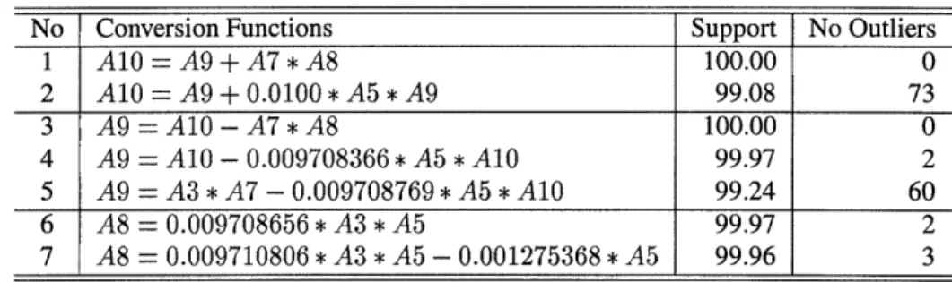
Finally, we included all the numerical attributes from the three databases in the mining process. We obtained the results as shown in Table 14.
Table 14: Results obtained when all attributes are included in mining process
No Conversion Functions Support No Outliers
1 A10 = A9 + A7 * A8 100.00 0 2 A10 = A9 + 0.0100 * A5 * A9 99.08 73 3 A9 = A10 - A7* A8 100.00 0 4 A9 = A10 - 0.009708366 * A5 * A10 99.97 2 5 A9 = A3 * A7 - 0.009708769 * A5 * A10 99.24 60 6 A8 = 0.009708656 * A3 * A5 99.97 2 7 A8 = 0.009710806 * A3 * A5 - 0.001275368 * A5 99.96 3
The functions with highest support for each attribute, i.e., Functions 1, 3 and 6 are selected as the conversion functions. It is not difficult to see that Functions 1 and 3 conform to the business rules. Function 6 is not that obvious as A8, the tax amount should be calculated from the sales, not A3 which is the total amount. However, we have A8 = (A3 - A8) * 0.01 * A5 Therefore 1 A8= · 0.01 A3 A5 1 + 0.01* A5 When A5 = 3, 0.01 A8 = 1-- * A3 * A5 = 0.009708656 * A3 * A5
which is the same as Function 6. When A5 = 0, A8 = 0, and Function 6 still holds. Because the original data only has two tax rates and one of which is zero, Function 6 can be obtained without partitioning the data. Again, there are two outliers because the tax amount in the two tuples shown in Table 13 is not correctly calculated based on the regulations.
5.5 Discussion
From the experimental results of the real world data set, we have some very interesting observations.
1. According to the systems from which the sales data were collected, the attribute values are calculated as follows:
* The amount of item lines is added together to obtain the sales amount of an invoice in the original currency, i.e., the currency in which the invoice was issued. Note that this amount does not appear in our data set as an attribute.
* From the sales amount, the goods and sales tax is calculated and rounded to cents (0.01) (A8 in our data set).
* The total amount billed is calculated as the sum of sales and tax which is A3 in our data set.
* A9 (A10) is calculated by multiplying sales (total) amount with the exchange rate. The result is
rounded to cents.
The exchange rate used in the system has 6 digits after the decimal point. Therefore, the data values may contain rounding errors introduced during calculations. In addition to the rounding errors, the data set also contains two error entries. Under our classification, the data set contains both context dependent and context independent conflicts.
Our first conclusion is this: although the training data set contains noises (rounding errors) and both
context dependent and independent conflicts (two outliers), the system was still able to discover the correct conversion functions.
2. One interesting function discovered by the system but not selected (eventually) is Function 2 in Table 12. Note that, from the expression itself, it is derivable from the other correct functions: Since A8 is the amount of tax in the original currency, A9 is the amount of sales in the local currency, A7 is the exchange rate, and
A5 is the tax rate(percentage), we have
A9 A8 = - * 0.01* A5 A7 That is, A7 · A8 A9 = 0.01A5 for A5 0 When A4 - 1, A5 = 3, so we should have
A7 A8
A9 = 0 = 33.33333 * A7 * A8. 0.01 3
which is the same as Function 2. The function was discarded because of its low support (99.36%). It seems puzzling that a function that is derivable from the correct functions has such low support so that it should be discarded.
It turns out that this phenomenon can be explained. Since, the derivation process is purely mathematical, it does not take into any consideration how the original data value is computed. In the real data set, the tax amount stored has been rounded up to 0.01. The rounding error may get propagated and enlarged when Function 2 is used. If exchange rate is 1.00 (i.e., the invoice is in the local currency), the possible error of
A9 introduced by using Function 2 to compute the sales amount from the tax amount could be as large as
33.33333*0.005. This is much larger than the precision of A9 which is 0.005. To verify the reasoning, we modified the function into
A7·A8
A9 = 0 = 33.33333 A7 * roundup(A8)


![Table 2: Example relations Attr. No. Relation Name Value Range Al stock, stk_rpt scode [1, 500]](https://thumb-eu.123doks.com/thumbv2/123doknet/14747122.578589/16.924.203.724.121.313/table-example-relations-attr-relation-name-value-range.webp)