Calculation of climatic reference values and its use for automatic outlier detection in meteorological datasets

HAL Id: hal-00297446

https://hal.archives-ouvertes.fr/hal-00297446

Submitted on 7 Apr 2008

HAL is a multi-disciplinary open access

archive for the deposit and dissemination of

sci-entific research documents, whether they are

pub-lished or not. The documents may come from

teaching and research institutions in France or

abroad, or from public or private research centers.

L’archive ouverte pluridisciplinaire HAL, est

destinée au dépôt et à la diffusion de documents

scientifiques de niveau recherche, publiés ou non,

émanant des établissements d’enseignement et de

recherche français ou étrangers, des laboratoires

publics ou privés.

Calculation of climatic reference values and its use for

automatic outlier detection in meteorological datasets

B. Téllez, T. Cernocky, E. Terradellas

To cite this version:

B. Téllez, T. Cernocky, E. Terradellas. Calculation of climatic reference values and its use for

au-tomatic outlier detection in meteorological datasets. Advances in Science and Research, Copernicus

Publications, 2008, 2, pp.1-4. �hal-00297446�

Adv. Sci. Res., 2, 1–4, 2008 www.adv-sci-res.net/2/1/2008/

©Author(s) 2008. This work is distributed under the Creative Commons Attribution 3.0 License.

Advances in

Science and

Research

EMS

Annual

Meeting

and

8th

Eur

opean

Confer

ence

on

Applications

of

Meteor

olo

gy

2007

Calculation of climatic reference values and its use for

automatic outlier detection in meteorological datasets

B. T´ellez, T. Cernocky, and E. Terradellas

Instituto Nacional de Meteorolog´ıa, CMT de Catalu˜na, Spain

Received: 31 October 2007 – Revised: 22 January 2008 – Accepted: 25 January 2008 – Published: 7 April 2008

Abstract. The climatic reference values for monthly and annual average air temperature and total precipitation in Catalonia – northeast of Spain – are calculated using a combination of statistical methods and geostatistical techniques of interpolation. In order to estimate the uncertainty of the method, the initial dataset is split into two parts that are, respectively, used for estimation and validation. The resulting maps are then used in the automatic outlier detection in meteorological datasets.

1 Introduction

In climatology, as well as in geography, in biology or in other fields, it is necessary to have climatic reference values for a specific spot or region. Rather often, there is not a meteo-rological station in the area of interest. Moreover, there is not any guarantee that data supplied by the nearest station describe accurately enough its climatic conditions. There are numerous methods to build a map to represent the spatial dis-tribution of climatic parameters: deterministic, probabilistic or physical methods, artificial neural networks, etc. (Lam, 1983; Demyanov et al., 1998; Ninyerola et al., 2007).

On the other hand, studies including analysis of meteoro-logical data usually require a preliminary arduous and un-pleasant debugging of the original datasets in order to purge wrong values. Most times, this task has been carried out through the comparison of the dataset to analyse with others recorded at nearby stations. Nevertheless, the method is not straightforward, especially when it is applied to magnitudes with strong spatial variations. Such variations are usually more evident in areas with complex physiographic features.

The problem can be mitigated through the use of the dif-ference with the redif-ference value instead of the original value. In Sect. 3, the method used to obtain the spatial distribu-tion of the climatic magnitudes is described. Secdistribu-tion 4 refers the attempts to automatically identify possible outliers from the spatial distribution of differences between meteorological data and climatic reference values.

Correspondence to: B. T´ellez

(bea@inm.es)

2 Geographic framework and data

The geographic framework for the present study is Catalonia, which is located in the north-eastern corner of the Iberian Peninsula. It has a surface area of 31 895 km2 _{and a}

sig-nificant geographic diversity, from the Mediterranean Sea to peaks over 3000 m above sea level in the Pyrenees. The cli-matological dataset contains 1961–1990 averages of monthly data (INM, 2000) recorded at 144 thermometric and 302 plu-viometric stations. 15 thermometric and 55 pluplu-viometric sta-tions are located over surrounding regions and have been in-cluded in the study in order to smooth border effects. Aux-iliary physiographic parameters, such as altitude, distance to sea or land slope have been retrieved from a digital elevation model (DEM) using GIS techniques. The DEM, with a 200-m resolution, has been provided by the Institut Cartogr`afic

de Catalunya (ICC).

3 Calculation of the climatic reference values

The climatic magnitudes – average monthly temperature and monthly precipitation – are represented using a combination of statistic methods and geostatistical techniques of interpo-lation. First, a multiple regression analysis yields a model that relates the climatic variable with several physiographic parameters. Then, the residuals, that is, the difference be-tween the observed values and the predictions of the linear model, are spatially interpolated using an ordinary kriging. The result, a map of residuals, shows the amount of vari-ability that is not explained by the regression model. This variability can be attributed either to errors in the original datasets or to relationships with physiographic or meteo-rological magnitudes that have not been considered in the

2 B. T´ellez et al.: Calculation of climatic reference values and its use for automatic outlier detection

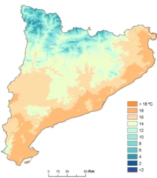
Figure 1.Reference values for the average temperature in October.

regression model. The final result is the addition of the map drawn from the model predictions and the map of residuals (see in Fig. 1 the final map of average temperatures in Octo-ber).

The physiographic parameters used in the regression are: altitude, latitude, longitude, distance to sea and average and minimum altitudes in circles of 5 to 40 km radius, which are considered, following Dyras et al. (2005), in order to account for topography at different scales. Then, the best predictive parameters for a given variable are chosen using a technique called stepwise regression (Hocking, 1976).

For average monthly temperature, altitude and distance to sea turn out to be the best predictive physiographic variables. The altitude explains most of the variance and it is significant in all cases. On the other hand, the distance to sea is only significant during the cold season, from October to March. The coefficients of the regression equation are displayed in Table 1.

For total monthly precipitation, the best predictive vari-ables are those related to altitude. Between May and Septem-ber, the average altitude in a 40-km radius circle explains most of the variance. In the other months, the most signif-icant variables are average and/or minimum altitudes for a 10/15-km radius circle. Latitude and longitude have also re-sulted to be significant in some cases. The coefficients of the regression equation are shown in Table 2.

An ordinary kriging is used to interpolate both temperature and precipitation residuals. The empirical semivariogram, built following Journel and Huijbreghts (1978), is modelled with an exponential curve, with the range set to 40 km. The values of nugget for the different months are in the range

Figure 2. Distribution of the thermal anomaly, that is, the differ-ence between the monthly-averaged temperature and its referdiffer-ence value, in June 2007. In both sides, zoom into areas where the slope exceeds the threshold value of 0.7◦_{C km}−1_.

0.2–1◦_C2 _{and 5–30 mm}2_{, and those of total sill in the range}

0.8–1.6◦_C2_{and 70–140 mm}2_.

The initial meteorological dataset is split into two parts in order to estimate the uncertainty of the method. The full pro-cess is first carried out using 70% of the initial data, which are selected at random. Then, the remaining 30% of data are compared with values retrieved from the resulting maps. This linear regression yields adjusted coefficients of deter-mination that are over 0.80 for average temperature (they range from 0.81 in July to 0.89 in November) and over 0.75 for total precipitation (they range from 0.75 in September to 0.90 in July). The highest errors are found in areas of great orographic complexity and sparse observational cover-age, where both the data fitting into the regression model and the interpolation of residuals are deficient. Anyway, since the overall results are acceptable, the process is finally car-ried out using the whole meteorological dataset.

4 Application of the reference values in debugging meteorological datasets

At the Instituto Nacional de Meteorolog´ıa, it has been im-plemented a method to automatically detect possible errors in the monthly average temperature and total precipitation datasets. It is based on GIS techniques and makes use of the climatic reference values previously computed.

The first step of the method is the calculation of the so-called monthly anomalies. The thermal anomalies are de-fined as the difference between a monthly averaged tempera-ture and its reference value. The precipitation anomalies are defined in a similar way, but they are expressed as a percent of the reference value.

Then, two different filters are applied in order to find out those stations whose data are suspicious and require fur-ther investigation. The first filter simply detects the stations

Table 1.Coefficients of the regression equation for monthly average temperature (T ): T =C+Ax1+Bx2, where x1is the altitude of the station,

x2is the distance to sea. The adjusted coefficient of regression and the root mean square error are also displayed.

C (◦_{C) A (}◦_{C/km) B (}◦_{C/km) Adj. r}2 _{R.M.S.E. (}◦_C) Jan 7.97 −2.9886 −0.0223 0.78 1.35 Feb 9.56 −4.6524 −0.0132 0.87 1.10 Mar 11.71 −5.4209 −0.0057 0.89 1.00 Apr 14.10 −6.2638 0.89 1.00 May 17.88 −6.0909 0.88 1.04 Jun 22.02 −6.1843 0.86 1.18 Jul 25.21 −6.8277 0.83 1.30 Aug 24.97 −6.3076 0.87 1.16 Sep 22.08 −6.1143 0.88 1.07 Oct 17.48 −5.0825 −0.0099 0.89 1.02 Nov 11.84 −3.7142 −0.0176 0.82 1.20 Dec 8.53 −2.8485 −0.0238 0.77 1.39

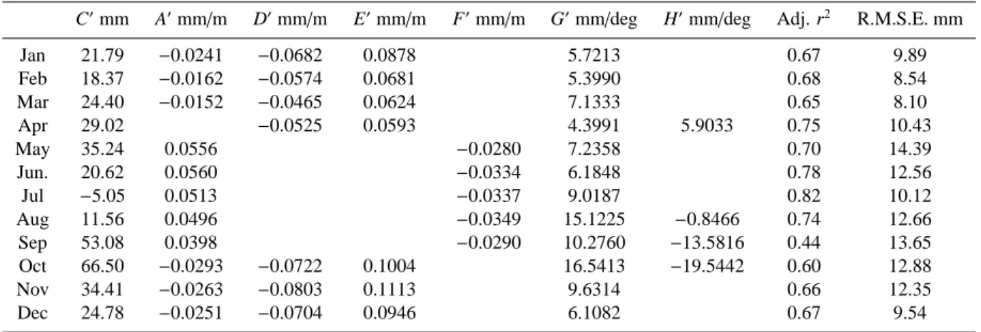
Table 2. Coefficients of the regression equation for monthly precipitation (P): P=C+A′_x

1+D′x2+E′x3+F′x4+G′x5+H′x6, where x1is the

altitude of the station (retrieved from the DEM), x2is the difference between the altitude of the station and the average altitude in a circle

of a 10 km-radius around it, x3is the difference between the altitude of the station and the minimum altitude in a circle of a 15 km-radius

around it, x4is the difference between the altitude of the station and the average altitude in a circle of 40 km-radius around it, x5is the eastern

longitude of the station and x6is the northern latitude (minus 40 degrees). The adjusted coefficient of regression and the root mean square

error are also displayed.

C′_{mm A}′_{mm/m D}′_{mm/m E}′_{mm/m F}′_{mm/m G}′_{mm/deg H}′_{mm/deg Adj. r}2 _{R.M.S.E. mm}

Jan 21.79 −0.0241 −0.0682 0.0878 5.7213 0.67 9.89 Feb 18.37 −0.0162 −0.0574 0.0681 5.3990 0.68 8.54 Mar 24.40 −0.0152 −0.0465 0.0624 7.1333 0.65 8.10 Apr 29.02 −0.0525 0.0593 4.3991 5.9033 0.75 10.43 May 35.24 0.0556 −0.0280 7.2358 0.70 14.39 Jun. 20.62 0.0560 −0.0334 6.1848 0.78 12.56 Jul −5.05 0.0513 −0.0337 9.0187 0.82 10.12 Aug 11.56 0.0496 −0.0349 15.1225 −0.8466 0.74 12.66 Sep 53.08 0.0398 −0.0290 10.2760 −13.5816 0.44 13.65 Oct 66.50 −0.0293 −0.0722 0.1004 16.5413 −19.5442 0.60 12.88 Nov 34.41 −0.0263 −0.0803 0.1113 9.6314 0.66 12.35 Dec 24.78 −0.0251 −0.0704 0.0946 6.1082 0.67 9.54

whose anomalies exceed a predefined threshold, which is specific for every variable. The second filter is a little more complex, since it detects groups of nearby stations with in-compatible data. The presence of areas with sharp spatial variations of anomalies is supposed to be related with the ex-istence of incompatible data.

To analyse the spatial variations of anomalies, they are first interpolated to 400-m spaced grid-points using an inverse-distance weighting method that avoids excessive smoothing. Then, the slopes in this grid are calculated and the second filter may detect the areas with the steepest slopes. The thresholds for suspicious values have been initially set to 0.7◦_{C km}−1_{for thermal anomalies and 7 km}−1_{for anomalies}

in precipitation, although they can be changed according to the particular data distribution.

Figure 2 illustrates the application of the method to monthly averaged temperatures recorded in June 2007. It shows a zoom into the areas where the slope in the distribu-tion of thermal anomalies exceeds the above-defined thresh-old. Further investigation revealed the presence of a wrong value in both areas.

5 Conclusions

A reliable map of climatic reference values allows precise es-timations of the represented climatic magnitudes in any area, even if there is not a meteorological station in it. It also may refer meteorological data gathered in a station to its corre-sponding climatic value, even if there is not a long and ho-mogeneous time series of such data in the station.

4 B. T´ellez et al.: Calculation of climatic reference values and its use for automatic outlier detection It has been implemented a method to automatically

de-tect possible errors in meteorological datasets. It performs very well for monthly precipitation in months with a smooth spatial distribution of anomalies. Sharper spatial distribu-tions of anomalies (occurrence of heavy local showers) lead to higher false alarm rates. The method also presents a good performance for average monthly temperature. Nevertheless, it is expected to improve the method skill through its sepa-rated application to monthly averaged minimum and maxi-mum daily temperatures.

Edited by: M. Dolinar

Reviewed by: L. de Salas, J. A. Fernandez, and another anonymous referee

References

Demyanov, V., Kanevsky, M., Chernov, S., Savelieva, E., and Timo-nin, V.: Neural network residual kriging application for climatic data, J. Geogr. Inform. Decis. Anal., 2, 215–232, 1998. Dobesch, H., Dumolard, P., and Dyras, I. (Eds.): Spatial

Interpola-tion for Climate data, Iste Publishing Co., 2007

Dyras, I., Dobesch, H., Grueter, E., Perdigao, A., and Tveito, O.: The use of Geographic Information Systems in climatology and meteorology: COST 719, Meteorol. Appl., 12, 1–5, 2005 Hocking, R. R.: The Analysis and Selection of Variables in Linear

Regression, Biometrics, 32, 1–51, 1976.

Instituto Nacional de Meteorolog´ıa: Valores normales de precip-itaci´on y temperatura de la Red Climatol´ogica (1961–1990), Se-rie Monograf´ıas, INM, Madrid, 2000.

Journel, A. G. and Huijbregts, C. J.: Mining Geostatistics, Aca-demic Press, London, 601 pp., 1978.

Lam, N. S.: Spatial interpolation methods: A review, Amer. Cart., 10, 129–149, 1993.

Ninyerola, M., Pons, X., and Roure, J. M.,: Objective air tempera-ture mapping for the Iberian Peninsula using spatial interpolation and GIS, Int. J. Climatol., 27, 1231–1242, 2007