Dynamic dependence analysis : modeling and inference of changing dependence among multiple time-series

(1)

Dynamic Dependence Analysis

:

Modeling and Inference of

Changing Dependence Among Multiple Time-Series

by

Michael Richard Siracusa

Submitted to the Department of Electrical Engineering and Computer Science in partial fulfillment of the requirements for the degree of

Doctor of Philosophy in

Electrical Engineering and Computer Science at the Massachusetts Institute of Technology

June 2009

©

MASSACHUSETTS INSTnTUTE OF TECHNOLOGY

AUG 0 7

2009

LIBRARIES

Dynamic Dependence Analysis

:

Modeling and Inference of

Changing Dependence Among Multiple Time-Series

by Michael Richard Siracusa

Submitted to the Department of Electrical Engineering and Computer Science on May 12, 2009

in Partial Fulfillment of the Requirements for the Degree

of Doctor of Philosophy in Electrical Engineering and Computer Science

Abstract

In this dissertation we investigate the problem of reasoning over evolving structures which describe the dependence among multiple, possibly vector-valued, time-series. Such problems arise naturally in variety of settings. Consider the problem of object interaction analysis. Given tracks of multiple moving objects one may wish to describe if and how these objects are interacting over time. Alternatively, consider a scenario in which one observes multiple video streams representing participants in a conversation. Given a single audio stream, one may wish to determine with which video stream the audio stream is associated as a means of indicating who is speaking at any point in time. Both of these problems can be cast as inference over dependence structures.

In the absence of training data, such reasoning is challenging for several reasons. If one is solely interested in the structure of dependence as described by a graphical model, there is the question of how to account for unknown parameters. Additionally, the set of possible structures is generally super-exponential in the number of time series. Furthermore, if one wishes to reason about structure which varies over time, the number of structural sequences grows exponentially with the length of time being analyzed.

We present tractable methods for reasoning in such scenarios. We consider two ap-proaches for reasoning over structure while treating the unknown parameters as nuisance variables. First, we develop a generalized likelihood approach in which point estimates of parameters are used in place of the unknown quantities. We explore this approach in scenarios in which one considers a small enumerated set of specified structures. Sec-ond, we develop a Bayesian approach and present a conjugate prior on the parameters and structure of a model describing the dependence among time-series. This allows for Bayesian reasoning over structure while integrating over parameters. The modular nature of the prior we define allows one to reason over a super-exponential number of structures in exponential-time in general. Furthermore, by imposing simple local or

(4)

plexity to polynomial-time complexity while still reasoning over a super-exponential number of candidate structures.

We cast the problem of reasoning over temporally evolving structures as inference over a latent state sequence which indexes structure over time in a dynamic Bayesian network. This model allows one to utilize standard algorithms such as Expectation Maximization, Viterbi decoding, forward-backward messaging and Gibbs sampling in order to efficiently reasoning over an exponential number of structural sequences. We demonstrate the utility of our methodology on two tasks: audio-visual association and moving object interaction analysis. We achieve state-of-the-art performance on a stan-dard audio-visual dataset and show how our model allows one to tractably make exact probabilistic statements about interactions among multiple moving objects.

Thesis Supervisor: John W. Fisher III

(5)

Acknowledgments

I would like to thank my advisor, John Fisher, for many years of guidance, encourage-ment and generous support. I met John during my first visit to MIT and find it difficult to imagine getting through graduate school without him. His dedication to research, his willingness to dive into the details and his humor not only made him a perfect advisor, but also a great friend.

I would also like to thank Alan Willsky and Bill Freeman for their insight and advice while serving on my thesis committee. I was welcomed into Alan's research group shortly after my Masters and have greatly appreciated our weekly grouplet discussions. It always amazes me how all those ideas and information is stored in one man's brain. Talking with Bill or even passing him in a hallway always brings a smile to my face and reminds me how fun and exciting good research is.

I would also like to thank Alex Ihler, Kinh Tieu, Kevin Wilson, Biswajit Bose, Wanmei Ou and Emily Fox for always being willing to help, listen, and discuss research ideas. Archana Venkataraman and Kevin Wilson get a special thank you for getting through early drafts of this dissertation and coming back with great comments and improvements.

I have been fortunate to have had the opportunity to interact with some the most intelligent and unique people I know while at the Computer Science and Artificial Intelligence Laboratory and in the Stochastic Systems Group. I have learned so much from them and have come away with so many great friendships. I could not adequately thank them all here.

Most importantly, I would like to thank my family. All my successes would have been empty and road blocks insurmountable without their patience, love and encouragement. I especially would like to thank my nephews Simon, Ethan, Alex and Adam and my niece Cate for reminding me of what is important. Finally, I'd like to thank my sweet Ana for giving me a reason to finish and look towards the future.

(6)

Different aspects of this thesis was supported by the Army Research office under the Het-erogenous Sensor Networks MURI, the Air Force Office of Scientific Research under the In-tegrated Fusion, Performance Prediction, and Sensor Management for Automatic Target Ex-ploitation MURI, the Air Force Research Laboratory under the ATR Center, and the Intelligence Advanced Research Projects Activity (formerly ARDA) under the Video Analysis and Content Extraction project

(7)

Abstract Acknowledgments List of Figures List of Tables List of Algorithms 1 Introduction 1.1 Motivation 1.2 1.3 1.4 1.5 Objective . ... Our Approach ...

Key Challenges and Contributions Organization of this Dissertation

2 Background

2.1 Statistical Dependence ... 2.2 Graphical Models ...

2.2.1 Graphs ... 2.2.2 Factor Graphs ...

2.2.3 Undirected Graphical Models 2.2.4 Bayesian Networks ... 2.3 Time-series ...

2.4 Parameterization, Learning, Inference and Evidence

6.1.2 Illustrative Synthetic Example of Two Objects Interacting . . . . 6.2 Experiments . . . . ... 6.2.1 Static Interactions . .... -. -. -. -. -. -. -. -. -. -. -. -. -. -. -. -. -. -. -. -. 8 7 - -. 89 . 90 . 91 . 92 . 95 . 102 * 103 104 107 * 109 111 112 112 .113 114 115 116 116 117 118 120 120 122 123 124 135 137 138 139 140 142 142

(10)

6.2.2 Dynamic Interactions ... Follow the Leader . . ... Basketball...

6.3 Summary . . . ...

7 Conclusion

7.1 Summary of Contributions ... 7.2 Suggestions for Future Research ...

7.2.1 Alternative Approaches to Inference . . . . 7.2.2 Online Dynamic Dependence Analysis . . . . 7.2.3 Learning Representation and Data Association . 7.2.4 Latent Group Dependence . ...

7.2.5 Locally Changing Structures . ...

7.2.6 Long Range Temporal Dependence . . . .. 7.2.7 Final Thoughts . . ...

A Directed Structures

A.1 Sampling Structure . . ...

A.1.1 Sampling Without Global Constraints . . . . A.1.2 Sampling Directed Trees and Forests . . . . A.2 Sampling Parameters . . ...

A.3 Obtaining the MAP Structure ... A.3.1 Directed Trees and Forest ... A.4 Notes on Numerical Precision ...

B Derivations

B.1 Derivation of Equations 3.38 and 3.40 . ...

B.2 Consistent ML Estimates: Equations 3.42 through 3.45

... . 144 ... . 144 . . . ... 149 ... . 152 155 155 156 157 157 158 158 159 160 1i61 163 163 163 164 166 169 170 173 175 . . . . 175 . . . . 178 . . . . 180 181

B.3 Derivation of Expectations of Additive Functions over Structure B.4 Derivation of Equations 4.20 and 4.21 . ... ...

(11)

(12)

(13)

List of Figures

Dependence .. . . ...

Equivalent Graphical Models . ... Markov Models for Time-Series ... Deterministic vs Random Parameters . ... Example Dirichlet Distributions . ...

Examples of the Normal-Inverse-Wishart distribution . . .

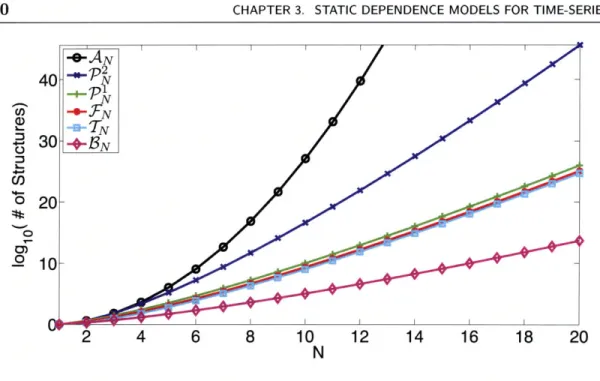
Three Abstract Views of a Static Dependence Model . . . Example FactM(1) Structure and Association Graph . . . Example TIM(1) Model Structure and Interaction Graph The Size of Sets of Directed Structure vs N ...

.. . . . . 29 .. . . . . 31 .. . . . . 34 .. . . . . 35 .. . . . . 39 . . . . . 41 . 51 . 55 . . 66 70 First Order Dynamic Dependence Model . . . . . . . . .. A Sample Draw from an HFactMM(0,2) . . . . . . . . .. 2D Gaussian Experimental Results Using a Windowed Approach . . 2D Gaussian Experimental results Using an HFactMM and FactMM A More Complex 2D Example .. ... ...

Quantization

of Each Observed Time-Series D . . . . . . . ... A STIM(0,K) shown as a directed Bayesian network . . . . 2.1 2.2 2.3 2.4 2.5 2.6 3.1 3.2 3.3 3.4 4.1 4.2 4.3 4.4 4.5 4.6 4.7 5.1 5.2 5.3 5.4 5.5 5.6 88 97 98 98 101 102 103 . . . . . . 113 . . . . . . 114 . . . . . 115 . . . . . 117 . . . . . 118 . . . 119 The CUAVE Dataset . . ...

"Look Who's Talking" Data ... NIST Data ... ...

Video and Audio Feature Extraction Block Diagrams .. Sub-blocks for Audio and Video Processing . . . . The Three Audio and Video Factorizations Considered .

(14)

5.7 Results for CUAVE Sequence g09 ... ... 121

5.8 Results for the "Look Who's Talking" Data . ... ... 124

5.9 Results for NIST data ... ... 125

5.10 Dependence Analysis for CUAVE Sequence g09 . ... 127

5.11 Dependence Analysis for the "Look Who's Talking" Sequence ... 128

5.12 Dependence Analysis for the NIST Sequence . ... 129

5.13 Analysis of State Distinguishability . ... .. 130

5.14 Stationarity Analysis for CUAVE Sequence g09 . ... 132

5.15 Stationarity Analysis for the "Look Who's Talking" Sequence ... 133

5.16 Stationarity Analysis for the NIST Sequence . ... 134

6.1 Interaction Graphs for Two Objects ... . 138

6.2 The Average Edge Posterior for Different p and

#

of samples T ... 142

6.3 A screenshot from our "Interaction Game" ... 143

6.4 Resulting Posterior Interaction Graphs for Specific Behaviors ... 145

6.5 Samples of z Using a STIM(1,3) on the Follow the Leader Dataset . . . 116

6.6 Highest Log Likelihood Sample for Follow the Leader Data ... 148

6.7 Typical Sample for Follow The Leader Data . ... 148

6.8 Sample Drawn using a STIM(1,6) on the Follow the Leader Data . . . . 149

6.9 Sample Frame from Basketball Data . ... . 150

6.10 Sampled State Sequence for the Basketball Data . ... 151

6.11 Influence of Point Guard A (PG A) ... .. 153

7.1 Latent Group Dependence ... ... 158 7.2 Graph Models for the Proposed Local Dependence Switching ... 1.60

(15)

List of Tables

3.1 Notation Summary ... . . ... 49

3.2 Example FactMs . ... ... 54

5.1 Results Summary for CUAVE ... ... 121

5.2 Full Results on CUAVE Group Dataset . ... 123

6.1 Basketball Results Showing Probability of Root . ... 151

(16)

(17)

List of Algorithms

3.4.1 Bayesian Inference of TIM Structure for Static Dependence Analysis . . 81

4.3.1 The EM Algorithm for a Dynamic Dependence Model . ... 93

4.3.2 The Forward-Backward Algorithm ... .. 94

4.4.1 The Three Main Steps a STIM Gibbs Sampler. . ... 105

4.4.2 Step 1 of the STIM Gibbs Sampler During Iteration i . ... 106

4.4.3 Step 2 of the STIM Gibbs Sampler During Iteration i. ... . 106

4.4.4 Step 3 of the STIM Gibbs Sampler During Iteration i ... 106

A.1.lSampling E Without Global Constraints . ... 165

A.1.2The RandomTreeWithRoot Algorithm with Iteration Limit ... 167

A.1.3The RandomTreeWithRoot Supporting Functions . ... 168

A.2.1Procedure for Sampling Parameters Given Structure . ... 168

A.3.10btaining MAP E without Global Constraints . ... 169

A.3.2The Chu-Liu, Edmonds, Bock Algorithm . ... .. . . 171

(18)

(19)

Chapter 1 Introduction

In this dissertation we investigate the problem of analyzing the statistical dependence among multiple time-series. The problem is cast in terms of inference over structure used by a probabilistic model describing the evolution of these time-series, such as an undirected graphical model or directed Bayesian Network. We are primarily concerned with the structure of dependence described by the presence or absence of edges in a graphical model and as such we treat model parameters as nuisance variables. Building upon the large body of work on structure learning and dynamic Bayesian networks we present a model which yields tractable inference of statistical dependence relationships which change over time. We demonstrate the utility of our method on audio-visual association and object-interaction analysis tasks.

* 1.1 Motivation

When designing and building intelligent systems it would be beneficial to give them the ability to combine multiple sources of sensory information for the purpose of interpreting and understanding the environment in which they operate. Fusion of multiple sources of disparate information enables systems to operate more robustly and naturally. One inspirational example of such a system is the human being. Our five basic sensing modalities of sight, hearing, touch, taste and smell are combined to provide a view of our environment that is richer than using any single sense in isolation. In addition to being inherently multi-modal, human perception takes advantages of multiple sources of information within a single modality. We have two eyes, two ears and multiple pathways for our sense of touch. Moving beyond the act of sensing, the human brain is highly effective at extracting, combining and interpreting higher-level information from these sources. For example, using our visual input we are able to track multiple moving

(20)

objects and combine this information with what we hear in order to help identify the source of a sound.

There are two main challenges when designing systems that fuse information from multiple time-series. The first challenge is choosing how to represent the incoming data. The high dimensional nature of each data source makes processing the raw sensory input computationally burdensome. Extracting features from each data source can alleviate this problem by eliminating information that is irrelevant or inherently noisy. For example, computation could be reduced if one were able to extract the location of multiple objects in a scene to analyze their behaviors rather than processing the entire visual scene as a whole. Even if dimensionality is low or features are extracted, the important question of determine which features are informative for the specific task remains. There has been considerable work on the task of general feature selection [41, 8, 53, 55] and on learning informative representations across multiple data sources [29, 84, 30]. This dissertation will assume the challenge of representation has been addressed by one of these existing approaches or by carefully hand picking features which are sufficiently informative for the application of interest.

The second challenge is that of integration. Once features are extracted the there is a question of how information obtained from them can be effectively combined. Sim-ple strategies can be devised assuming the data sources are independent of each other. While computationally simple, such strategies neglect to take advantage of any shared information among the inputs. The opposite extreme is to consider all possible relation-ships among the inputs. This comes at the cost of a more complex model for integration. Thus, a key task for fusing information among multiple data sources is to identify the relationships among them. If one knew that the dependence among the data sources this knowledge could be exploited to perform efficient integration. This is the main focus of this dissertation: developing techniques for identifying the relationships among the multiple sources of information. In many tasks, identify these relationships is the main result one is interested in.

Consider a scene in which there are several individuals, each of whom may be speaking at any given moment. Assume a recording of the scene produces a single audio stream in addition to a wide angle video stream. For each individual in the scene a separate video stream representing a region of the input video can be extracted. Given this data over a long period of time, one useful task is to determine who, if anyone, is speaking at each point in time. Humans are very effective at this task. The solution to

(21)

Sec. 1.1. Motivation

this audio-visual association problem has wide applicability to tasks such as automatic meeting transcription, social interaction analysis, and control of human-computer dialog systems. The semantic label identifying who is speaking can be related to associating the audio stream with many, one or none of the video streams. For example, the identification that "Victoria is speaking" indicates that the video stream for Victoria is associated with the audio stream.

Next, consider a scene with multiple moving objects. For example, think about a basketball game in which the moving objects are the players on each team and the ball. Given measurements of the position of these objects over a long duration of time, a question one may ask is: Which, if any, of these objects are interacting at each point in time? The answer to this question is useful for a variety of applications including anomalous event detection and automatic scene summarization. In this specific example of a basketball game, understanding the interactions among players can help one identify a particular play, which team is on offense, and who is covering whom. This is a common and natural task regularly performed by humans. Heider and Simmel [45] note that when presented a cartoon of simple shapes moving on a screen, one will tend to describe their behavior with terms such as "chasing", "following" or being independent of one another. These semantic labels describe the interaction between objects and allow humans to provide a compact description of what they are observing.

Underlying both of these problems is the task of identifying associations or inter-actions among the observed time-series. The words association and interaction both describe statistical dependence. When we say the audio stream is associated with video stream for Victoria, we are implying the two time-series share information and should not be modeled as being independent of one another. Similarly, when we claim two objects are interacting we are implying some statistical dependence between them. For example, a "following" interaction implies a causal dependence between the leader's current position and the follower's future position.

Note that with each of these dependence relationship there is the question of iden-tifying the nature of that dependence. There are many ways in which time-series can be dependent on each other. Associated with a particular dependence structure are a set of parameters describing that dependence. For example, these parameters will describe the tone of Victoria's voice in the audio stream and exactly how motion in the video stream is associated with changes in the audio. In the object interaction analysis scenario the parameters describing the causal dependence for a "following" behavior

(22)

will characterize how fast the objects are moving and how closely the leader is being followed. Our primary interest is in identifying the presence or absence of dependence rather than accurately characterizing the nature of that dependence describe by these parameters.

* 1.2 Objective

We develop a general framework for the task of dynamic dependence analysis. The primary input to a system performing dynamic dependence analysis is a finite set of discrete-time vector-valued time-series jointly sampled over a fixed period of time. The output of the system is a description of the statistical dependence among the time-series

at each point in time. This description may be in the form of a point estimate of or distribution over dependence structure. The techniques presented in this dissertation have additional inputs such as:

* The maximum number of possible dependence relationships the system should consider modeling the time-series changing among over time.

* A specified class of static dependence models that will be used to described a fixed dependence among the time-series.

* A prior on the dependence structures of interest and an optional prior on param-eters describing the nature of dependence.

* 1.3 Our Approach

Past approaches to the problem of audio-visual association have either been based on basic measures of dependence over fixed windows of time [46, 84, 30, 68] or on incorpo-rating training data to help classify correct speaker association [68, 72]. Similarly, past approaches for object interaction analysis have relied on measuring statistical depen-dence among small groups of objects assuming the interaction is not changing [88] or on trained classifiers to detect previously observed interacting behaviors [66, 49, 48, 69].

Building upon previous work we wish to address the issues that arise when per-forming dependence analysis on data in which the structure may change over time. Furthermore we wish to do so in the absence of large training datasets. Approaches that rely on general measures of statistical dependence are powerful in that they do not rely on any application specific knowledge and can be adapted easily to many other

(23)

Sec. 1.4. Key Challenges and Contributions 23

domains. Previous work has primarily focused on the use of windowed approaches [68, 72]. That is, given a window of time they measure dependence assuming it is static. By sliding this window over time such approaches attempt to capture changing dependence. When using such an approach the window size used must be long enough to get an accurate measure of dependence. At the same time it must be short enough as to not violate the assumption of a static dependence relationship being active within the window. That is, there is a tradeoff between window size and how fast dependence structures can change. Approaches that use training data have the advantage of being specialized to the domain of interest and may be able to overcome some of these issues by only needing a few samples to identify a particular structure. However, domain specific training data is not always available.

Our core idea is that rather than treating the problem as a series of windowed tasks of measuring static dependence, we cast the problem of dynamic dependence analysis in terms of inference on a dynamic dependence model. A dynamic dependence model explicitly describes dependence structure among time-series and how this dependence evolves over time. Using this class of models allows one to incorporate knowledge over all time when making a local decision about dependence relationships. Additionally, it allows one to take advantage of repeated dependence relationships from different points in time. We demonstrate the advantage of this approach over windowed analysis both theoretically and empirically.

* 1.4 Key Challenges and Contributions

This dissertation addresses a set of key challenges and makes the following contributions:

How does one map the associations in the audio-visual task and the interactions in the object interaction analysis task to a particular sta-tistical dependence structure?

We introduce two general static dependence models: a static factorization model (FactM) and temporal interaction model (TIM). The FactM describes multiple time-series as sets of independent groups. That is, it explicitly models how the distribution on time-series factorizes. In the audio-visual association task, reason-ing over associations between the audio and video streams is related to reasonreason-ing over factorizations.

(24)

The TIM allows one to provide more details about the dependence among time-series. The model takes the form of directed Bayesian network describing the causal relationships between the current value of a single time-series based on the finite set of past values of other associated time-series. We treat the problem of identify interactions as one of identifying the details of these causal relationships.

How many possible structures are there and is it tractable to consider all of them?

The number of possible dependence structures among N time-series is super-exponential in N, O(NN). For many applications, such as the audio-visual as-sociation task, there is a small number of specific structures one is interested in identifying and thus inference is generally tractable. However, in other applica-tions, one may want to consider all structures or significantly large subset that grows with N. We show that a super-exponential number of structures can be reasoned over in exponential-time in general by exploiting the temporal causality assumptions in our TIM. We further show that by imposing some simple restric-tions on the structures considered one can reason over a still super-exponential number of them in polynomial-time.

How does one incorporate prior knowledge about dependence?

In some applications we may have some prior knowledge about which dependence structures are more likely than others. When considering a tractable set of struc-tures a simple discrete prior distribution can be placed over them. However, this approach becomes intractable as the number of structures considered increases. Building upon the type of priors used for general structure learning [62, 54, 33] we present a conjugate prior on structures for a TIM which allows for efficient posterior updates.

When analyzing a large number of time-series, trying to uncover a single "true structure" active at any point in time is often less desirable than a full charac-terization of uncertainty. Using this class of priors we obtain a distribution over structure rather than a point estimate. In addition, the exact posterior marginal distributions and expectations can be obtained tractably. This allows for a de-tailed characterization of uncertainty in the statistical dependence relationships

(25)

Sec. 1.5. Organization of this Dissertation

How does one separate the task of identifying dependence structure from that of learning the associated parameters?

That is, an issue which arises when inferring dependence relationships is how to deal with unknown parameters which describe the nature of dependence. In this dissertation we will explore two approaches. We show how a maximum likelihood approach can be used to obtain a point estimate of the parameters from the data being analyzed. We show theoretically and empirically how this approach causes problems for windowed dependence analysis techniques while it can help our dynamic dependence approach. Alternatively, we present a conjugate prior over parameters of a TIM and show how to tractably perform exact Bayesian

inference integrating over all possible parameters.

How does one model dependence that may change over time?

Building on the large body of work on dynamic Bayesian networks (DBNs) and hidden Markov models (HMMs) we introduce a dynamic dependence model which contains a latent state variable that indexes structure. In this dissertation we assume the number of possible structures is known a priori. That is, the number of possible latent state values is assumed to be known. A simple Markov dynamic is placed on this latent variable to model how structure evolves over time. Adopting such a model allows one to infer changes in structure via the use of standard forward-backward message passing algorithms. This allows one to reason over an exponential number of possible sequence of dependence relationships in linear time.

Additionally, we formulate both audio-visual association and object interaction anal-ysis tasks as special cases of dynamic dependence analanal-ysis. We show how state-of-the-art

performance on a standard dataset for audio-visual speaker association can be achieved with our method. We demonstrate the utility of our approach in analyzing the

inter-actions among multiple moving players participating in a variety of games.

* 1.5 Organization of this Dissertation

We begin in Chapter 2 with a review of statistical dependence, graphical models, con-jugate priors and time-series models. This will give the background needed for the rest of the dissertation. Chapter 3 introduces our two static dependence models which

(26)

assumed a fixed dependence structure over all time. We discuss conjugate priors over structure and detail inference on such models in both a classical maximum likelihood and Bayesian framework. Chapter 4 extends these models to become dynamic depen-dence models by embedding them in hidden Markov model. We show theoretically how such models have a distinct advantage over windowed approaches for dynamic depen-dence analysis. Details are given for maximum likelihood inference using Expectation Maximization and Bayesian inference using a Gibbs sampling approach. Chapters 5

and 6 present experiments using our models in audio-visual association and objective interaction analysis tasks respectively. We conclude with a summary and discussion of

(27)

Chapter 2 Background

In the previous chapter we introduced the general problem of analyzing dependence relationships among multiple time-series. In this chapter we give a brief overview of the basic technical background the rest of the dissertation relies on. We use statistical models to describe time-series and the relationships among them. That is, we describe time-series in terms of random variables and their associated probability distributions. We assume the reader has a basic understanding of probability theory which can found in introductory chapter of a wide variety of standard textbooks (c.f. [5, 70]).

We begin by defining statistical dependence. This is followed by a review of graphical models and how they can be used to encode the structure of dependence relationships among a set of random variables. Next, in Section 2.3, we discuss time-series in terms of discrete-time stochastic processes and present the use of a simple Markov model for describing temporal dependence. In Section 2.4 we overview the standard parametric models which will be used in this dissertation along with a discussion of conjugacy, inference and learning. Lastly, we briefly present select topics from information theory and their relation to the problem of analyzing statistical dependence.

The intent of this chapter is to provide a brief overview of the selected material. We refer the reader to standard text books for a more rigorous treatment and proofs (c.f.

[5, 70, 21, 73]).

N

2.1 Statistical Dependence

We start by defining statistical dependence. Intuitively, two random variables are de-pendent if knowledge of one tells you something about the other. To formalize this abstract concept on can more concretely define statistical independence. Two random variables, x and y, are statistical independent if and only if their joint distribution is a

(28)

product of their marginal distributions:

p (x,y) = p(x)p(y). (2.1)

The notation x IL y is used to denote statistical independence. Using the fact that

p (x, y) = p (x) p (ylx) = p (y) p (xly) this requirement is equivalent to saying that the

conditional distribution of one random variable given the other is not a function of what is being conditioned on:

p (xly) = p (x) and (2.2)

p (yx) = p (y) . (2.3)

This definitions can be easily extended to more than two random variables. The joint of distribution of a collection of independent random variables factorizes as product of their marginals and all conditional distributions are independent of the random variables conditioned on.

A simple example of statistical independence is when x and y are the results of coin tosses of two separate coins. Each coin may have its own bias / probability of heads versus tails, but if they are two physically separate coins tossed in isolation, knowledge of whether x is heads or tails tells you nothing about the outcome y.

Statistical dependence is simply defined to be the absence of statistical indepen-dence. That is, two random variables are dependent if their joint distribution is not the product of their marginal distributions. Going back to a simple coin example, let x be the result of a fair coin toss such that p (x = heads) = p (x = tails) = .5. Given x, imagine placing a small weight on a second fair coin so that it is biased to be more likely to land on the same side as x. Let y be the result of flipping this biased coin. To be concrete, assume this bias favors x with probability .9, p (y = headslx = heads) =

p (y = tailslx = tails) = .9 and p (y = tails x = heads) = p (y = tailslx = heads) = .1. Here, x and y are statistically dependent. Our description of the experiment clearly indicates how knowledge of x tells us something about y. Using Bayes' rule it is easy to show that the reverse is also true and knowledge of y also tells us something about x. Specifically, p (x = headsly = heads) = .9 * .5/(.9 * .5 + .1 * .5) = .9 while

p (x = headsly = tails) = .1.

Another important concept is that of conditional independence. Two random vari-ables x and y are conditionally independent given another random variable z, x II y I z, if and only if:

(29)

Sec. 2.2. Graphical Models 29

Independent Dependent

P (Xl)p (X2) p (Xl, X2)

Figure 2.1. Dependence: Undirected graphical models depicting independent and dependent distri-butions for two random variables.

or equivalently

p (xly, z) = p (xlz) and (2.5)

p (ylx, z) - p (yz) (2.6)

It is important to note that conditional independence does not imply independence and vice versa. We will give some specific examples in the following section when discussing Bayesian networks.

N

2.2 Graphical Models

In the previous section we discussed the link between statistical independence of ran-dom variables and the structure of their joint distribution. Probabilistic graphical models combine the syntax of graph theory with probabilistic semantics to describe the dependence structure among a set of random variables. Graphs are used to de-scribed the overall joint probability of the random variables in terms of local functions on subgraphs. This local decomposition allows for efficient reasoning over the random variables represented. More importantly for this dissertation, graphical models provide a convenient way to specify and understand conditional independence relationships in terms of graph topology. For example, consider the two undirected graphical models depicted in Figure 2.1. It is intuitive and simple to read dependence information from these graphs.

In the following section we review basic graph theory to establish some notation. We then discuss different classes of graphical models, each of which uses a different graphical representation to described conditional independence. Again, these sections provide a quick overview and we refer the reader to standard text books for a more detailed treatment [73].

(30)

U 2.2.1 Graphs

A graph G = {V, E} is a set of vertices/nodes V and a collection of edges E. Edges

(i,

j)

E E connect two different nodes i,j E V. Edges can be either undirected or

directed. In undirected graphs, the edge (i,

j)

is in E if and only if (j, i) is as well. A vertex

j

is a neighbor of vertex i if (i, j) E E and the set neighbors for vertex i is simply the collection of all such j E V. A path is defined as a sequence of neighboring nodes. If there is a path between all vertices the graph is said to be connected. For undirected graphs a clique C C V is a collection of vertices for which all pairs are have an edge between them. If the entire graph forms a clique the graph is said to be complete.

In a directed graph, directed edges (i,

j)

connect a parent node i to its child

j.

Throughout the dissertation we will use the notation E to represent a set of directed edges and will represent them as arrows in figures. For example, see Figure 2.2(b). The set of all parents pa (i, E) for a particular node i is the set of all

j

E V such that

(i, j) E E. For brevity we will often drop the E and refer to this set as pa (i).

A useful generalization of a graph is a hypergraph. A hypergraph H = {V, F} is composed of vertices V and associated hyperedges F. Each hyperedge f E F is specified by any non-empty subset of V. That is, each hyperedge can connected one or more vertices. Two vertices are neighbors in this hypergraph if they belong to a common hyperedge. We represent a hypergraph as a graph with extra square nodes for each hyperedge. All vertices which belong to that hyperedge are connected to the associated square node. This makes the graph bipartite in that edges only occur between vertices and the square hyperedge nodes. See Figure 2.2(c) for an example.

* 2.2.2 Factor Graphs

Factor graphs are a class of graphical models which use a hypergraph H to specify the

form of the joint probability distribution on a set of random variables [58]. Let xv represent the set of all random variables {xili E V}. Given a set of hyperedges F, a factor graph represents the joint distribution p (xv) as

p(xv) = I H / f(xf), (2.7)

fEF

(31)

Sec. 2.2. Graphical Models 31

X1

X2

X1

X2

X1

X

2

X1

X2

X3X3

X3

X4

(a) (b) (c) (d)

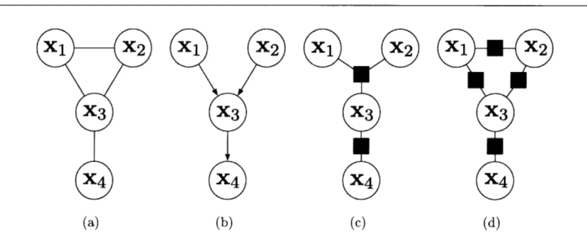
Figure 2.2. Equivalent Graphical Models: Three graphical models using different representations to describe the joint distribution of four random variables. (a) A markov random field (b) a directed Bayesian network. (c) a factor graph. (d) a second factor graph with the same neighbor relationships

the partition function, guarantees proper normalization. That is,

Z = Z I-bf(xf)

(2.8)

xV feF

Figure 2.2(c) shows an example in which 1

P (X₁, X2, X3, X4) = )1,2,3(X1, X2, X3))3,4 (X3, X4). (2.9)

In the equation above, and in general, of(xf) does not correspond to the marginal distribution p (xf). However, in this dissertation we will use factor graphs in situations in which each random variable belongs to a single hyper edge and the

4

functions correspond to marginal distributions.

Conditional independence information can be read directly from a factor graph. Any two random variables xi and xj are conditional independent given a set xZ for

Z C V if every path between xi and xj in the hypergraph passes through some vertex

k E Z. Two random variables are marginally independent if there is no path between

them. In Figure 2.2(c), x4 IL x1 I x3. Using this fact it is simply to see that xi is independent of all other random variables given its neighbors in the factor graph.

* 2.2.3 Undirected Graphical Models

Undirected graphical models, generally referred to as Markov Random Fields (MRFs), encode conditional independence relationships in a graph G = {V, E}. Closely related to

(32)

factor graphs, MRFs represent the joint distribution as a product of potential functions

on cliques c:

p(xv) = 0 c(xc) (2.10)

C

where, again, Z is the normalization constant. MRFs have the same conditional in-dependence properties as factor graphs in that two random variables x_iand xj are conditionally independent given a set of random variables that must be passed through for every path between x_iand x .

Figure 2.2(a) shows an MRF with the same conditional dependence relationships as the factor graph in Figure 2.2(c). In fact, in general, there are many factor graphs which represent the same conditional independence relationships for a given MRF. Figure 2.2(d) shows a second factor graph which has the same dependence properties as Figure 2.2(a). Factor graphs have more flexibility in that they can explicitly specify how potentials on cliques factor, further constraining the space of possible joint distributions represented. This flexibility comes from their more general hypergraph specification.

* 2.2.4 Bayesian Networks

Bayesian networks are graphical models which can encode causality via a directed

rep-resentation. Given a directed graph G = {V, E} a Bayesian network represents a joint probability which factors as a product of conditional distributions:

p(xv) H= p (Xi Ipa(i) . (2.11)

iEV

If a node has no parents, pa (i) =

0,

the we define p (xi/x0) = p (xi). This factorization is only valid when E is acyclic. That is, it represents a graph in which there is no directed path from one node back to itself. Figure 2.2(b) depicts a Bayesian network with:

p (, X2, X3, X4) = p(X1)p(

(X

2)p(X3 X1, X2)p(X4 X3) (2.12)

This decomposition exposes an underlying generative process.

Reading conditional independence from a Bayesian network is more complicated than for undirected models and factor graphs. The Bayes Ball algorithm provides a way of extracting independence relationships from Bayesian network structure [79].

(33)

Sec. 2.3. Time-series

on its parents, its children, and its children's parents. A Bayesian network can be

moralized into an MRF by connecting the parents of each node with an undirected

edge and replacing all directed edges with undirected ones. Figure 2.2(a) is a moralized version of Figure 2.2(b).

Bayesian networks can explicitly represent certain statistical dependence relation-ships factor graphs and MRFs cannot. For example, consider the V structure found between xl,x3 and x3 in 2.2(b). A classic example with this dependence structure is a scenario when x, and x2 represent the outcomes of two independent coin tosses. Let

x3 be an indicator of whether x, and x2 had the same outcome. Causally x, and x2 are independent, x1 _L x2, but conditioning on knowing x3 they become dependent. Knowing whether the coin tosses where the same or not and the outcome of x1 tells you a lot about x2. In order to capture this relationship in an MRF, the three random vari-ables must form a clique (adding an edge between x, and x2). This is a case in which independence does not imply conditional independence. The reverse is true for x, and

x4 in Figure 2.2(b). They are statistical dependent but are conditionally independent given x3, x1 IL X41 X3.

* 2.3 Time-series

So far in this chapter we have been talking about statistical dependence among, and distributions for, general sets of random variables. In this dissertation we a interested in the dependence among time-series. A time-series can be modeled as a discrete time

stochastic process whose value at time t is represented by a random variable, x_t. A

stochastic process is fully characterized by all joint distributions of the process at dif-ferent points in time. A discrete stochastic process over a finite interval from 1 to T is completely specified in terms of its joint p (x1, x2,... , XT). We will often use the nota-tion X1:T to denote such a sequence. If T is not fixed, this distribution would have to be specified for all possible T one expects to encounter. Such an approach is not tractable, and thus it is common to make certain assumptions about the temporal dependence.

One simple model for time-series is to consider each time point to be independent and identically distributed (i.i.d.) such that:

T

P (XI:T) = p (xt) (2.13)

t=1

(34)

(a) First order (b) Second order

Figure 2.3. Markov Models for Time-Series: Directed Bayesian network (DBN) (a) represents a first order model and DBN (b) represents a second order model.

the past can help predict future time-series values. A Markov model is another tractable model which can capture some of this dependence. Consider the fact that the full joint distribution can always be factorized as

T

p (X1:T) = p

(xt

X1:t-1)

(2.14)

t=1

An r-th order Markov model is obtained if one assume the right-hand side is only dependent on the previous r time points. A first order model is simply

T

P (Xl:T) = p (x1)

fp

(xtlxt_1). (2.15) t=2

and is depicted as a directed Bayesian network in Figure 2.3(a). A second order model is shown in Figure 2.3(b). Note that a zero order model is simply i.i.d.

We will use this class of models for our time-series throughout the dissertation. Note, here we are describing a single time-series X1:T. In Chapter 3 we will discuss models for jointly describing multiple time-series in which the temporal dependence is fixed but the dependence across time-series is unknown.

* 2.4 Parameterization, Learning, Inference and Evidence

In the previous sections we discussed statistical dependence and how it can be encoded by a graphical model. We discussed how these models specify the form of the joint distribution in terms of local conditional probability distributions or potential func-tions. Implicitly each of these local distributions and potential functions has a set of parameters associated with it. The parameters fully specify its form. So far, we have been hiding these parameters in the notation.

Here will make this parameterization explicit and use the notation p (xlO) rather than p (x). Similarly for conditional distributions we will use p (xly, Oxly) rather than

(35)

Sec. 2.4. Parameterization, Learning, Inference and Evidence 35

(a) (b)

Figure 2.4. Deterministic vs Random Parameters: Two graphical models depicting two different treatments of parameters,

E

(a) treats

E

as an unknown a deterministic quantity. (b) treats

E

as an unobserved random variable whose prior distribution is specified by known hyperparameters T.

p (xly). For example, a more explicit representation for a directed Bayesian network

on a set of random variables xv is

P (xVIE) = Hp (xilxpa(i), ilpa(i)), (2.16)

ieV

where

E

contains

eilpa(i)

for all i E V. Note that the actual parameterization is still implicit in this notation. Only the parameter values are explicitly denoted by

E.

For example, we must first say p (xlO) is a Gaussian distribution, before one can identify that the parameters O describe the value of the mean and covariance for that distribution.

It is also important to point out that, while this notation explicitly specifies param-eters with

E,

the structure described by E in Equation 2.16 is implicit. To be fully explicit one should use the notation p (xv

IE,

E) instead. In future chapters of this dis-sertation we use this notation and focus on reasoning about this dependence structure. However, in this section, for simplicity, we will leave the structure implicit or consider

it part of O.

Given a parameterization and parameter values one can calculate the probability of an observation of x. However, throughout this dissertation we only be given observa-tions of x without knowledge of the true underlying parameters. We can deal with this situation in one of three possible ways.

First, treating the parameters

E

as deterministic unknown quantities, we can at-tempt to learn them from the observed data. A common approach to learning is to maximize the likelihood of

E.

That is, if we denote 2D = {Di, D2, ...DN} as N

(36)

indepen-dent observations of the random variable x we wish to find:

= argmaxp (D 0) (2.17)

N

=arg max p (x = Dn 9) (2.18)

n=1

We can also treat 0 as just another random variable. A prior, po (0 T) can be placed on 0 to capture our prior belief on the value of 0. Here, T is a set of hyperparameters used to specify this prior belief. This is depicted in the graphical model shown in Figure 2.4(b). In this figure rounded rectangle nodes are used to denote deterministic quantities and shaded circular nodes indicate what is observed in D.

Given observed data, D, one can then calculate the posterior on 0. A second approach to deal with the unknown parameters is to find the maximum a posteriori (MAP) 0 using this posterior:

0*

= argmaxp (O'D) (2.19)

= arg maxp (D 0) po (O T) (2.20)

Calculating the posterior and/or calculating the MAP estimate can be difficult depend-ing on the form of the chosen prior po (O T). However, the optimization and general calculation of the posterior is simplified greatly when a conjugate prior exists and is used. A family of priors specified by po (O T) is conjugate if the posterior p (OlD, T) remains in the family. That is, it is conjugate if p (OlD, T) = po (81 ) and T is a

function of D and the original T.

A third approach is to marginalize over the parameters 0 and use the evidence when calculating probabilities:

p(D) =

p(DO) po

(0

T) dO

(2.21)

Integrating over the space of all parameters is difficult in general. However, again, having a conjugate prior allows for tractable computation since the evidence can be written as:

p() =

(D ) po (

IT)

p (10)

po (T

(2.22)

p (OD, T)

po (0 T)

In the following sections we will overview specific parameterized families of distribu-tions, ML estimates of their parameters, corresponding conjugate priors and detail how

(37)

Sec. 2.4. Parameterization, Learning, Inference and Evidence 37

to calculate evidence. Each of the distributions presented belongs to the exponential

family of distributions [3].

* 2.4.1 Discrete Distribution

Let x be a discrete random variable taking on one of K possible values in the set

{1,..., _{K}. A discrete distribution is a probability mass function with probability}_7k

that x takes on value k:

p (x O) = Discrete (x; r) (2.23)

= x _(2.24)

K

7

6(x-k)

_(2.25)

k=1

where

E

= {)i,..., rK} _{and 6(u) is the discrete delta function taking a value of 1 if}

u = 0 and 0 otherwise. Given N samples of x as D = {D1,..., DN}, the ML estimate of O is simply:

S= argmaxp( D|) = {1,... K} = ,... } (2.26)

where nk _{is a count of the number data points which had value k, { i}I Di = k}l.

Dirichlet Distribution

The conjugate prior for a discrete distribution is the Dirichlet distribution1_{. Given}

hyperparameters T = a = al, ... , ak} the Dirchlet distribution has the form:

Po (E T) = p (r a) = Dir (i, ..., 7rK; al,..., ak) (2.27)

= (Zk ck) K 7I k- _(2.28) k=l

1The Dirichlet distribution is normally said to be conjugate for the multinomial distribution. Given

N _{discrete random variables each taking K values, the multinomial is a distribution on the counts}_nk

rather than the particular sequence. The Dirichlet is also conjugate for the simple discrete distribution, used here, which models the sequence of N independent observations rather than just the counts.

(38)

A uniform distribution can be obtained by setting all ak = 1. It is simple to see why this distribution is conjugate. The posterior on the parameters

E,

given data is:

p (8OD, T) oc p (DIo)po (oT) (2.29)

K

OC H 7r +n-1 _(2.30)

k=1

oc Dir (O; al + nl,...,aK + nK) (2.31)

or can equivalently be written as p (oID_,T) = po (olT) where T = {ai + nl,... ,aK + nK}. The evidence is simply:

p (D T) ( ) po (O=T) (2.32)

p(EID, T)

F

(-k

ak) 1k F (ak + nk) (2.33)

F

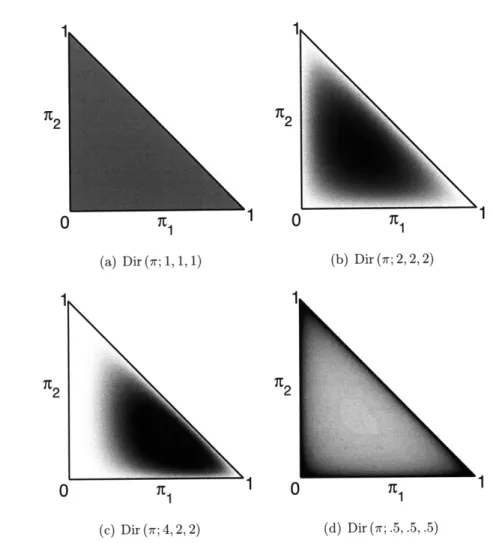
(N + Ek k) k (ak)

The hyperparameters ak can be thought of as a prior/pseudo count of how many times one saw the value K in Ek ak trials. Figure 2.5 shows several Dirichlet distributions

using different hyperparameters.

* 2.4.2 Normal Distribution

Perhaps the most commonly used distrib ution for continuous valued random vectors x whose values are in Rd is the Gaussian or normal distribution. Given parameters 0 = {p, A} it takes the form:

p (xIO) = f (x; p, A) (2.34)

S(2)d/2 _exp_{(x _- _p)TA-l(x

- p) _(2.35)

(27)d/21/2 2

where p E Rd is the mean and A E Rdxd is a d x d positive definite matrix representing

the covariance among the elements in x.

Given N independent samples of x in D, the ML estimate of the Gaussian's param-eters are the sample mean and covariance:

N N

(39)

Sec. 2.4. Parameterization, Learning, Inference and Evidence JU

1

0 I

1

0

(a) Dir (ir; 1, 1, 1) (b) Dir (7r; 2, 2, 2)

0 xL

₁

(c) Dir (7r; 4, 2, 2) (d) Dir (7; .5, .5, .5)

Figure 2.5. Example Dirichlet Distributions: Distributions for K = 3 are displayed on the simplex

(rl, 72,1 - 71 - 72). Dark represents high probability. (a) Uniform prior, (b) Prior biased toward equal

7rks (c) Prior biased toward K = 1, (c) By setting ak < 0 one obtains a prior that favors a sparse 7r.

Normal-Inverse-Wishart Distribution

The conjugate prior for the normal distribution is the normal-inverse- Wishart distribu-tion. It factorizes as a normal prior on the mean given the covariance and an inverse-Wishart prior on the covariance given hyperparameters T = {w, K, E, v}:

Po

(oIT)

= Po (pIA,

T)

po (AT)

= .AF (1; w, A/,) ZW (A; E, v)

(2.37)

(2.38)

(40)

Here the conditional prior on p is a Gaussian with an expected value of w E Rd and covariance scaled by r, E R1. The hyperparameter r can be thought of a count of prior

"pseudo-observations." The higher r is the tighter the prior on p becomes around its mean w. The d-dimensional inverse-Wishart distribution with positive definite param-eter E E Rdx d and v E R1 degrees of freedom has the form:

|pv/2 A j- 2lexp {-ltr (EA-') }

1W (A; Z, v)= vd (2.39)

2 2 _{d(d-1)/4 fj=1} ₍ _-2

The expected value of this distribution is simply E/(v - d - 1). It can be shown that, given N independent Gaussian observations the posterior distribution has the form:

p (o|D, T) = N (p; w, A/ ) ZW (A; 2, 0) (2.40)

where the updated hyperparameters are

= + N (2.41) =v + N (2.42) N n 1

Nw-

+ N Dn (2.43) +N +N n=l N 2 +

.

DD T + KW T D . (2.44) n=l

Figure 2.6 shows an example normal-inverse-Wishart prior and an associated posterior given samples drawn from a normal distribution.

Integrating out parameters, the evidence takes the form:

Id F ((v + N + I - i)/2) d/2 v/2

p (D T) - 1= 1 ( N 1(2.45)

i=I F ((v + 1 - i)/2) + N Nd12 (v+N)/2

This is an evaluation of a multivariate-T distribution. We will show this is a special case of the more general matrix-T distribution in the next section.

N 2.4.3 Matrix-Normal Distribution

Next consider the case when one needs to model a conditional distribution p (yIx) where y E Rd and x E Rm . The normal distribution can be generalized to model a linear Gaussian relationship such that

(41)

Sec. 2.4. Parameterization, Learning, Inference and Evidence 41i 4 4 4 2 2 2

X

0 X X Xo

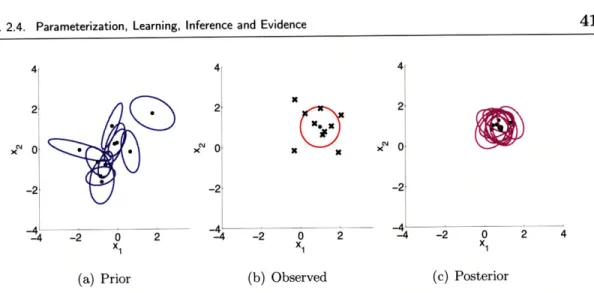
-2 -2 -2 -4-4 -4 -4 -2 0 2 -4 -2 0 2 -4 -2 0 2 4 X₁ X1 X1

(a) Prior (b) Observed (c) Posterior

Figure 2.6. Examples of the Normal-Inverse-Wishart distribution: (a) Shows 10 2-d normal distri-butions with their parameters samples from a normal-inverse-wishart prior KN (p; 0, 2A) ZW (A; 12, 5). Black dots represent the mean and the covariance is plotted as an ellipse. (b) Samples from a normal distribution with mean [1 1]T and covariance 12. (c) Gaussians with their parameters sampled from the posterior on parameters given the samples in (b).

where A E Rdxm and the random variable e E Rd is drawn from a zero mean normal

distribution with covariance A. The conditional distribution is thus

p (y x,

E)

= N (y; Ax, A) . (2.47)

Under this model the ML parameter estimates given N observations of y and x, D)Y

and DX are

(-1

^E= ( DnT mD T (2.48) () (

-)

T (2.49) n=1 Matrix-Normal-Inverse-Wishart Distribution

The conjugate prior for this model is a generalization of the normal-inverse-Wishart distribution. Given T = {I, K, E, K, v} a matrix-normal-inverse- Wishart distribution has the form

Dynamic dependence analysis : modeling and inference of changing dependence among multiple time-series

Dynamic Dependence Analysis

:

Modeling and Inference of

Changing Dependence Among Multiple Time-Series

©

AUG 0 7

2009

LIBRARIES

ARCHIVES

Dynamic Dependence Analysis

:

Modeling and Inference of

Changing Dependence Among Multiple Time-Series

Acknowledgments

Contents

List of Figures

Quantization

#

List of Tables

List of Algorithms

Chapter 1

Introduction

* 1.1 Motivation

* 1.2 Objective

* 1.3 Our Approach

* 1.5 Organization of this Dissertation

Chapter 2

Background

2.1 Statistical Dependence

2.2 Graphical Models

j)

j)

j

j)

j.

j

X2

X1

X2

X1

X

X1

X2

X3X3

X3

X3

X4

X4

Z = Z I-bf(xf)

(2.8)

4

* 2.2.3 Undirected Graphical Models

0,

(X

p (X1:T) = p

(xt

X1:t-1)

(2.14)

fp

E

E

E

E

eilpa(i)

E.

E,

IE,

it part of O.

E

E.

0*

p(D) =

p(DO) po

(0

T) dO

(2.21)

p() =

(D ) po (

IT)

_(2.25)