HAL Id: hal-02564838
https://hal.inrae.fr/hal-02564838
Submitted on 6 May 2020
HAL is a multi-disciplinary open access
archive for the deposit and dissemination of
sci-entific research documents, whether they are
pub-lished or not. The documents may come from
teaching and research institutions in France or
abroad, or from public or private research centers.
L’archive ouverte pluridisciplinaire HAL, est
destinée au dépôt et à la diffusion de documents
scientifiques de niveau recherche, publiés ou non,
émanant des établissements d’enseignement et de
recherche français ou étrangers, des laboratoires
publics ou privés.
O. Clifton, F. Paulot, A. Fiore, L. Horowitz, G. Correa, C. Baublitz, S. Fares,
I. Goded, A. Goldstein, C. Gruening, et al.
To cite this version:
O. Clifton, F. Paulot, A. Fiore, L. Horowitz, G. Correa, et al.. Influence of dynamic ozone dry
deposition on ozone pollution. Journal of Geophysical Research: Atmospheres, American Geophysical
Union, 2020, 125 (8), �10.1029/2020JD032398�. �hal-02564838�
O. E. Clifton1,2,3 , F. Paulot4,5 , A. M. Fiore1,2 , L. W. Horowitz4 , G. Correa2,
C. B. Baublitz1,2 , S. Fares6,7 , I. Goded8, A. H. Goldstein9 , C. Gruening8, A. J. Hogg10,
B. Loubet11 , I. Mammarella12 , J. W. Munger13 , L. Neil14, P. Stella15, J. Uddling16,
T. Vesala12,17 , and E. Weng18,19
1Department of Earth and Environmental Sciences, Columbia University, New York, NY, USA,2Lamont-Doherty Earth
Observatory of Columbia University, Palisades, NY, USA,3Advanced Study Program, National Center for Atmospheric
Research, Boulder, CO, USA,4Geophysical Fluid Dynamics Laboratory, National Oceanic and Atmospheric
Administration, Princeton, NJ, USA,5Program in Atmospheric and Oceanic Sciences, Princeton University, Princeton,
NJ, USA,6Council of Agricultural Research and Economics, Research Centre of Forestry and Wood, Rome, Italy,
7Institute of Bioeconomy, National Research Council, Rome, Italy,8Joint Research Centre, European Commission,
Ispra, Italy,9Department of Environmental Science, Policy, and Management, University of California, Berkeley, Berkeley, CA, USA,10Program in Technical Communication, College of Engineering, University of Michigan, Ann
Arbor, MI, USA,11National Institute for Agronomic Research UMR INRA/AgroParisTech ECOSYS, Université
Paris-Saclay, Thiverval-Grignon, France,12Institute for Atmospheric and Earth System Research/Physics, University of
Helsinki, Helsinki, Finland,13School of Engineering and Applied Science and Department of Earth and Planetary
Sciences, Harvard University, Cambridge, MA, USA,14Hemmera, Ausenco, Oakville, Ontario, Canada,15UMR SAD-APT, AgroParisTech, INRA, Université Paris-Saclay, Paris, France,16Department of Biological and Environmental
Sciences, University of Gothenburg, Gothenburg, Sweden,17Institute for Atmospheric and Earth System
Research/Forest Sciences, University of Helsinki, Helsinki, Finland,18Center for Climate Systems Research, Columbia
University, New York, NY, USA,19NASA Goddard Institute for Space Studies, New York, NY, USA
Abstract
Identifying the contributions of chemistry and transport to observed ozone pollution using regional-to-global models relies on accurate representation of ozone dry deposition. We use a recently developed configuration of the NOAA GFDL chemistry-climate model—in which the atmosphere and land are coupled through dry deposition—to investigate the influence of ozone dry deposition on ozone pollution over northern midlatitudes. In our model, deposition pathways are tied to dynamic terrestrial processes, such as photosynthesis and water cycling through the canopy and soil. Small increases in winter deposition due to more process-based representation of snow and deposition to surfaces reduce hemispheric-scale ozone throughout the lower troposphere by 5–12 ppb, improving agreement with observations relative to a simulation with the standard configuration for ozone dry deposition. Declining snow cover by the end of the 21st-century tempers the previously identified influence of rising methane on winter ozone. Dynamic dry deposition changes summer surface ozone by −4 to +7 ppb. While previous studies emphasize the importance of uptake by plant stomata, new diagnostic tracking of depositional pathways reveals a widespread impact of nonstomatal deposition on ozone pollution. Daily variability in both stomatal and nonstomatal deposition contribute to daily variability in ozone pollution. Twenty-first century changes in summer deposition result from a balance among changes in individual pathways, reflecting differing responses to both high carbon dioxide (through plant physiology versus biomass accumulation) and water availability. Our findings highlight a need for constraints on the processes driving ozone dry deposition to test representation in regional-to-global models.1. Introduction
In the troposphere, ozone is an air pollutant, a potent greenhouse gas, and an important source of the hydroxyl radical, the main tropospheric oxidant. Regional-to-global atmospheric chemistry models are key tools for quantifying the impacts of ozone pollution on human and vegetation health and pinpointing the drivers of observed trends and variability in tropospheric constituents. Representing ozone sources and sinks accurately in these models is fundamental to their utility. Ozone dry deposition is an important (20% of the annual global tropospheric loss), but uncertain and frequently overlooked, tropospheric ozone Key Points:
• Remote and local ozone depositional sinks shape regional winter ozone pollution • Dynamic ozone dry deposition
changes summer surface ozone over northern midlatitude regions by
−4 to+7 ppb
• Variability and 21st-century changes in both stomatal and nonstomatal deposition influence summer surface ozone distributions
Supporting Information: • Supporting Information S1 • Figure S1 • Figure S2 • Figure S3 • Figure S4 Correspondence to: O. E. Clifton, oclifton@ucar.edu Citation:
Clifton, O. E., Paulot, F., Fiore, A. M., Horowitz, L. W., Correa, G., Baublitz, C. B., et al. (2020). Influence of dynamic ozone dry deposition on ozone pollution. Journal of
Geophysical Research: Atmospheres,
125, e2020JD032398. https://doi.org/ 10.1029/2020JD032398
Received 6 JAN 2020 Accepted 20 MAR 2020
Accepted article online 4 APR 2020
Author Contributions
Conceptualization: O. E. Clifton,
A. M. Fiore
Data curation: O. E. Clifton,
F. Paulot, A. M. Fiore, L. W. Horowitz, G. Correa, C. B. Baublitz, S. Fares, I. Goded, A. H. Goldstein, C. Gruening, A. J. Hogg, B. Loubet, I. Mammarella, J. W. Munger, L. Neil, P. Stella, J. Uddling, T. Vesala, E. Weng
Funding Acquisition: O. E. Clifton,
A. M. Fiore
Methodology: O. E. Clifton, F. Paulot,
L. W. Horowitz, G. Correa, E. Weng
©2020. American Geophysical Union. All Rights Reserved.
sink (Hardacre et al., 2015; Wild, 2007). Here we investigate the role of ozone dry deposition on ozone pol-lution at northern midlatitudes with a global chemistry-climate model that leverages the carbon and water cycling in its underlying dynamic vegetation land model for representing dry deposition.
Dry deposition of ozone occurs through surface-mediated reactions after diffusion through plant stomata, or on leaf cuticles, other plant material, soil, water, and snow. Ozone deposition velocity (a measure of the efficiency of the removal independent from ambient ozone concentration) is typically highest during summer, reflecting uptake by vegetation. Winter ozone dry deposition is usually not a research focus due to relatively low ozone deposition velocity. However, the long winter ozone lifetime implies efficient transport through large-scale circulation patterns, such that ozone at any particular location depends on both local and remote sources and sinks and thus may be sensitive to changes in ozone dry deposition locally and upwind. Although previous studies examine the sensitivity of winter ozone abundances to ozone deposition velocity over the Uintah Basin in the western United States (Matichuk et al., 2017) and boreal and Arctic regions (Helmig et al., 2007), it is unknown how ozone dry deposition impacts large-scale winter ozone pollution over northern midlatitudes. While ozone pollution is typically regarded as a summer problem (at least over polluted and populated regions), projected changes in anthropogenic precursor emissions drive large 21st-century increases in winter ozone pollution (Clifton et al., 2014; Gao et al., 2013; Rieder et al., 2018), implying a need to advance understanding of winter sources and sinks.
Much of the attention around ozone dry deposition is on its influence on summer ozone pollution. Previous work examines changes in ozone dry deposition with environmental conditions, ambient carbon dioxide, and land use/land cover as well as the impact of dry deposition on summer surface ozone (Andersson & Engardt, 2010; Anav et al., 2018; Fu & Tai, 2015; Ganzeveld et al., 2010; Geddes et al., 2016; Heald & Geddes, 2016; Hollaway et al., 2016; Huang et al., 2016; Lin et al., 2019; Solberg et al., 2008; Trail et al., 2015; Wong et al., 2019; Wu et al., 2012). The aforementioned analyses linking surface ozone with ozone dry deposition all rely on models. These models typically assume that stomatal uptake dominates ozone dry deposition and that nonstomatal deposition is roughly constant or simply varies with leaf area index (LAI). However, laboratory and field evidence suggests that these assumptions may limit our ability to model ozone dry deposition accurately (Altimir et al., 2006; Cieslik, 2009; Clifton et al., 2017, 2019; Fares et al., 2010, 2012, 2014; Fowler et al., 2009; Fuentes et al., 1992; Fumagalli et al., 2016; Massman, 2004; Potier et al., 2015; Potier et al., 2017; Rannik et al., 2012; Stella et al., 2011, Sun et al., 2016). Current understanding of nonstomatal deposition pathways is that leaf cuticular uptake increases with leaf wetness, soil uptake decreases with soil moisture, and snow on vegetation and the ground decreases uptake (Clifton et al., 2020). Systematic omissions in process representation that lead to variations in ozone deposition velocity with meteorology or biophysics may impede accurate model simulations of changes in ozone pollution attributable to changes in dry deposition.
Here we probe the influence of ozone dry deposition on winter and summer ozone pollution over north-ern midlatitudes under a 21st-century scenario for climate and anthropogenic emissions of pollutants and their precursors using a new configuration of the global National Oceanic and Atmospheric Administra-tion (NOAA) Geophysical Fluid Dynamics Laboratory (GFDL) chemistry-climate model. In particular, we use the biophysics of the land component to simulate ozone dry deposition by plant stomata, stems, and wet, dry, and snow-covered soil and leaf cuticles. We evaluate this model with ozone eddy covariance flux observations from long-term and short-term data sets and estimates of the stomatal fraction of ozone dry deposition derived from observations. We compare simulations with this new dynamic ozone dry deposition scheme to simulations using a prescribed climatology of ozone deposition velocity, the default configuration in the GFDL model. While nonstomatal deposition pathways represent observed dependencies on meteo-rological and biophysical variables in our model to the extent possible, these pathways remain uncertain due to a paucity of observational constraints, and their representation in models is highly parameterized (Clifton et al., 2020). Our goal is to investigate how dynamic ozone dry deposition, based on current understanding, influences ozone pollution.
2. Methods
We conduct time-slice simulations for the 2010s and 2090s with the NOAA GFDL atmospheric model ver-sion 3 (AM3) coupled to the NOAA GFDL land model verver-sion 3 (LM3) through not only carbon, water, and energy exchanges but also dry deposition of several atmospheric constituents (AM3DD) (Paulot et al., 2018).
Validation: O. E. Clifton Writing - Original Draft:
O. E. Clifton
Formal Analysis: O. E. Clifton Investigation: S. Fares, I. Goded,
A. H. Goldstein, C. Gruening, A. J. Hogg, B. Loubet, I. Mammarella, J. W. Munger, L. Neil, P. Stella, T. Vesala
Resources: L. W. Horowitz Supervision: A. M. Fiore Visualization: O. E. Clifton Writing - review & editing:
O. E. Clifton, F. Paulot, A. M. Fiore, L. W. Horowitz, C. B. Baublitz, B. Loubet, I. Mammarella, P. Stella
Each simulation contains 10 years. Below we describe the model configuration and the dynamic dry depo-sition scheme for ozone, which we modify from the general dynamic dry depodepo-sition scheme described by Paulot et al. (2018).
AM3 is a chemistry-climate model with online fully coupled stratospheric and tropospheric chemistry (Donner et al., 2011; Naik et al., 2013). We use AM3 with C48 (cubed sphere) configuration (∼2◦by 2◦) and 48 vertical levels. We update the treatment of wet deposition of aerosols and gases in AM3 following Paulot et al. (2016); in particular, snow formed by the Bergeron process does not scavenge water-soluble aerosols. We use Representative Concentration Pathway 8.5 (RCP8.5) (Lamarque et al., 2011; Riahi et al., 2011; van Vuuren et al., 2011), the high-warming scenario designed for the Coupled Model Intercomparison Project 5 (CMIP5), to represent 21st-century climate and anthropogenic emissions. Aerosol and ozone pre-cursor emissions and global concentrations of greenhouse gases are set to 2010 and 2090 levels for our 2010s and 2090s time-slice simulations, respectively. Isoprene emissions are calculated online with a version of Model of Emissions of Gases and Aerosols from Nature (MEGAN) in AM3 (Emmons et al., 2010; Guenther et al., 2006; Rasmussen et al., 2012). Simulations are forced with decadal mean (2011–2020 or 2091–2100) sea ice and sea surface temperatures from transient RCP8.5 simulations (average over three ensemble mem-bers) from the NOAA GFDL coupled model version 3 (CM3). We use initial conditions for 2010 and 2090 from one ensemble member of the transient 21st-century RCP8.5 CM3 simulations described in Clifton et al. (2014) that were spun up from a preindustrial control simulation (John et al., 2012).
LM3 is a global land model with terrestrial carbon, energy and water cycling, dynamic vegetation, and land use transitions (Milly et al., 2014; Shevliakova et al., 2009). A subgrid tiling framework in LM3 allows individual tiles to represent distinct land uses, including primary vegetation, cropland, pasture, secondary vegetation, and bodies of water and glaciers. We prescribe land use distributions with either 2010 or 2090 RCP8.5 (Hurtt et al., 2011). Primary vegetation has never been disturbed by humans directly, whereas sec-ondary vegetation has been harvested and subsequently abandoned at least once. Each grid cell contains up to 12 stages of secondary vegetation, allowing for differing recovery times. Modifications to crop harvesting and pasture grazing follow Paulot et al. (2018). Each vegetated subgrid tile has one land cover type. Land cover types include temperate deciduous forests, tropical forests, cold coniferous forests, C3grass, and C4
grass. The distribution of vegetation evolves with climate, but the distribution of bodies of water and glaciers is time invariant. There are five pools of vegetation biomass (leaves, fine roots, sapwood, heartwood, and labile stores), and allocation rules and daily net primary production update the pools each day (Shevliakova et al., 2009). Phenology (i.e., leaf on/off) and thus LAI is updated monthly from the leaf biomass pool accord-ing to monthly mean air temperature and soil water available to the plant (Shevliakova et al., 2009) except for temperate deciduous vegetation, for which LAI has strong seasonality. We update the temperate deciduous vegetation daily according to critical temperature and growing degree day following Weng et al. (2015).
2.1. Ozone Dry Deposition in AM3DD
The new ozone dry deposition parameterization in LM3 uses a big-leaf resistance framework. Pathways for ozone dry deposition include leaf cuticles, stomata, stems, and the ground. Ozone deposition velocity (vd)
[cm s−1] follows: vd= ⎡ ⎢ ⎢ ⎢ ⎢ ⎣ Ra+ 1 1 Rb,v+ 1 1 Rcut+Rstom+Rmeso1 + 1 Rb,v+Rstem + 1 Rac,g+Rb,g+Rg ⎤ ⎥ ⎥ ⎥ ⎥ ⎦ −1 ∗100 (1)
In the following paragraphs, we define each resistance term in equation (1). The scheme follows Paulot et al. (2018) except where otherwise noted.
The resistance to turbulent transport between the atmosphere and canopy (Ra) [s m−1] follows Fick's Law
and Monin-Obukhov Similarity Theory. The quasi-laminar boundary layer resistance for vegetation (Rb,v)
[s m−1] follows Choudhury and Monteith (1988) and Bonan (1996):
Rb,v=a b √ dleaf uh 1 [1 − e−a∕2] (Sc Pr )2∕3 (2)
The parameter dleafis the leaf dimension [m]; uhis wind speed at the top of the canopy [m s−1] (h is canopy
height [m]); a is an empirical constant (value of 3); b [m s−0.5] is an empirical constant (value of 0.02); Sc is
the Schmidt number [unitless]; Pr is the Prandtl number [unitless]. Rb,vis scaled by fraction of vegetation
that is stems versus leaves when used in equation (1).
Paulot et al. (2018) apply both equation (2) and the Jensen and Hummelshøj (1995, 1997) Rb,v parameter-ization, with the intention of including a resistance to in-canopy turbulence. However, equation (2) is a quasi-laminar boundary layer resistance, not a resistance to in-canopy turbulence. We use equation (2) for Rb,vbecause it is used for energy and carbon exchanges in LM3. A resistance to in-canopy turbulence for
leaf deposition is unnecessary in our big-leaf model because Raaccounts for turbulent transport between
the atmosphere and canopy and all vegetation is assumed to be at the canopy height.
We distinguish cuticular deposition among dry, wet, and snow-covered leaves. Fractional leaf wetness is calculated from canopy-intercepted water, specifically the ratio of canopy-intercepted water to the maximum storage capacity to the two-thirds power (Bonan, 1996). Fractional snow cover on vegetation is calculated in the same way but with canopy-intercepted snow. We employ an adjustment function s [unitless] to reduce wet and dry cuticular deposition when leaf temperatures are cold (<5◦C).
s(Tleaf) =max[e−c(Tleaf−5), 1] (3)
The variable Tleaf is leaf temperature [◦C]; c is a constant [◦C−1]. Such an adjustment function assumes
that the chemistry on surfaces is slower when the surfaces are cold. We use c = 0.9◦C−1for wet and c =
0.1◦C−1for dry cuticular deposition, employing different values because the initial resistances for wet and
dry cuticular deposition differ by an order of magnitude (see below). Our temperature adjustment function, an adaptation of Zhang et al. (2003), allows for cuticular deposition at cold temperatures to be reduced, but not turned off. We do not turn off cuticular deposition on cold surfaces following observational evidence that uptake occurs on material protruding from snow (Clifton et al., 2020).
Paulot et al. (2018) use the Zhang et al. (2003) temperature adjustment function. Without our change to the Zhang et al. (2003) temperature adjustment function, winter cuticular uptake to coniferous forests (only in boreal regions in LM3) becomes higher than that supported by field observations. For example, sim-ulated winter mean vdover boreal regions (55–65◦N) with LAI≥ 2 m2m−2is 0.1 cm−1with this temperature
adjustment function, only slightly less than observations from Hyytiälä, a boreal coniferous forest, which suggest a winter mean vdof 0.12 cms−1. Previous studies do not identify the need for a stronger temperature
adjustment function, likely because they assume vegetation in winter boreal regions to be completely snow covered, whereas here we consider dynamic canopy cycling of snow. Canopy snow cycling in LM3 allows conifers to be occasionally snow-free, leading us to implement a stronger temperature adjustment function to reduce otherwise unrealistically high simulated uptake to snow-free conifer cuticles.
The resistance to cuticular deposition to dry leaves (Rcut,dry) [s m−1] follows:
Rcut,dry=
Ri,cut,dry
LAIeRHs(Tleaf) (4)
The parameter Ri,cut,dryis the initial resistance to dry cuticular deposition [s m−1]; RH is fractional in-canopy
relative humidity [unitless]. The RH dependence is an update to Paulot et al. (2018) and follows field and lab-oratory evidence suggesting that ozone dry deposition to cuticles occurs through aqueous surface-mediated chemistry (Fuentes et al., 1992; Potier et al., 2015, 2017; Sun et al., 2016; Zhang et al., 2002). In particular, the RH dependence in the model for Rcut,dryrepresents the thin water films that form on leaves at high ambient humidity (Burkhardt & Hunsche, 2013).
Higher ozone deposition to leaves wet by rain and dew (Clifton et al., 2020) is also accounted for in our model. The resistance to cuticular deposition to leaves wet by rain and dew (Rcut,wet) [s m−1] follows:
Rcut,wet=
Ri,cut,wet
LAI s(Tleaf) (5)
The parameter Ri,cut,wetis the initial resistance to wet cuticular deposition [s m−1]. For pastures, crops, and
trees, Ri,cut,dryis 6,000 s m−1and Ri,cut,wetis 400 s m−1. Initial resistances follow Zhang et al. (2003), except that
initial resistances for coniferous trees are the same for other trees, not much lower as suggested by Zhang et al. (2003). Paulot et al. (2018) originally implemented the initial resistances suggested by Zhang et al. (2003) for conifers, but increasing the initial resistances for conifers to agree with the values for other trees reduces dry deposition to coniferous forests (only in boreal regions in LM3) where LM3 overestimates LAI. We note that the Zhang et al. (2003) initial resistances were derived from observations from one growing season or less in eastern United States locations, and thus their application more generally for global land use types is highly uncertain.
The resistance to cuticular deposition to snow-covered leaves (Rcut,snow) [s m−1] follows:
Rcut,snow= Ri,snow
LAI (6)
The parameter Ri,snow, the initial resistance to snow, is 7,000 s m−1. Often the number of surfaces covered by
snow is not considered in models of ozone dry deposition (i.e., Rcut,snow=Ri,snow). Our model (equation (6)) assumes deposition increases with LAI [m2m−2], implying higher deposition to a larger surface area covered
with snow. This relationship is supported by observations of relatively high vdover snow-covered forests (Neirynck & Verstraeten, 2018; Padro, 1993; Padro et al., 1992; Wu et al., 2016).
Our value for Ri,snowis more than triple the 2,000 s m−1used by Paulot et al. (2018) and given by Zhang et al.
(2003). Increasing Ri,snowleads to uptake by snow on the ground and leaf cuticles of 0.015 cm s−1on average
over 40–65◦N for present-day winter. Most field and laboratory observations support vdover snow between 0 and 0.1 cm s−1(Aldaz, 1969; Clifton et al., 2020; Colbeck & Harrison, 1985; Galbally & Allison, 1972;
Galbally & Roy, 1980; Gong et al., 1997; Helmig et al., 2009; Hopper et al., 1998; Stocker et al., 1995; Wesely et al., 1981). In our model, vdover places with snow includes not only deposition to snow-covered ground and leaf cuticles but also deposition to stems as well as any snow-free leaf cuticles and ground. Winter mean vdacross 40–65◦N only including grid cells with 10% or greater snow cover for leaves or ground is 0.1 cm s−1.
The calculation of stomatal resistance (Rstom) [s m−1] for water vapor (Leuning, 1995) is coupled with the
calculation of net photosynthesis (Anet) [mol CO2m−2s−1] (Collatz et al., 1991, 1992; Farquhar et al., 1980):
Rstom= ps RTleaf 1 m ( 1 + ds d0 ) ci−𝛤 Anet 1 LAI (7)
The variable psis surface pressure [Pa]; R is the universal gas constant [J mol air−1K−1]; m is an empirical
constant [unitless]; dsis the humidity deficit [kg H2O kg air−1]; d
0is another empirical constant [kg H2O kg
air−1]; c
iis carbon dioxide concentration internal to the leaf [mol CO2mol air−1];𝛤 is carbon dioxide
com-pensation point [mol CO2mol air−1]; R
stomshown in the above equation is also scaled by the inverse of the
fractional water stress if the fractional water stress<1 (Milly et al., 2014). The water stress is the ratio of water supply to roots to water demand from atmosphere.
We account for the different diffusivities of ozone and water vapor by scaling Rstomgiven in equation (7) for
water vapor by the ratio of the diffusivities of the two gases. The resistance to ozone reacting with internal fluids and tissues in our model (i.e., often called a mesophyll resistance, or Rmeso[s m−1]) is small (0.01 s m−1)
because laboratory evidence suggests that ozone reacts immediately upon entering stomata (Laisk et al., 1989; Wang et al., 1995).
Stomatal deposition is reduced on the part of the leaf that is wet by dew or rain; this happens through a 30% decrease in Anetand stomatal conductance on the wet part of the leaf. This is a correction to Paulot et al.
(2018) and Lin et al. (2019) who reduce stomatal deposition by the fraction of the leaf that is wet in addition to the 30% decrease in Anetand stomatal conductance that we retain here.
The stem resistance (Rstem) to ozone dry deposition is:
Rstem=
Ri,stem
SAI (8)
The parameter Ri,stem is 3,000 s m−1; SAI [m2 m−2] is stem area index. While Paulot et al. (2018) use
cold surfaces, our change to Ri,stemand removal of the temperature adjustment function allow for higher
deposition to stems and distinguishing between winter deposition to vegetated versus nonvegetated regions (Clifton et al., 2020). The latter also allows for slightly higher winter deposition to bare deciduous trees relative to areas without woody biomass, as supported by observations (Clifton et al., 2020; Padro et al., 1992). A resistance to in-canopy turbulence influences dry deposition to the ground when vegetation is present (LAI + SAI>0.25 m2m−2) and follows Paulot et al. (2018). The model was developed from a very short-term
regression analysis over a corn field (Van Pul & Jacobs, 1994), but has been used widely in dry deposition schemes (Emberson et al., 2000; Erisman et al., 1994; Pleim & Ran, 2011; Zhang et al., 2002). We use this Rac,gparameterization because there are not many alternatives for large-scale big-leaf modeling.
Rac,g= 14(LAI + SAI)h u∗
(9)
The variable u*is friction velocity [m s−1]. The number 14 is a constant fit via regression and has units of
m−1. Instead of setting LAI to unity when trees are leafless as Erisman et al. (1994) do, we replace LAI with
LAI + SAI for all conditions. If vegetation is not present, Rac,gis negligible (0.01 s m−1).
The quasi-laminar boundary layer resistance for all ground surfaces (Rb,g) [s m−1] except lakes follows
Wesely and Hicks (1977) implemented by Paulot et al. (2018): Rb,g= 2 ku∗ (Sc Pr )2∕3 (10)
The parameter k is the von Kármán constant [unitless]. If vegetation is present then u*near the ground (u*,g) [m s−1] is used in equation (10). u∗,g=u∗e0.6(LAI+SAI) (z0,g h −1 ) (11) The parameter z0,g is the roughness length of the ground for scalars [m] as calculated in Bonan (1996).
Equation (11) follows Loubet et al. (2006) but also includes SAI, allowing bare trees to contribute to drag. For very low vegetation (h< 0.1 m), we assume u∗,g=u*.
The quasi-laminar boundary-layer resistance for lakes (Rb,g,lake) [s m−1] follows Hicks and Liss (1976):
Rb,g,lake= ln ( z0,g DO3ku∗ ) ku∗ (12) The parameter DO
3is the diffusivity of ozone in air [m 2s−1].
We distinguish dry deposition to the ground among snow-covered, wet, and dry soil, deserts, lakes, and glaciers. While a synthesis across observations suggests that ground deposition depends on soil moisture (Massman, 2004), the exact relationship is unknown. We thus prescribe a simple step function such that ground uptake decreases when soil is wet as suggested by Massman (2004). We define wet soil as fractional surface soil moisture in a tile>0.9. Some work points to an exponential or logarithmic dependence of ground deposition with moisture (Fumagalli et al., 2016; Stella et al., 2011, 2019), but we maintain a simpler change in ground deposition due to poor understanding of what happens at the large scale.
The treatment of ground deposition to cold surfaces from Paulot et al. (2018) considers the ground to be covered with snow if there is any snow in a tile and employs the Zhang et al. (2003) temperature adjustment function to reduce ground deposition at cold temperatures. Instead, we update the model to use fractional snow cover on the ground, calculated as a function of snow depth and prescribed critical depth as done for surface albedo. We change the temperature adjustment function to the one used for cuticles (equation (3)) and use c = 0.025◦C−1and soil temperature (T
soil) [◦C]. We maintain the Paulot et al. (2018) treatment of
frozen lakes: Lakes are frozen if there is any solid water. The resistance to ground deposition (Rg) [s m−1] follows:
The parameter Ri,g[s m−1] is the initial resistance to ground deposition. Ri,gfor snow and ice is Ri,snow
(7,000 s m−1). R
i,gfor wet surfaces (e.g., lakes, wet soil) is 500 s m−1and dry vegetated surfaces is 200 s m−1
(Zhang et al., 2003). Ri,gfor deserts (defined by<0.05 kg m−2biomass) is 500 s m−1. Ozone dry deposition to
the ground is largely considered to occur through reaction with soil organic material, but short-term obser-vations suggest nonnegligible uptake over the Sahara Desert (Güsten et al., 1996). However, relationships between soil organic content and ozone dry deposition to the ground are poorly constrained, leading to major uncertainties in representing dry deposition in different dry environments. Paulot et al. (2018) define Ri,gfor deserts to be 500 s m−1, but their desert definition is broader (<0.25 kg m−2biomass). Our changes
to ground deposition to deserts in part reflect the need for nonnegligible deposition in regions such as the western United States where otherwise vdin LM3 is too low due to inaccurate representation of vegetation
there.
In order to probe the contribution of different deposition pathways to vd, we examine effective conductances. Generally, a conductance is the inverse of a resistance. The effective conductance is the amount of deposition (in velocity units) occurring through a given deposition pathway. The sum of all of the effective conductances is vd.
Dry deposition to the ocean in AM3DD follows monthly average fields from GEOS-Chem, a widely used chemical transport model. Aside from the meteorological dependencies of the resistances to turbulent trans-port and the quasi-laminar boundary layer between the ocean and atmosphere, vdin GEOS-Chem over oceans does not change with meteorology, sea surface temperatures, or surface-mediated chemistry in con-trast to observational evidence (Ganzeveld et al., 2009; Helmig et al., 2012; Luhar et al., 2017; Martino et al., 2012; Sarwar et al., 2016).
2.2. Sensitivity Simulation With Default Configuration for Ozone Dry Deposition
In addition to AM3DD simulations with dynamic ozone dry deposition, we examine AM3DD simulations where we prescribe a monthly mean climatology of vdscaled to a diel cycle (hereafter, AM3DD-staticO3DD), which is the default configuration for the GFDL model (Naik et al., 2013; Paulot et al., 2016). The clima-tology is single-year monthly average fields from a widely used chemical transport model, GEOS-Chem. We impose the multiyear monthly mean diel cycle from AM3DD 2010s. Differences between AM3DD and AM3DD-staticO3DD at the 2010s reflect differences in interannual, daily, and spatial variability in vdrather
than the diel cycle. AM3DD-staticO3DD for the 2090s uses the same setup for vdas AM3DD-staticO3DD for the 2010s, which allows us to consider how neglecting 21st-century changes in vdimpacts surface ozone projections.
Briefly, the vdclimatology was generated with GEOS-Chem, which uses a modified Wesely (1989) dry
depo-sition scheme (Wang et al., 1998). Rafollows Fick's Law and Monin-Obukhov Similarity Theory (specifically, Businger et al., 1971). Rbis not specific to any surface and follows Wesely and Hicks (1977). Rgand Rac,gare time-invariant, but change with land cover type. Ozone dry deposition to cuticles varies with LAI and land cover type. Land cover type follows the Olson et al. (2001) land map. Stomatal ozone dry deposition varies with LAI, light, temperature, and land cover type (Wang et al., 1998). This scheme has a deposition path-way to the ground as well as to the lower canopy. High albedo (>0.4) is used as a proxy for snow-covered surfaces to which ozone dry deposition is inhibited. The temperature adjustment function for cold surfaces in GEOS-Chem follows Wesely (1989).
3. Model Evaluation of Dynamic Ozone Dry Deposition
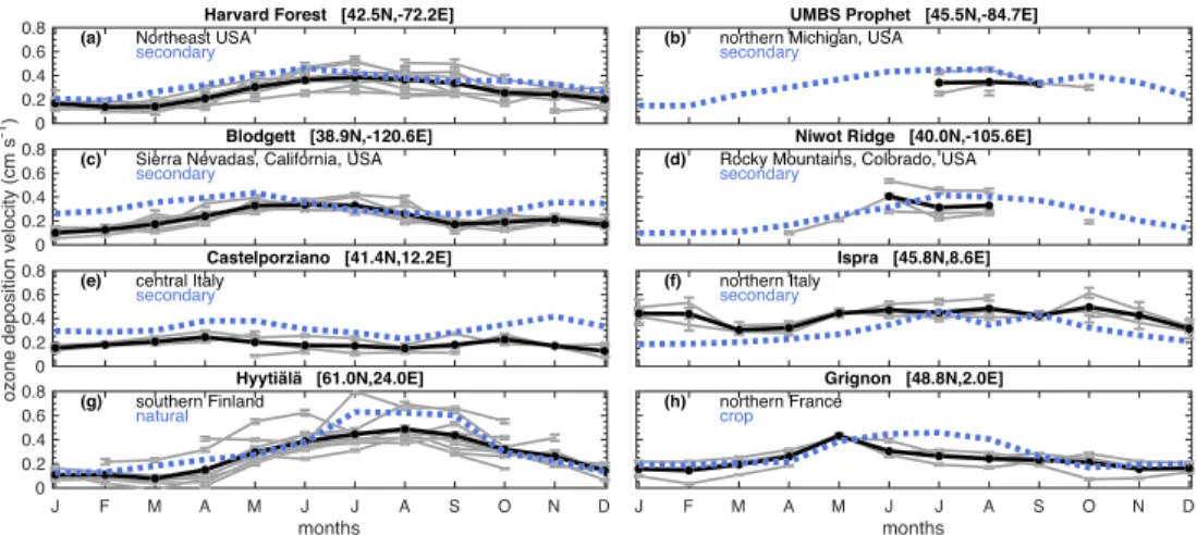
We compare monthly mean vdfrom ozone eddy covariance fluxes at observational sites (Table 1) with vd simulated by AM3DD (Figures 1 and 2). We archive simulated vdfor each land use type within a grid cell (recall subtiling framework described above), which allows for a more direct comparison with observations (e.g., Paulot et al., 2018; Silva & Heald, 2018). The model land use type that best matches the observational site is selected for the evaluations in Figures 1 and 2. We focus our model evaluation on the eight sites with multiple years of data and at least a couple of months of data collected in a given year (Figure 1). At these sites, monthly daily mean vdshows strong interannual variability, similar to that identified by Clifton
et al. (2017) for monthly daytime mean vdat Harvard Forest. For most sites, simulated vdis close to the
multiyear mean observed vdand mostly within the observed range of interannual variability (Figure 1). Two
exceptions are the sites in Italy during nonsummer months—whereas AM3DD slightly overestimates vdat
Castelporziano, AM3DD slightly underestimates vdat Ispra. The model also slightly overestimates summer
Table 1
Sites With Ozone Eddy Covariance Fluxes Used in Model Evaluation
Site Location Land Cover Year(s) Previous references Details
Blodgett Forest 38.9◦N, 120.63◦W forest 2001–2006 Fares et al. (2010)
Bondville 40.05◦N, 88.37◦W crop 1994 Meyers et al. (1998), Finkelstein (2001) 1
Castelporziano 41.42◦N, 12.21◦E forest 2012–2015 Fares et al. (2014)
Grignon 48.84◦N, 1.95◦E crop 2004–2008 Stella et al. (2011)
Harvard Forest 42.53◦N, 72.18◦W forest 1990–2000 Munger et al. (1996) 4, 7, a
Hyytiälä 61.85◦N, 24.28◦E forest 2002–2012 Altimir et al. (2006), Rannik et al. (2012) 2, 8
Ispra 45.81◦N, 8.63◦E forest 2013–2015 2, 3, a
Kane Experimental Forest 41.59◦N, 78.76◦W forest 1997 Meyers et al. (1998), Finkelstein et al. (2000) 1, 4, 5, 7
Lincove Orange Orchard 36.36◦N, 119.09◦W crop 2009–2010 Fares et al. (2012) 1, 4
Niwot Ridge 40.03◦N, 105.55◦W forest 2002–2005 Turnipseed et al. (2009)
Sand Flats State Forest 43.565◦N, 75.23◦W forest 1998 Meyers et al. (1998), Finkelstein et al. (2000) 1, 4, 7
UMBS Prophet 45.5◦N, 84.7◦W forest 2002–2005 Hogg et al. (2007), Hogg (2007) 2, 6, a
Note. Different data filtering approaches were applied by the individual data providers; sometimes the data sets that we received were already filtered for outliers, sometimes not. Applying different filtering techniques for the data sets is our attempt to achieve an overall similar level of filtering among data sets. In the “Details” column, numbers indicate that we further filtered the data that we received: 1 is no|vd| >10 cm s−1; 2 is no|v
d| >5 cm s−1; 3 is no level 2 values; 4 is no vdoutside𝜇 ± 3𝜎; 5 is we do not include missing half-hourly ozone fluxes at 23:30 local time many nights in July as missing data; 6 is no 2003 data after 5 September; 7 is vdwith erroneous temperature or pressure, or zero mixing ratio but nonzero flux, are removed. 8 indicates no values from 2013, and ozone concentration values used are from the slow sensor, the value for 23 m is linearly interpolated for measurements at 16.8 and 33.6 m; a indicates whether we made an assumption about air density in calculating vdfrom ozone concentrations and fluxes received by the contact (in this case, we assume 25◦C and 1,013 hPa).
Mediterranean-like ecosystems. Nonetheless, overall, we suggest that AM3DD captures observed vdpatterns on a climatological basis at long-term monitoring sites.
At the sites with shorter-term measurements, simulated monthly mean vdtends to overestimate observed vd
(Figures 2a–2d), except for Lincove, the orange orchard in the Central Valley of California, during nonspring months. In general, long-term ozone flux observations at these sites are necessary to understand the full extent of the apparent biases. We note that the short-term observations from Bondville, Kane, and Sand Flats were used in the development of the nonstomatal deposition parameterization from Zhang et al. (2002, 2003) from which we use some initial resistances. Agreement between simulated and observed vdat these sites is lower relative to other sites, suggesting that model performance does not follow implicit tuning.
Figure 1. AM3DD evaluation of monthly daily (24-hr) mean ozone deposition velocity (vd) at sites with ozone eddy covariance fluxes (see Table 1) for sites with multiple years of data and at least a couple of months of data collected in a given year. Gray indicates the observational monthly average for a given year; black shows the multiyear average when available. Blue dashed lines show simulated vdfor the land use type that best characterizes the site (blue text). For the observations, we calculate the monthly average vdusing a bootstrapping technique (see Clifton et al., 2017, 2019). For a monthly average to be included, each hour of the day must have at least 25% data capture for the month. The error bars indicate the 95% confidence intervals.
Figure 2. Model evaluation of variability in ozone dry deposition with short-term observational data. (a)-(d) As in Figure 1 but for sites with short-term data.
(e) Comparison of simulated and observationally based daily mean (24-hour) stomatal fractions of ozone dry deposition. Error bars on the observationally based values indicate two standard deviations across estimates given for a particular site and season; error bars on simulated values indicate two standard deviations across daily values. Black outlines on symbols represent sites where modeled LAI is less than 1 m2m−2, which may lead to underestimated stomatal fractions.
Sites included are sites for which daily averages of the stomatal fraction were inferred from previous literature by Clifton et al. (2020).
We compile estimates of the stomatal fraction of ozone dry deposition over physiologically active vegetated landscapes from previous literature to evaluate simulated partitioning between stomatal and nonstomatal deposition (Figure 2e). Estimates are based on ecosystem-scale ozone flux observations as well as microm-eteorological observations used to infer stomatal uptake (e.g., through inversions of water vapor fluxes or empirical stomatal conductance models) and resistances to turbulent and diffusive transport. We include here estimates that represent daily (24-hr) averages. While both the model and observationally based esti-mates show codominant roles for stomatal and nonstomatal deposition, the simulated stomatal fraction is generally underestimated (only 37% of what it should be). However, sites with particularly low biases have very low simulated LAI (e.g., 83% site-specific seasonal mean modeled stomatal fractions of<0.2 have <1 m2m−2LAI), suggesting that the cause of the bias may be due to the model's inability to capture the amount
of vegetation at these locations (to the extent that LAI is reported for the observational sites, most have higher LAI than this). Most sites lack coincident observational constraints on LAI and the stomatal frac-tion, which we need to directly evaluate the model's strength at capturing stomatal fractions where LAI is simulated accurately. Nonetheless, for all model grid cells with summer mean LAI>2 m2m−2between
40◦N and 55◦N, the simulated summer stomatal fraction of ozone dry deposition is 0.37, closely matching the observationally based stomatal fraction (0.39). We therefore suggest that the model reasonably captures stomatal versus nonstomatal partitioning where substantial vegetation is simulated. In general, excessively low or high model LAI may imply a model overemphasis or underemphasis, respectively, of nonstomatal deposition.
4. Impact of Dynamic Ozone Dry Deposition on Present-Day Surface
Ozone
4.1. Winter
Winter surface ozone decreases by 10 ppb on average across northern midlatitudes (40–55◦N; land only) in response to higher (but still low) winter vdin AM3DD versus AM3DD-staticO3DD (Figures 3a and 3c).
For example, regional mean decreases for the regions outlined on Figure 3a (hereafter, highlighted regions) range from 3 to 10 ppb, except over central Asia where there are increases of 2 ppb. Winter vdis 0.11 to
0.15 cm s−1in the monthly v
dclimatology from GEOS-Chem for these regions, but 0.10 to 0.29 cm s−1as
simulated by AM3DD.
Simulated winter surface ozone in AM3DD better matches most ground-based observations across the Northern Hemisphere (Figures 4a, 4c, and 4e), suggesting that ozone dry deposition may be key for rep-resenting winter surface ozone accurately. For the model evaluation of surface ozone, we use 2008–2015 average daily mean mixing ratios from individual stations compiled for the Tropospheric Ozone Assess-ment Report (TOAR) (Schultz et al., 2017a, 2017b). Over North America, Europe, and parts of Asia, the bias (simulated-observed) improvement is mostly within 1–15 ppb, but there are improvements of greater than 15 ppb at higher latitudes (e.g., parts of Canada). At a couple of the most northern sites in Alaska and Scandinavia, surface ozone becomes too low in AM3DD. Over central Asia, the bias changes sign, but is small.
Figure 3. Winter (December–February, or DJF) and summer (June–August, or JJA) differences between AM3DD
(dynamic) and AM3DD-staticO3DD (static) for surface ozone mixing ratios and ozone deposition velocity (vd) at the 2010s, and differences between the 2090s and 2010s for vdand surface ozone in AM3DD. We also show surface ozone differences between the 2090s and 2010s in AM3DD-staticO3DD. Black boxes on (a) represent regional definitions used in the paper and in subsequent figures.
Reductions in winter surface ozone at any location may stem from local and upwind increases in ozone dry deposition. The winter ozone bias decreases by 5–12 ppb in the lower troposphere in AM3DD relative to AM3DD-staticO3DD across northern midlatitudes and boreal regions (40–65◦N; land only) and remote loca-tions where ozone sondes are regularly launched (Tilmes et al., 2012) (Figure 5) suggesting that ozone dry deposition influences baseline ozone, defined as ozone not recently influenced by local precursor emissions (HTAP, 2010).
Winter vdis zero at northern latitudes in AM3DD-staticO3DD where there is snow, defined in GEOS-Chem
as albedo>0.4. Winter vdis only lower at the regional scale in AM3DD versus AM3DD-staticO3DD over parts of Asia (Figure 3c). Differences in vd in these regions likely stem from slightly higher LAI in the
satellite-based climatology used in GEOS-Chem (Figure S1 in the supporting information). At other mid-latitudes, vdin AM3DD is higher than AM3DD-staticO3DD (e.g., by 0.02 to 0.14 cm s−1) and is almost
completely dominated by ozone dry deposition to the ground (Figures 6a, 6c, 6e, and 6g). Winter vdin boreal
regions with coniferous forests is dominated by uptake to cuticles (Figures 6a, 6c, 6e, and 6g). While LAI from the satellite-based climatology used in GEOS-Chem suggests nearzero LAI in boreal forests during winter and thus an overestimate of LAI there in AM3DD (Figure S1), satellite-based estimates of LAI over boreal regions are particularly uncertain due to snow contamination and low solar zenith angle (Fang et al., 2013, 2019).
Our parameterization addresses observational evidence that (1) ozone dry deposition to snow-covered sur-faces is low but nonzero (Helmig et al., 2007), (2) winter vdis lower over snow-covered versus bare surfaces
Figure 4. Winter (December–February, or DJF) and summer (June-August, or JJA) model evaluation using 2008–2015
mean surface ozone mixing ratios from individual stations compiled and calculated for the Tropospheric Ozone Assessment Report (TOAR) (Schultz et al., 2017a, 2017b). In panels (a)–(d), we show the surface ozone bias (simulated minus observed) at each site for AM3DD (dynamic) and AM3DD-staticO3DD (static). Negative biases are shown in light blue. In panels (e)–(f), we show the difference in the biases. Negative values indicate improvement. If the bias is negative under AM3DD-staticO3DD then the site is not shown on panels (e)–(f) (the few removed sites are shown in light blue on panels (c)–(d)). We remove sites with less than 50% hourly data coverage (averaged over all winter or summer days in 2008 to 2015) and less than 50% of yearly coverage. We also discard sites characterized as traffic, industry, urban, and suburban by individual monitoring networks in order to lessen the influence of polluted urban air on our coarse-scale model evaluation, with the caveat that most sites are not classified.
(3) ozone dry deposition to snow-covered forests is relatively high compared to other snow-covered sur-faces (Neirynck & Verstraeten, 2018; Wu et al., 2016). While there is uncertainty in the initial resistances and other parameters employed here, as well as the exact processes controlling winter ozone dry deposition, our results suggest that considering this evidence and a more dynamic representation of snow cover may be important for capturing tropospheric ozone abundances accurately.
4.2. Summer
During June–August, surface ozone decreases on average by 5 ppb in AM3DD relative to AM3DD-staticO3DD over boreal latitudes where there is higher vdin AM3DD (Figures 3b and 3d). Higher vdover
boreal latitudes is due to high stomatal and cuticular deposition to boreal coniferous forests (Figures 6i, 6k, and 6m). The summer surface ozone bias reduces by 1–10 ppb at all boreal monitoring sites except one (Figures 4b, 4d, and 4f). However, summer LAI over much of the boreal forested region is higher than a satellite-based climatology (Figure S2), suggesting that ozone dry deposition may be too high over boreal forests and thus the substantial decrease in boreal surface ozone overestimated.
Over midlatitudes, the sign of the change in summer surface ozone with dynamic ozone dry deposition varies (Figure 3b). Due to the short summer surface ozone lifetime (e.g., a few days over continental norther midlatitude regions), surface ozone differences between AM3DD and AM3DD-staticO3DD tend to mirror vd
differences (Figures 3b and 3d). Dynamic ozone dry deposition decreases the summer mean surface ozone bias over North America and Europe by 2–7 ppb, with the exceptions of eastern Europe and parts of the Great Lakes region of the United States and western United States where dynamic ozone dry deposition exacerbates the bias by 1–5 ppb (Figure 4f). Dynamic ozone dry deposition decreases the summer mean ozone bias over east Asia by up to 10 ppb, but worsens the bias at the limited monitoring sites in other parts of Asia. Model LAI overestimates in south China (Figure S2) may suggest a vdoverestimate there, but
ozone flux measurements are needed to confirm this. In general, the ozone bias is worse in regions where simulated LAI is lower than the satellite-based estimate (Figure S2), suggesting that vdis underestimated
Figure 5. Winter (December–February, or DJF) model evaluation using 1995–2009 ozone vertical profiles from ozone sonde observations at individual stations
north of 35◦N from Tilmes et al. (2012) for AM3DD (dynamic) and AM3DD-staticO3DD (static).
Summer mean decreases up to 7 ppb in surface ozone occur over the southeast (SE) United States. Such decreases may at least in part be due to wet cuticular deposition in AM3DD (Figure 6k), which is not simu-lated by the Wesely scheme in GEOS-Chem. The lack of wet cuticular deposition in most deposition schemes may thus contribute to the positive bias in modeled SE U.S. surface ozone (Fiore et al., 2009; Travis et al., 2016). Travis and Jacob (2019) also suggest the absence of this process prevents GEOS-Chem from capturing low SE U.S. surface ozone on rainy days.
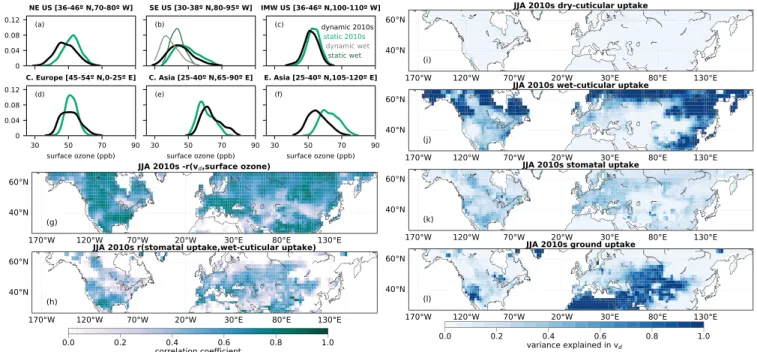
Besides summer mean differences in surface ozone between AM3DD and AM3DD-staticO3DD, there are also differences in daily probability distributions (Figures 7a–7f). For the SE United States, the distribution decreases and there are larger changes for wet days (>6 mm day−1 precipitation as defined in Travis &
Jacob, 2019) versus all days in AM3DD relative to AM3DD-staticO3DD, suggesting that high vdon rainy days
drives regional surface ozone decreases with dynamic ozone dry deposition. For the Northeast (NE) United States and the InterMountain West (IMW) United States, the mode of the distribution decreases, and the distribution shifts toward lower values. For central Asia, the mode of the distribution also decreases but the distribution shifts toward higher values. For central Europe, the distribution widens, with higher and lower surface ozone extremes.
Daily variability in vdin AM3DD may drive the changes in the distribution of surface ozone across days. However, there is some evidence that mean changes in vdmay contribute to changes in relative
variabil-ity in surface ozone. For example, reducing vdby 35% over drought-stricken regions of the eastern United
States in 1988 with the version of AM3 employing the monthly vdclimatology shifts the ozone distribution
towards higher values, but also slightly decreases the mode of the distribution (Lin et al., 2017), implying a nonlinear ozone response to a mean shift in vd. Disentangling contributions to the changes in the surface ozone distribution from daily-varying vdversus a nonlinear ozone sensitivity to vdis not possible with our
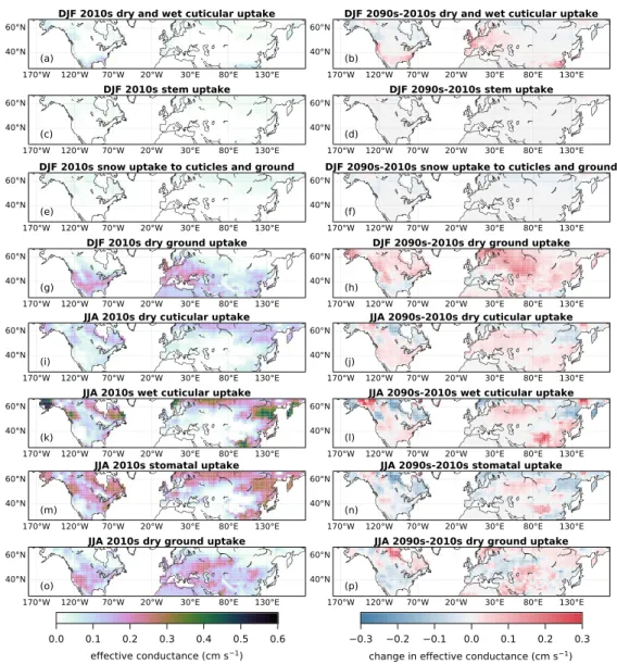
Figure 6. Winter (December–January, or DJF) and summer (June–August, or JJA) effective conductances at the 2010s,
and differences between the 2090s and 2010s under AM3DD. For a given season, we only show deposition pathways that substantially contribute to ozone deposition velocity (vd); the effective conductances shown sum to vd. The change in the effective conductances sum to the net change in vdfrom the 2010s to 2090s shown in Figure 3. For all panels, grid cells with less than 50% land are not included.
suggest that day-to-day variability in ozone dry deposition plays an important role in shaping the surface ozone distribution across days.
Kavassalis and Murphy (2017) hypothesize variability in stomatal ozone dry deposition influences daily variability in ozone pollution on the basis of the strong correlation between observed surface ozone concen-trations and vapor pressure deficit and a strong dependence of stomatal conductance on dryness. In AM3DD, nonstomatal deposition is an important fraction of the total ozone dry deposition (Figures 6i, 6k, 6m, and 6o) and a key driver of daily variability in summer vd(Figures 7i–7l), suggesting that dynamic nonstomatal
deposition also influences daily variability in surface ozone. In particular, wet cuticular and ground deposi-tion vary, reflecting the influence of soil and leaf wetness, respectively, as well as in-canopy turbulence for the latter, and dominate the variability in vdin many regions (Figures 7i–7l).
The correlation between wet cuticular and stomatal deposition (Figure 7h) and the substantial magnitude and variability that each of these terms provides summer vd(Figures 6i, 6k, 6m, 6o, and 7i–7l) imply that an unambiguous attribution of increases in ozone pollution during drought to reductions in stomatal deposition may be challenging. Lin et al. (2019) use a similar version of the GFDL model to conclude that variations in stomatal deposition drive variations in ozone pollution with drought. However, Lin et al. (2019) do not
Figure 7. Daily variability in surface ozone and ozone dry deposition. (a)–(f) Summer (June–August, or JJA) probability density functions of daily regional
average surface ozone mixing ratios for the 2010s in several northern midlatitude regions for AM3DD (dynamic) and AM3DD-staticO3DD (static) estimated with a Gaussian kernel density. For the southeast United States, we also include probability density functions for wet days only (defined as 6 mm day−1on a
regional average basis). (g) Correlation coefficient between day-to-day variability in summer surface ozone and ozone deposition velocity (vd) in AM3DD. (h) Correlation coefficient between day-to-day variability in summer effective stomatal and wet cuticular conductances in AM3DD. For panels (g) and (h), white space on land denotes correlations outside the color bar. In panel (g), all correlations shown are negative but displayed as positive. (i)–(l) Variance explained in summer daily vdby individual deposition pathways for AM3DD. We use the variance formula for variables that are not independent from each other
(Var(∑ni=1Xi) =∑ni=1Var(Xi) +2∑1≤i≤𝑗<nCov(Xi, X𝑗)) because each effective conductance is the fraction of deposition through a certain pathway multiplied by
vd. For all panels, grid cells with less than 50% land are not included.
consider how variations in cuticular uptake with precipitation influence variability in vd and thus their
conclusion may need to be revisited.
Most studies examining observed vdafter rain and dew report increases (Clifton et al., 2020). While labora-tory and field chamber evidence support increases in cuticular deposition to wet leaves (Fuentes & Gillespie, 1992; Pleijel et al., 1995; Potier et al., 2017; Sun et al., 2016), whether increases in ecosystem-scale vdafter rain
and dew are due to wet cuticular deposition is uncertain. For example, changes in other processes (e.g., stom-atal conductance, in-canopy chemistry) may contribute to observed increases (Altimir et al., 2006; Clifton et al., 2019; Turnipseed et al., 2009). Canopy interception of water is also an uncertain component of land models (Bonan & Levis, 2006; De Kauwe et al., 2013; Fan et al., 2019; Lian et al., 2018) and contributes to uncertainty in simulated wet cuticular deposition. The amount of canopy-intercepted precipitation in LM3 is lower than observation-based estimates (Milly et al., 2014) and additional uncertainty includes whether the model captures the duration and fraction of wet leaves.
In general, AM3DD may not simulate the partitioning of vdto individual pathways accurately due to
pro-cess and parameter uncertainty (e.g., m, all initial resistances). Indeed, recent work identifies factor of 2–3 differences in simulated vd due to process representation and parameter choice (Wong et al., 2019;
Wu et al., 2018). Given that AM3DD seems to capture the magnitude of vd, model LAI underestimates or
overestimates (Figure S2) may imply a nonstomatal deposition overemphasis or underemphasis, respec-tively. Comparisons with other models that prognostically simulate the components of ozone dry deposition (i.e., LAI, soil moisture) will be useful for assessing confidence in the contribution of different processes to ozone dry deposition as represented in current models.
5. 21st-Century Changes in Surface Ozone From Dynamic Ozone Dry
Deposition
5.1. Winter Northern Midlatitudes
Over northern midlatitudes, winter surface ozone increases with 21st-century reductions in anthropogenic emissions of nitrogen oxides (NOx) (i.e., 2010-to-2090 decreases of 57–69% for the highlighted regions) and
a doubling of global methane under RCP8.5 (i.e., 105% increase from 2010 to 2090) (Clifton et al., 2014; Gao et al., 2013). More specifically, reductions in regional NOx emissions under RCP8.5 over polluted midlati-tudes lead to a reversal of surface ozone seasonality from a summer to a winter peak (Clifton et al., 2014). The global methane doubling under RCP8.5 increases year-round surface ozone relative to no change in global methane, amplifying winter increases in surface ozone (Clifton et al., 2014).
We find here that increasing winter vd during the 21st-century tempers the rise in winter surface ozone
over midlatitudes in AM3DD relative to AM3DD-staticO3DD (Figures 3e, 3g, and 3i). For example, 21st-century increases in winter surface ozone are lower on average by 4–8 ppb in AM3DD relative to AM3DD-staticO3DD for highlighted regions. Over some parts of Asia, changes in local and remote ozone dry deposition tip the balance toward the 21st-century decreases in winter ozone.
Higher winter vdby the 2090s at midlatitudes (Figure 3i) mainly reflects higher ground deposition and higher dry and wet cuticular deposition (Figures 6b, 6d, 6f, and 6h). There is higher ground deposition due to less snow (not shown). Andersson and Engardt (2010) also find that decreasing snow over Europe with climate warming is an important driver of regional vdand ozone pollution for their April–October analysis. Increases in winter vdfrom higher cuticular deposition are likely associated with warmer winters and higher LAI (Figure S3) from the long-term effects of carbon dioxide fertilization (i.e., plants accumulate more biomass under high carbon dioxide).
5.2. Summer Northern Midlatitudes
Large summer decreases in surface ozone from the 2010s to the 2090s over polluted northern midlatitudes occur as regional anthropogenic NOxemissions decline under RCP8.5 (Clifton et al., 2014; Gao et al., 2013;
Rieder et al., 2018). Similar to AM3DD-staticO3DD, summer surface ozone decreases over most midlatitudes in AM3DD (Figures 3f and 3h). For highlighted regions, the 21st-century decrease in surface ozone is −7 to −17 ppb in AM3DD versus −2 to −19 ppb in AM3DD-staticO3DD; the decrease weakens by about 1 ppb in AM3DD except over central and east Asia where the decreases are the same or become stronger by 4 ppb, respectively.
Over several midlatitude regions, opposing summer changes in individual deposition pathways from the 2010s to the 2090s offset each other, leading to little net 21st-century change in vd(Figure 3j). For
exam-ple, summer dry cuticular deposition increases nearly everywhere (Figure 6j) from the long-term effects of carbon dioxide fertilization promoting leaf biomass accumulation (Figure S4a). Wet cuticular deposition increases or does not change at most midlatitudes (Figure 6l); regions with increases in wet cuticular depo-sition are regions with increases in rainfall and regions with no change are regions with decreases in rainfall (Figure S4b). Ground deposition decreases or does not change in most midlatitude regions, except western Asia (Figure 6p). Changes in ground deposition mostly reflect higher LAI (Figure S4a), which raises the resistance to in-canopy turbulence and decreases ground uptake, rather than changes in soil wetness (Figure S4d), which are mostly decreases and would lead to increases in ground uptake. Summer stomatal deposition either does not change or decreases over most midlatitude regions (Figure 6n) despite widespread increases in LAI, likely due to increased dryness (Figure S4c) and the short-term (i.e., instantaneous) effects of car-bon dioxide that induce stomatal closure. Exceptions include western Asia and the western United States, where there is vegetation at end of the century but not at the beginning (compare Figures S2b and S4a).
5.3. Summer and Winter Boreal Regions
With the prescription of land use change under RCP8.5 and the expansion of deciduous forests into boreal latitudes simulated by the vegetation dynamics in LM3, there are 21st-century decreases in winter and sum-mer cuticular deposition (Figures 6b, 6f, 6j, and 6l) over boreal regions with conifers at the 2010s. Such decreases likely occur because the model generally simulates lower LAI for deciduous forests, pastures, and crops relative to coniferous forests (not shown). There are 21st-century decreases in summer stomatal depo-sition over these boreal regions (Figure 6n), likely following decreases in LAI but also the short-term impact of high carbon dioxide. In boreal regions with deciduous forests throughout the 21st-century, increases in winter and summer vd (Figure 3i,j) follow less snow (winter only) and higher LAI from carbon dioxide
fertilization.
Our findings of mostly decreases in summer boreal vdcontrast with Wu et al. (2012) who find widespread increases in boreal summer vdbetween 2000 and 2100. Differences in vdbetween AM3DD and their model
(the dynamic vegetation model described in Sitch et al., 2003) result from different prognostically deter-mined LAI (i.e., their model shows 21st-century LAI increases over boreal regions), prescriptions of land use change, and stomatal conductance parameterizations. Wu et al. (2012) use a Jarvis (1976) stomatal con-ductance model rather than a coupled net photosynthesis-stomatal concon-ductance model as used here. While their stomatal conductance parameterization considers the long-term effect of carbon dioxide on LAI, it does not consider the short-term effect on stomatal conductance.
In general, 21st-century carbon dioxide fertilization is uncertain (Friedlingstein et al., 2006; Gerber et al., 2010; Green et al., 2019; Humphrey et al., 2018; Sulman et al., 2019; Terrer et al., 2016; Smith, Malyshev, et al., 2016; Smith, Reed, et al., 2016; Wieder et al., 2015; Yuan et al., 2019). For example, changes in other processes may offset or exacerbate the impacts of high carbon dioxide on stomatal conductance and LAI (e.g., nutrient limitation). A better understanding of carbon dioxide fertilization will lead to not only more accurate projections of stomatal deposition but also nonstomatal deposition.
6. Conclusion
Limited representation of ozone dry deposition in atmospheric chemistry models hampers understanding of ozone pollution because simulated surface ozone is sensitive to vd(Hogrefe et al., 2018; Lin et al., 2008;
Walker, 2014). Here we use a new version of the NOAA GFDL global chemistry-climate model, AM3DD, that leverages the dynamics of the underlying land model to simulate dry deposition of some aerosols and reac-tive trace gases, including ozone. Particularly novel features of the dynamic ozone dry deposition scheme are dependencies of nonstomatal deposition processes on soil moisture, canopy humidity, and canopy inter-ception of water and snow, as well as dependencies of stomatal deposition on photosynthesis, vapor pressure deficit, and soil moisture. We use this new tool to investigate the influence of ozone dry deposition on surface ozone at northern midlatitudes at the beginning and end of the 21st-century. While stomatal deposition has long been recognized as an important driver of ozone dry deposition, we show that the vdspatial distribution,
daily variability, and 21st-century changes also depend on nonstomatal deposition.
The new version of the GFDL model improves the simulation of winter ozone at surface monitoring sites and in the lower troposphere at remote sites relative to the version of the model driven with a vd
climatol-ogy. Higher simulated winter vdin AM3DD reflects our use of interactive snow dynamics and recognizing
nonnegligible winter ozone dry deposition, as supported by observations. A major finding from our study is that winter ozone dry deposition influences baseline ozone, suggesting that remote ozone dry deposition is an important lever on a given region's ozone pollution. We also find that large-scale increases in win-ter vdduring the 21st-century under RCP8.5 limit the influence of rising global methane on surface ozone (e.g., Clifton et al., 2014). For example, the change in winter surface ozone from the 2010s to 2090s with dynamic ozone dry deposition is 1 to 13 ppb over the northern midlatitude regions highlighted here versus 6 to 21 ppb with the climatology.
The dynamic ozone dry deposition scheme generally leads to −4 to +7 ppb changes in mean summer sur-face ozone at the 2010s over northern midlatitudes relative to the simulation forced with a vdclimatology. We find that daily variations in summer vdwith meteorology and biophysics, including from nonstomatal deposition processes, contribute to daily variations in ozone pollution. Evidence includes differences in daily ozone probability distributions between simulations with dynamic ozone dry deposition versus the clima-tology, daily correlations between surface ozone and vdin the dynamic simulation, and the high fraction of variance explained by nonstomatal deposition in simulated daily variations in vd. Our new dry deposition configuration supports a role for ozone dry deposition on rainy days in the pervasive summer surface ozone bias over the southeast United States. In general, simulated cuticular deposition varies similarly to stomatal deposition, suggesting unambiguous attribution of variations in vdand ozone pollution to stomatal
depo-sition may be challenging. Studies pinpointing the drivers of day-to-day variability in observed vdwill be
useful for ensuring that regional-to-global models capture the response of summer ozone dry deposition to meteorological and biophysical variability accurately.
Mostly 21st-century changes in summer surface ozone at northern midlatitudes under RCP8.5 are similar with dynamic ozone dry deposition (around 1 ppb difference). One exception is east Asia where increasing vd leads to a 4 ppb stronger decrease in summer surface ozone. In general, there are changes in summer ozone deposition pathways with changes in rainfall, dryness, and carbon dioxide. However, changes in individual pathways tend to offset one another and thus there is not much impact on the change in summer surface ozone. The extent to which this offsetting occurs, however, depends fundamentally on assumptions inher-ent to the represinher-entation of differinher-ent depositional processes in the model. Given the reliance of all ozone