Distribution Network Reconfiguration for an Apparel
Manufacturer: An Inventory Analysis
By
Pablo Tercero
BCheEng. Chemical Engineering (2001) Universidad Iberoamericana, Mexico City, Mexico
Submitted to the Engineering Systems Division in partial fulfillment of the requirements for the degree of
Master of Engineering in Logistics
at theMassachusetts Institute of Technology
June
2003
© 2003 Pablo Tercero All Rights Reserved
The author hereby grants to MIT permission to reproduce and to distr and electronic copies of this thesis document in whole or in part.
Signature of Author
Engin in Siv
Certified by
f nes aster( Executivepii ctor, Log rogram Thesis Advisor Accepted by M SSACHUSE S INSTMTUTE. OF TECHNOLOGY
JUL 27 2004
LIBRARIES
Yossi Sheffi Professor of Cix kEnviro ental Engineering Professor of Engineering Systems Co-Director, Center for Transportation and LogisticsTABLE OF CONTENTS
A BSTRA CT ... 4
1.0 IN TR O DU CTIO N ... 5
1.1 CONTEXT ... 5
1.1 IMPORTANCE OF RESEARCH ... 6
1.2 GOALS AND O BJECTIVES... 6
1.3 SCOPE OF W ORK ... 6
1.4 RESEARCH LIM ITATIONS... 7
1.5 A SSUMPTIONS ... 7
2.0 LITER A TUR E R EV IEW ... 9
2.1 THE FOOTW EAR AND A PPAREL INDUSTRY ... 12
2.2 PROJECT COMPANY ... 18
2.2.1 Production and Procurement... 19
2.2.2 Inventory Management and DC Operations... 21
2.2.3 Inbound Transportation... 23
2.2.4 Region Characteristics... 24
2.2.4.1 Region A ... 24
2.2.4.2 Region B ... 25
2.2.5 Role ofInventory... 25
2.2.6 Logistics System Costs ... 27
2.2.6.1 Fixed Costs ... 27
2.2.6.2 V ariable Costs... 28
3.0 DATA AND METHODOLOGY... 36
3.1 COMPANY D ISTRIBUTION... 36
1 .6 ... 3 6 3.2 D ATA SOURCES ... 39
3.3 INVENTORY M ODELS ... 39
3.3.1 "N ewsboy "M odel ... 39
3.3.2 Reorder Point M odel... 41
3.3.3 Quick Replenishment M odel ... 42
3.4 SAFETY STOCK... 43
3.5 ANALYSIS ... 45
3.5.1 Transportation and Labor Costs... 46
3.5.2 Inventory Impact Analysis... 47
3.5.2.1 Inventory Turns Analysis... 47
3.5.2.2 Cost Calculations ... 50
3.5.2.3 Inventory Option for Improvem ent... 62
4.0 RE SU LTS ... 71
4.1 V ARIABILITY... 71
4.2 INVENTORY TURNS RESULTS ... 73
4.3.1 R efill Inventories... 79 4.3.2 "N ew sboy " R esults ... 80 5.0 CONCLUSIONS ... 81 5 .1 O V ER V IEW ... 8 1 5.2 R ECOM M ENDATIONS ... 81 5.3 FUTURE R ESEARCH ... 82 BIBLIO G RA PH Y ... 84
APPENDIX 1: COST OF CAPITAL BY INDUSTRY... 86
APPENDIX 2: K FACTOR AND SERVICE LEVEL TABLE...88
Acknowledgments
I would like to thank
. Irene for her loving support and patience through this masters program. . Lucila, Enrique and Gonzalo for they have always been an inspiration to me. . Jonathan Fleck for his continuous support and insights in this paper.
Abstract
Companies in the footwear and apparel industry must deal with many supply chain challenges, including intense competition, long production lead times, reliance on international carriers, and shifting consumer preferences. For many large companies, only design and distribution are performed internally. This places pressure on footwear and apparel companies to continually improve supply chain management.
This study considers a company in the footwear and apparel industry and its option to consolidate distribution for two separate regions into one. One region currently serves nine times the demand of the other region. In addition, there are differences in labor and transportation costs between the two regions. The company would like to understand the financial, operational, and service impacts associated with consolidation.
This study uses a total logistics system approach with particular focus on inventory. The results indicate that if the company were to consolidate distribution for the two regions into one, then there would be a slight total logistics system cost increase. This is due mainly to differences in labor and transportation costs between the two regions. However, sensitivity analysis indicates that if some costs can be reduced, there may actually be potential savings associated with consolidating the two regions.
1.0 Introduction
1.1 Context
The recent state of the economy and progress in technology has made the search for major improvements in productivity, optimum use of financial assets, leaner operations,
and faster response to customers more important than ever. Many companies are reassessing their strategy and supply chain structure to provide growth in the long term. For example, Lucent is currently undertaking an effort to redesign its supply chain by
outsourcing non-competency functions to provide better shareholder value. See Bibliography (8).
This search for optimum use of assets generates considerable pressure on logistics networks to provide better service with minimum inventory. Companies are more interested than ever in understanding where to locate and how much inventory they should really have. After all inventory is part of a company's assets and investments and thus better management of inventory is equal to better management of assets. Inventory management is thus critical because it could reduce the capital requirements (used to buy the raw materials or the goods from the manufacturers) and allow companies to use that reduced capital to invest in other areas such as sales, marketing, or research.
1.1 Importance of Research
This thesis is concerned with inventory and other impacts of a network reconfiguration for a North American footwear and apparel company that is involved in both production and distribution of products.
The importance of this research is that companies across many industries must periodically evaluate their own networks and understand financial, operational, and service impacts of various alternatives.
1.2 Goals and Objectives
This project will analyze the financial, operational, service, and inventory impacts associated with relocating finished product inventory from one region to another. The finished product inventory is currently based in a central distribution center, but in the future it could be distributed through several category-oriented distribution centers.
1.3 Scope of Work
This project will only consider two regions of operation and two particular distribution centers for the participating company. The company's other regional and global facilities will not be considered. All variable costs for the two regions will be taken into
consideration, as well as relevant fixed costs for one region. However, the thesis project will not cover the production, inbound (ocean transportation), other distribution centers other than the two subjects of the analysis, nor the possibility of technology solutions.
Improvements or changes in other supply chain areas such as transportation, production, procurement, organizational structure, and supplier relations were out of scope.
1.4Research Limitations
Due to a limited period to collect data and ultimately complete this project, it was
necessary to use a select amount of data and interviews with key personnel. The inputs to the study were shipment data from the distribution centers, interviews with key members of the organization and a prior, related study conducted by the company.
1.5 Assumptions
In order to complete this research and analysis, it was necessary to make a number of assumptions. These include the following:
" DC shipments approximate customer demand. This is an assumption, but in reality, customer shipments can be sent incomplete.
" The data is assumed to be representative, though shipment data was used for a top selling brand that may not accurately represent other products' movements. " Lead times involved in production and procurement will remain constant and
resemble historical patterns.
" For interviews, company personnel correctly interpreted the questions and provided the answers truthfully.
- The researcher correctly interpreted the responses of supply chain managers. - The Region A facility has a capacity of 2 million units.
2.0 Literature Review
In "Quantifying the impact of inventory holding cost and reactive capacity on an apparel manufacturer's profitability," Ananth Raman and Bowon Kim, Bibliography (1) give a detailed description of a methodology to model the impact on holding costs (inventory)
for a US apparel manufacturer. Their analysis uses operations-research tools to simulate the effects of inventory holding costs on the companies over and under stocking
problems. The references in their article are mostly operations research based. As is mentioned in their article the literature regarding "fashion products " is directed towards either the manufacturer or the retailer. The company subject of the analysis has a little bit of both.
However, the article refers to a US manufacturer, with a specific model that is not suited for the business decision faced by the company in this analysis.
In terms of the decision analyzed in this thesis project, an interesting question was to see if other members of the industry were doing things similarly. In " Nike Does It," an article in Modem Materials Handling in January 2000 Bibliography (2), a description of a brand new distribution center built by the company on the title is given. The important thing to notice there is that it mentions that that company has its distribution centers divided by category, one for apparel and the other for footwear. However, it is not said why is this case or even better, if it is indeed a better DC configuration.
Inventory pooling is a subject addressed by David Simchi-Levi in Designing and Managing the Supply Chain,Bibliography(3). In this subchapter, it is described how pooling the inventory from two separate customers can reduce average inventory. It is
also mentioned there how the greater the coefficient of variation (of demand), the greater the benefit obtained from centralizing the inventory. Finally, the chapter also says that the benefits from this exercise are limited by the correlation of demand between the two regions. That is, if Region A and Region B have very similar demand patterns the
benefits of pooling are increasingly diminished. This is explained by the fact that if there is a demand peak in one market, it can be offset by a trough in the other with no DC inventory adjustment. But if the demand patterns are exactly the same, the chances for a readjustment (reordering or more system-wide inventory) are greater and the expected benefits of the project lesser. This chapter is particularly relevant to this thesis since it provides direction on the inventory impact from the distribution network reconfiguration sought by the company. It explains how average inventory has two components, of which one of them is dependent on the variability of demand (weekly, daily or yearly,
depending on the product, industry, seasonality and particularities of the company, suppliers and customers).
A good description of the manufacturer view of the supply chain is given in ""Quick Response in the Apparel Industry ", Bibliography(4), where the challenges of long lead times and the problems it causes are also treated. However the solution proposed, namely QRP adapts only to the manufacturer side, giving that type of solution to a US
The company subject to this thesis project has outsourced most of its manufacturing
activities to contractors in the Far East. This is how most footwear and apparel companies
handle operations. Bibliography(7) shows how a retailer uses this sourcing strategy for
footwear and confirms how the majority of the industry is inclined to outsourcing in the
Far East as opposed to locally.
Interesting ideas on improving the inventory problem, through better communication
systems and implementation of cross-docking operations can be found in
Bibliography(5). Although the article is almost 10 years old the ideas articulated there
still apply and are relevant to this project because the implementation of operations
similar to cross docking are one of the options considered as a solution. In this article it is
described how, Floor Ready Merchandise (FRM), which is when goods are supplied to
retailers with all necessary tags, prices, security devices already attached so that products
can move faster through retailers DC's or can be shipped directly to stores, improves the
efficiency of the logistic operation as it reduces the sometimes cumbersome and labor
intensive activities carried out in DC's to prepare the merchandise for increasingly
In the case of this project a solution similar to this could be obtained by shipping the goods out of Region A, in bulk but with quantities duly separated, and having a third party prepare the merchandise for the end customers. Anytime an additional party in this type of activity is involved ,transportation costs, along with additional handling fees for redundant activities such as loading and unloading, carton handling, etc, prohibit this type
of activity in most cases. Specific labeling activities could then be carried out in Region B more efficiently than putting away, picking back and labeling, which are time
consuming, labor intensive operations.
Another article from the same time, Bibliography(6), also points out the benefits from changing the DC to a cross docking operation. In that same tone, there is a very large base of articles pointing out the benefits of using the cross docking type of operation, some of which are mentioned in the bibliography, although as mentioned before the literature is very profuse on this subject.
2.1 The Footwear and Apparel Industry
This industry is defined generally by the following:
" Long product cycle times, 6 + months from design to manufacturing and early shipments.
- Heavy use of international sourcing and logistics " Intense competition.
This implies that companies are moving products, raw materials, work in process and finished goods through a complex logistics network. At each point in the network
inventory is generated. It is thus important to evaluate very carefully the amount and location of these assets.
The long cycle time and fragmentation of the supply chain makes planning risky and forecast errors costly. Losses within the chain come from forced markdowns due to obsolescence, stockouts and inventory carrying costs. Increases in efficiency in this intensely competitive industry are a necessity and better inventory management is one way to create them.
A prototype life cycle of a garment or pair of footwear starts in the design labs of
companies, after this design process, some samples are made and then shown to customer representatives in trade shows and other promotional events. With this information, production at large manufacturers is increased rapidly so as to meet order commitments on time. On issue is that production may take three to four months before delivery of the orders. The reasons for this long lead time vary between: the manufacturer is not
producing exclusively for one company and thus has to allocate machine and people time to fill several customer orders, procurement of large quantities of raw material such as wool and cotton takes time, however, ocean transportation, and inland haulage
(intermodal freight) are often times the more important factors. So after the samples are made and shown to potential customers, at which point the first orders are taken, the products will not be at the customers' stores until 6 months later when demand may have changed. Manufacturers and retailers share the risks of fluctuating demand in different
ways- for larger retailers the manufacturer may assume more risk in order to retain the retailer's business.
During the ordering period, there is typically a " freeze " point where the production plan becomes final, that is after that point no more orders will be generated. However, for larger customers the manufacturer may decide to take "refill " orders or smaller orders to fill unexpected or small requests from end consumers. This is typically performed with popular items that are requested by customers throughout the year.
The key insight here is that the industry commits most of its business in a make to order fashion and the rest in smaller portions because of long manufacturing and design lead times and so demand is forecasted several months in advance. A schematic ordering and production plan is shown in the next page as an example.
May'03 Jun '03 Jul'03 Aug '03 Sep'03 Oct'03 Nov'03 Dec'03 1Jan '04
ID Task Name 2 27|4 11118125 1 8 152229 6 132027 3 10172431 7 14 2128 5 12|1926 2 9 16|2330 7 14|21 2 4 11|18
1 Single Period Product Life Cycle
2 Design Process
3 Samples Production
4 Trade Show, Promotion Events 5 Feedback process
6 Other Preproduction Activities
7 Production Order Start 10/3
8 Production Process
9 Final Orders 12/26
Another characteristic of this industry is that most of the apparel and footwear is
manufactured outside the United States, the Far East holding a majority percentage of the manufacturing share both in apparel and footwear. Even though technology
improvements have helped the textiles industry to reduce the impact of labor in the cost equation, the apparel and footwear industries still require considerable, labor-intensive activities. It is generally accepted that the most cost efficient supply chain is
characterized by production in the lowest cost location, please refer to the following graph for the percentages by country of origin.
80.0% -70.0% -60.0% -50.0% 40.0% - 30.0%- 20.0%-10.0% -0.0%
2001 Percent Share of Total U.S. Footwear Imports By Country of Origin 78.8% 5.5% 4.2% 2.7% 1.7% 1.5% 0.8% 0.6% 0.6% 0.5% +c 0 %~w
Graph 1. From "Shoestats "American Apparel & Footwear Association, 2002 I
Expenditures on personal consumption in apparel and footwear have been increasing at a
slow yet steady pace for a 10-year period as shown in the graph below:
Personal Consumption Expenditures on Footwear in the US $50 4 46 47 3436 $37 ;39 U4 ~464 0 $30 S$20$1 $$10 $0
Graph 2. Source "Trends "American Apparel & Footwear Association 2001
However, the percentage of consumption in footwear from the total consumption
expenditures in the US has been deceasing also at a steady rate. (Graph 4)
085% FootwearExpenditures as a Percentage of Total Personal Consumption Expenditures (PCE)
0.80% -- " 0.75% 0.70%- 0.85%- 0.80%-1990 1991 1992 1993 1994 1995 1998 1997 1998 1999 2000 2001 -+Foo % of Tota PCE
2.2 Project Company
Before going into the analysis, it is important to present certain characteristics of the
company. These characteristics will affect the way the inventory problem is approached
and they are as follows:
. Seasonality of the industry such as the "Back to School" season.
. Cultural decisions within the company: the company is not looking at a system
wide optimization where the creation of new or leasing of existing DC's is to be
reassessed. Commercial software is readily available that can tell companies
where to locate and what sizes should the facilities be. However this is a company
centered in the New England area and because of cultural background (the
company was founded there) and of recent purchases and new lease terms of
facilities (including the general offices), it has no apparent intention in relocating
elsewhere.
. The company manages several categories of inventory, labeled activity codes.
These provide an indication of the type of movement of the product as well as the
status of its pricing. The company distinguishes two main type of products:
o Core products: these products have been a constant success across the
years, they are strong selling products that ordered every season, year
in, year out.
o In - season products: these are products that were recently introduced into the market.
In addition to categorizing by type of product, the activity also provides an indication of its pricing status. This means that if the product is no longer "in season" either because a new wave of products has been introduced and this particular product is forced out of the in season category to provide room for the new line, or because it wasn't as successful as expected and thus the company no longer considers it "in season," the product is assigned a new activity code such as "discounted". The complication in terms of inventory then comes from the fact that demand patterns for in season and core products, and of course discounted products are very different and vary within the year seasons, thus inventory decisions must take into account the different variability of the different demand patterns.
2.2.1 Production and Procurement
As explained above in the introduction there is an important differentiation made by the company in terms of its products, the seasonal and the yearlong products. The products that are "in season" or the items that are popular with customers and retailers are ordered close to 6 months in advance every month, so if the retailer wants its product on January 1st, the product is ordered to the manufacturer by mid July and shipped from the Far East in CL (full container loads) to a port.
Every month, in Region B, the customer service department analysts and managers meet to analyze a report that contains data of the inventory on hand (in the DC), inventory in transit (on their way from the Far East) and orders from customers and from this data determine the amount to be purchased. It is common practice for large manufacturers to have a minimum order size to obtain economies of scale from their facilities, this is also the case in this industry and thus customer service, in these meetings, decides either to call the customer and ask for a delay or wait until the next month, hoping that by then a minimum will be attained and a factory order can be processed.
For the sample selected for this analysis, the factory orders for that brand are sent to the offices in Region A to be consolidated. However, the Region B specific CL's are prepared and sent directly to Region B's port. From the port, a transportation third party contractor is selected to haul the finished goods to the DC.
2.2.2 Inventory Management and DC Operations
Due to the seasonal nature of the apparel and footwear business model the facility in
Region B uses a flexible labor force, with a variable working staff of around 40 people.
The distribution center has every normal put -away and picking operations observed at
any such facility with the addition of a Warehouse Management System (WMS) that
allows visibility of inventory. The main function of this system is to allocate the
incoming product and decide which product from which rack to pick. The DC personnel
use bar coding technology to tell the WMS that product has arrived, put away and picked
from the different positions inside the facility.
In terms of how much inventory is held at the DC, this is a decision driven by demand
and made by the customer service department after looking at incoming orders. For the
"in season" products, those sold for one season, the only inventory held by the company
is the pipeline inventory, meaning the 6-month pre-ordered product.
The popular products, carried out throughout the year, and even new products for which
there is indication that they could be very successful, represent 80 % of the company's
business for the brand selected for the analysis and are managed differently than the one
season only products. Although there are spikes of demand (6 months pre order) each
season, there are "refill" orders each month or week from customers that have sold their
In order to cover this more stable, yet random demand, customer service allows an excess
inventory or safety stock of 10 to 20 % of the 6-month order. It is precisely this type of
safety stock, the excess inventory, that is the key to the overall system improvement, and
thus to the savings from this project, by pooling it with the Region A's safety stock and
thus reducing the overall variability.
In the theoretical side, and as a more intuitive view of the improvement, if the regions are
different enough, any amount that a customer orders in excess of the 6 month order could
be offset by a lesser amount ordered by a customer on the other region, thus reducing the
need for both safety stocks. On the other hand the company might decide to keep both
safety stocks at one of the location and provide better service or fill rate. The reason
behind this is that because there are more inventories in the system more orders could be
satisfied from that combined pool.
The industry is intensely competitive; a failure to compete effectively could adversely
affect the market position of the company. Two of the most important areas of
competition in the industry are customer service and the ability to meet delivery
commitments to their customers. Both of these are impacted by the decision considered in
this study. As mentioned in the previous chapter service levels, because they are so
important for maintaining market share, may be set at a higher level than would be
2.2.3 Inbound Transportation
The company places orders to a number of manufacturers situated in the Far East, as
mentioned in previous subchapters, the more important ones are located in China. Once
the orders are ready to shipped, a transportation broker arranges for ocean transportation,
in general, in full ocean containers. The orders for the different regions are directed to the
company's regional ports.
Currently, the company pays different freight rates for the two regions in this study:
Company Freight Rate, Region A vs Region B
(
disguised) 3500 .c 3000 . 2500-o 2000 m Region B 1500 m Region A S1000 ~500 0
Graph 4. Source: Company's Customs and Traffic Department, Region B (disguised numbers)
In a limited number of instances, due to unexpected shifts in demand, the products are sent to designate locations as airfreight. The cost of airfreight is considerably higher than
ocean freight and thus the company focuses efforts and resources in avoiding these types
2.2.4 Region Characteristics
The differences between Region A and Region B start at this point where many
customers (almost 50 % of them) in region A receive the containers directly from the
port, the rest is sent to the product specific warehouses and then on to specific customers.
In Region B however most of the customers (approximately 90 %) do not use this policy
because their orders are not large enough to move by full container loads.
There are also differences between customers across the two regions: Region A includes
more large sized retailers such as Zellers or Foot Locker, while Region B has a higher
proportion of "moms and pops" stores (i.e. smaller). The top 20 accounts in Region B
represent 30% of that region's business.
2.2.4.1 Region A
This is the larger of the two regions considered in the project. The apparel and footwear
industry in this region is intensely competitive. The number of suppliers to the members
of the industry and especially customers is considerably bigger than in region B. The
relative buying power of customers is higher than in the other region, largely due to their
size. The size of some of these customers allows them to receive product directly from
the ports. They enjoy the economies of scale that allow them to have technology and
labor capabilities to handle the inventory at the container level. The company enjoys a
There is a distribution center for each brand managed by the company. This is consistent with what the industry in general practices.
2.2.4.2 Region B
In this region the company has only one distribution center that manages every brand that the company owns. This is possible because the demand for those products is smaller (8 to 10 % of Region A). The vast majority of the customers in this region prefer to have the company handle their inventory for them. This means that direct shipments, also called drop shipments, to the retailers are less than 3 % of the company's total shipments. An important feature of this region is that there are two official languages which implies special logistics services such as bilingual ticketing
2.2.5 Role of Inventory
Manufacturing and distribution companies often hold inventory in advance of demand. It is held on a temporary basis and is constantly being depleted, reordered and restocked .It is important to note that inventory serves different purposes:
- Process Time Inventory is required when there are long lead times between supply, manufacturing and or distribution. These delays in obtaining the inventory or shipping the goods to customers force companies to stock product in order to timely satisfy demand.
- Process Uncoupling Inventory arises when there is a need to decouple processes that benefit from economies of scale, like manufacturing (e.g. table salt) from processes that are not, such as low volume sales (e.g. sales of refrigerators). In the
examples mentioned one would like to have economies of scale manufacturing the appliances but one knows that sales of refrigerators will not sell at the same pace as they were manufactured, thus an inventory stock will be created between these two points in the supply chain.
The other reason to have uncoupling inventory is to separate supply from demand. Supply may be able and often will want to proceed at a steady, constant rate (thus eliminating costly start ups of machines) but demand is generally highly random. The solution is to have inventory as a buffer between these two processes. - Anticipation and Speculative Inventory. In this case, a company may decide to
have inventory in order to timely supply provoked demand such as a price discount promotion or to have inventory in anticipation of cost increases in raw materials.
In any case inventory serves a purpose for a company and has become an important tool for companies' supply chains. Different industries have different levels of inventory depending on the product life cycle and value. The following table provides a comparison of inventories as a percentage of total assets and of current assets (which provides a measure of what the company intends to turn into cash in the short term).
Company Inventory / Total Inventory / Current
CompanyAssets Assets
General Electric .02 .07
Tommy Hilfiger (Clothing Retail) .09 .26
Yahoo .00 .00
Wendy's .02 .13
Inventory has also become a highly visible item in companies' performance reviews because it is an explicit item in corporations' financial statements. Stockholders are interested in future sales, profits and dividends that are all related to the demand for inventory and inventory is also used as a measure of a company to continue as growing concern. Companies' creditors are also interested in inventory because they can evaluate companies' ability to turn inventory into cash that can be used to pay interests, as well as because they can hold inventory as collateral for loans.
2.2.6 Logistics System Costs
All logistics systems are composed of two types of costs: fixed and variable. These are detailed below.
2.2.6.1 Fixed Costs
These costs refer to costs that are independent of the number of units in the system. Fixed costs are incurred even if no product is bought, moved, stored, or sold. The fixed costs in this project are also termed "storage costs" that include the following:
- Cost of the lease of the facility - Utilities
- Real estate tax, " Building maintenance, - Building security,
- Insurance (for inventory and property) " Depreciation
All of which are mostly one timesaving in case the facility is removed from the
company's assets. These costs are not dependent on the number of units that the facility processes. So if it is the case that the company decides to shift only part of the volume handled by this facility to the other region, these costs will still be present and thus the savings from the project would be severely impacted.
2.2.6.2 Variable Costs
2.2.6.2.1 Transportation
Another issue to consider is the change in transportation costs whenever a centralized system is chosen over a decentralized one. The end customers for Region B will be further away from the centralized facility and so additional transportation costs will be incurred.
In the case of this project, both regions present populations that are spread out in a vast area and thus getting the product to the farthest regions may require 4 to 6 days. This is different from a project considering the same reconfiguration in a much more compact region, for example in Western Europe where distances are not such an issue.
The location of the facility is key in reducing the effects of lengthy trajectories.
Whenever one wants to minimize the transportation costs, one has to look at locating the DC at a point where distances from DC to customer are shorter than at any other point. Many commercial software solutions are available that deal with this problem using, in general, a mixed integer linear programming (MILP) optimizer. Companies like
INSIGHT, MANUGISTICS and 12 TECHNOLOGIES offer a variety of software
solutions that can accomplish these tasks. A directory of logistics software can be found at: www.goldensegroupinc.com/gateway/tech-logistics.shtml
An example of a problem formulation for the situation where transportation and operational costs are to be minimized and the optimum location or existing DC is to be chosen from the MILP:
Problem Formulation:
The problem we are facing is comparing the actual situation, servicing every customer in Region B from the Region B DC facility, to the potential optimum solution of servicing the Region B customers from existing DC'S across Region A (excluding the Region Bfor productivity and savings opportunities).
Situation Now:
The costs now are the sum of the costs of transporting every Region B DC served (CDCS) product times the quantity that is shipped to each customer reception center:
XC, +CFc
(1) Where Xi is the quantity ofproduct i shipped to its current customer reception center, Ci is the transportation cost from the DC in Region B to the customer and CFc is the cost of operating the Region B DC.
To arrive at the solution we could formulate it as a MILP problem with the following objective formula:
X X, xC,+Z xAC, xX 1
Minimize 1 (2)
Where
Xql is the quantity ofproduct i sent from DCj to customer L.
Cyjl is the cost of sending product ifrom DCj to customer 1 Zj is a binary variable, 1 ifDCj is used and 0 if it isn't.
AC] is the additional cost of operating DC with the additional load of
Xij quantity ofproduct i handled by facilityj.
Subject to certain constraints like the total demand should be filled with the DCj's (existing facilities), the capacity constraints of the existing facilities, etc.
A more detailed example can be found in Bibliography (10) where a case study with DEC is provided, the mathematical modeling is presented in the Appendix A, and (11).
However in the case of this study, the company has an arrangement with its customer in which the latter are responsible for the transportation of the goods from the companies distribution centers to their own facilities, be that other distribution centers, cross docking points or even directly to stores.
Because of this situation the analysis will focus its attention to overall inventory
reduction since this is an area where considerable savings may be derived. The additional transportation costs will be evaluated so as to understand the impact to the customers although it is a project assumption that the customer will comply with the new network requirements.
In the transportation area, the costs reported in the study that the company performed refers to:
. In the Region A case, the inbound cost for bringing the product from the Region A port and then to the Region A facility via intermodal transportation. The outbound case was considered as going from Region A to Region B in trucks.
. The Region B case refers to the actual costs incurred by the company as of today.
2.2.6.2.2 Material Handling
One other factor in the savings and opportunities analysis comes from analyzing the
operating costs related to material handling. The reasoning is as follows, since the
facilities in region A or inside region will be handling additional volume for the Region B
market, some operating costs are bound to increase, that is, because the people and assets
in these facilities will be handling more product, an analysis of the cost impact of such a
change is necessary. One approach is to multiply the costs per unit handled in each
facility (could be different for each distribution center) by the new number of units
handled by that particular facility.
In region B or outside region, the facility will not be required with the new configuration
or at the very least it will reduced its labor force so that it handles only a small number of
SKU's. In addition to this last situation is that perhaps some customer service activities
will still take place in the region B distribution center as some customizing activities will
still be required because of region B regulations, language differences and customer
knowledge and relationship.
This customization and handling of special situations (special labeling for larger
customers or promotional inserts) must be a source of attention. Customers are becoming
more and more demanding; they want an increasing number of value added activities to
On the other side there are special requirements imposed to manufacturers and retailers by governments such as labeling in different languages if the country has more than one official language (example: Belgium). These special handling activities are and additional burden to logistic facilities, which translates to extra labor, costs.
Labor availability and costs are a factor in evaluating the type of reconfiguration
analyzed in this thesis project. Different things affect labor availability and costs such as location of the facility (low population, rural areas tend to have less skilled labor).
However, of the two factors, in this case, costs is the more important one as availability is not considered an issue in Region B nor in Region A. Labor costs however are different in the two regions and they play an important role in the cost equation.
Import / export related activities such as dealing with government agencies, custom brokers and transportation contractors are also a part of operating costs in this network reconfiguration since at some point they will require people from the company to deal with them. Because the governments in the different regions have specific and often
complex import / export requirements, such as statements in different official languages, they require a special expertise. The customs department in the company has attained this expertise and is knowledgeable of the special issues that arise in the trading operations and are comfortable solving such issues. Similar expertise is required in relationships with brokers and contractors. When considering the reconfiguration like the one the company is analyzing these expert positions must receive special attention. The value of
the knowledge acquired either through formal training (in customs procedures for
example) or informal (through years of experience) are often under valued by companies.
Currently traffic or customer service departments within the logistics area handle these activities, where customs and traffic knowledgeable people have the expertise some times even, local expertise to adequately resolve the complicated day to day issues generated by the import/export matters.
Although the scope of this analysis is based on inventory impact, these operating costs related items: special services, labor availability and import/export activities should be a part of a more detailed in depth analysis.
In the labor area, the study conducted by the company included: . Payroll
. Overtime
. Benefits and Flexible benefits (given to flexible man power or contractors)
This analysis of labor was done in detail and looking at the different activities by required by the DC such as:
. Picking . Receiving
. Returns handling or reverse logistics activities. . Material handling
. Equipment maintenance . Packing
2.2.6.2.3 Holding Cost
The holding costs refer to the costs incurred when holding inventory for a period of time, this is determined not only by the quantity of inventory the company decides to hold but of the cost of capital, or the cost of investing on inventory as opposed to investing in projects or other types of investments such as securities (bonds, companies stock). This important measure is available for the apparel and shoe industries, and others, in Appendix A.
3.0 Data and Methodology
1.63.1 Company Distribution
The current company distribution network is set up as follows:
COMPANY'S NETWORK DIAGRAM
REGION B
Customer.',smm
Warehouse
Products A, B , C a
RE ' wro Oguct B
Warehouse Csoes Warehouse
Product C Product A
MMUFACTUI
The proposed change in configuration is represented below:
COMPANY'S ALTERNATIVE NETWORK
REGION B Customers wre oduct B wa a s Customers w Product C Product A REGION AWaarehouseAn alternate proposition is also being considered by this project that collects the
inventory benefits while minimizing the transportation impact, the schematic below
Company's Second Alternative Network
REGION B Customers De- Consolidation Facility Product Bother point in the network.
The main savings and opportunities as well as risks will come from 3 different sources:
3.2 Data Sources
The Information Systems department provided 78 weeks of shipment data on a weekly and monthly basis from the company's database.
Also, the researcher visited both the Region A and Region B distribution facilities.
Finally, a series of interviews were performed with supply chain managers and executives in order to understand the company's operations and processes. The Vice President of Global Logistics provided insight into the vision of the company, the overall
objective of the project as well as a description of the network and the particularities of each region. Several directors of engineering through planning were also interviewed to understand the processes of planning, overall SKU handling, the impact of seasonality.
3.3 Inventory Models 3.3.1 "Newsboy " Model
As mentioned earlier, the footwear and apparel industry is highly seasonal. This means that the normality assumption in a year time frame may be erroneous, since several seasons and thus peaks of demand occur during the year. Another possible inventory model could be the "Newsboy" in which the company has to make a one time buy and determine the appropriate level of inventory depending on the expected revenue of profit which in turn come from the probability of successfully selling a certain quantity, while considering the salvage value (discounted sale, at a loss) of that particular product.
In order to be clearer about the Newsboy model, a brief explanation is given below:
In the logistics and inventory literature, when the decision of inventory is limited to a
single time period, the problem is often referred to as the Newsboy or "Christmas Tree"
models because these scenarios are a clear example of this single time period inventory
decision. To give an example, the reader can imagine a newspaper vendor who faces the
decision each day of how many papers to buy, once he decides the quantity he cannot
back up from the decision and whatever quantity is unsold at the end of the day, will be
disposed off at a loss and this will reduce the profits of that day. It is thus in his best
interest to carefully select the one time (each day) inventory quantity. The same
reasoning applies for the Christmas trees example where at the end of the Christmas
season, each excess tree will be disposed off at a loss, diminishing the profits obtained
during the selling season.
This type of situation often arises in the style goods or fashion goods, seasonal goods and
short useful life products. The problem is then that inventory must be ordered in advance
of random demand and that any unmet demand or excess inventory will cause a cost
increase or a lesser profit respectively.
Usually demand can be forecasted by looking at historical data, however this forecast will
have an important subjective nature in that for example for new products one can only
approximate historical data because the new product is expected to generate a new
The solution to this problem comes by assuming that demand is well approximated by a discrete random variable drawn from a known probability distribution. Then the objective is to optimize the expected total revenue which is the expected revenue from sales
(demand met) plus the expected revenue from sales at salvage value (clearing of excess inventory) less the cost of the units ordered, be that newspapers, Christmas trees or fashion goods. For a more detailed discussion of this subject, see Bibliography (9)
This model may be appropriate in the case of new products, which are being introduced to the market, or "in - season " as mentioned at the beginning of the chapter. On the other hand the "core " products may be better modeled with the reorder point model.
3.3.2 Reorder Point Model
The following graph shows a schematic inventory movement in the DC's for the Reorder Point inventory model:
Inventory Flow 16000 14000- -k 12000 --- -10000 8000 --- - -6000 -2000 -_ _ __ _ _ _ __----_ _ _ __ _ _ _ __ _ _ _ __ _ _ _ 0 Weeks
3.3.3 Quick Replenishment Model
Another inventory model that could also be considered in this exercise is the pipeline model. In this model, frequent (often daily) replenishment actions coupled with long replenishment lead times (as mentioned before in this industry it could be over 6 months because manufacturing overseas), generate multiple simultaneous outstanding
replenishment orders in a pipeline of ordered product on its way to the distribution center.
The replenishment action mentioned above comes from the fact that individual customers purchase the apparel item they want at a random pace and the retailer in its effort to have better asset utilization handles little inventory and thus orders the product continuously as those individual customers remove the items from the shelf in a Quick Replenishment fashion.
In a Quick Replenishment environment retailers will replenish quantities of individual SKU's as actual sales occur. Such frequent replenishment actions, together with medium to long replenishment lead times will generate multiple, simultaneous orders, meaning a pipeline of products between the supplier's supplier and the retailer. The key decision here is what the stocking objective should be for each individual SKU.
If the variability is reduced by aggregation then less safety stock could be held within the system, providing the above mentioned possible savings. In the analysis part of this
project we will consider this demand information (shipments) to evaluate the change in
variability. Using the inventory model that best fits the company's operations choosing
from the ones mentioned above will, also provide an assessment of the potential savings
by using the inventory model that best fits the company's operations choosing from the ones mentioned above.
3.4 Safety Stock
Since the demand for products in the Region B market will be aggregated with the
demand for Region A market products there is a possible decrease in safety stock for the
aggregated or centralized system.
This is derived from the fact that the variability of the sum of the Region B demand and
the Region A demand, will be lower than the sum of the variability of each market.
Safety stock calculations use this variability number in a formula similar to: (in fact the
standard deviation is used as opposed to the variability but we know that stdev =
Jiar.)
Safety stock formula:
Equation 1
(Excluding, for the time being, lead-time and lead time variability) SLfact is a service level factor that can be obtained from tables (also called k factor), this table is provided in appendix B.
The following graphs show how the variability is reduced through aggregation
Schematic Representation of Region B demand 0.6 0.5 0.4 0.3 0.2 0.1 0
Schematic Representation of Region Ademand
0.45 0.4 0.35 0.3 - _________ 0.25 0.2 0.15 0.1 0.05
0-Schematic Representation of Aggregated Demand Region A+ Region B) 1 0.8-0.6 - - -- -0.4 -- - -0.2 0_
We can see from the graphs above that aggregating demand will reduce the variability.
This variability is directly related to the safety stock held by the facilities. So, if there is
any reduction in the variability, and hence the standard deviation by equation (1) there
will be fewer inventories in the system as a whole.
Although equation (1) may assume that demand is normally distributed (in the case
where considerable demand information, say, daily demand, can be obtained, one can use
the normal distribution assumption and its methods thanks to the central limit theorem)
and this pattern may not be exactly similar to a normal distribution, the variability
reduction leads to a reduction in inventory and thus savings because safety stock is
related to variability (or standard deviation) of demand.
3.5 Analysis
The company manages a large base of different SKUs (more than 10,000) and thus the
analysis would have been very complicated, so a sample of SKUs was made.
The sample was chosen by considering the company's business and focusing on the most
successful and largest portion of their operations. So, a special brand of footwear
products that represented 70 % of sales in 2002 was chosen. Later on a smaller segment
of SKUs within this branch of products was made through the analysis of yearly
shipments from the DC's in both regions. The end result: a selection of 138 SKUs which
Weekly shipment information for each of these SKU's (from here on in referred to as
codes) out of the Region B and Region A DC's was analyzed, finding mean and standard
deviation. The weekly demands for each code were then combined and the mean and
standard deviation for this aggregated data was obtained.
The idea behind these efforts was to find out how much the variability of demand was
reduced by aggregating it- the more different the demand patterns are between these two
locations the larger the benefits from pooling.
Of the 138 codes selected for each region, only 92 were common to both regions. A representative sample of those 92 items was selected based on the quantity shipped in
2002. For these 22 codes, the mean and standard deviation, along with those statistics for
the aggregated demand, was calculated. A summary of them for this set of data is shown
in the Results Chapter, table 4.
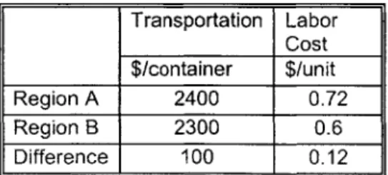
3.5.1 Transportation and Labor Costs
The table below summarizes the most important costs in the study performed by the
company, transportation includes inbound and outbound, and labor costs include all
material handling activity in the DC (picking, put away, reverse logistics, labeling).
Transportation Labor Cost $/container $/unit Region A 2400 0.72 Region B 2300 0.6 Difference 100 0.12
The longer distance that the product would have to travel drives the transportation cost difference. It is also affected by the particular rate negotiated within each region.
As mentioned before, the analysis didn't include the inventory impact. These
transportation and labor costs will be then compared to the holding and fixed costs to obtain in the end a full impact analysis of the network reconfiguration.
3.5.2 Inventory Impact Analysis 3.5.2.1 Inventory Turns Analysis
Inventory turns are an important, visible and traceable measure of the performance of a company and its ability to turn product into profits. The turns as they are described in this analysis can be obtained by dividing the shipped quantity out of the distribution centers by the average inventory held during the period those items where shipped.
The average inventory is obtained by multiplying the capacity of the DC by the
utilization of such a facility. Capacity utilization is an important measure as well, since it provides an idea of the way operations uses costly assets to provide value added for the company.
This analysis was concerned with understanding the impact in inventory of pooling the inventory used to satisfy the Region B demand with the inventory to satisfy the Region
A. One of the possible approaches is to look at the inventory turns and capacity utilization values to evaluate such an impact.
Shipments data for 2002, information of the capacity and utilization of the two involved DC's, holding costs (cost of capital, found in Appendix A for the footwear industry) and the variable cost of purchasing a unit of the company's product was obtained and used in a tool that calculates the results of the pooling of inventory.
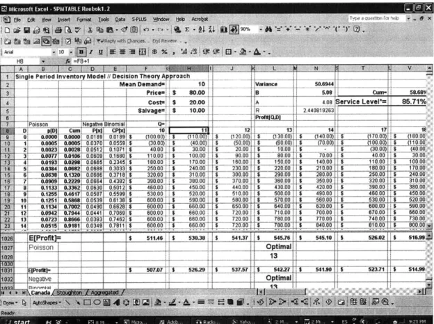
The tool takes input in certain cells (in white) and displays the results in several different spreadsheets.
Figure 1 Screenshot of the Inventory Turns tool, input page cells in white are for user input.
This tool was then used to calculate the holding, inbound, outbound, labor and fixed costs
in the current situation, the future state of the network and the difference.
For the case in which the inventories are pulled together with no other changes to the
system, that is, no improvements in the turns of the inventory, productivity or safety
stock, the facility in Region A cannot handle the new volume. It is thus assumed that the
additional volume from Region B, is absorbed by Region A in such a way that the
inventory turns in this region remain as they were prior to the addition of the new
3.5.2.2 Cost Calculations
The tool presents a spreadsheet for each of the costs involved in the project, it is
important to note that customs and ocean transportation are excluded from the analysis
since they fall outside of the scope of this project. An explanation of each cost member is
explained below.
3.5.2.2.1 Holding Costs
In this part the tool presents the average inventory held at each location as well as the
combined average inventory, which represents the case where Region B's volume is sent
to Region A. This average inventory is obtained through dividing the annual demand in
each facility by the inventory turns provided in the inputs page.
Then the value of those average inventories is calculated by multiplying them by the cost
per item, also provided in the inputs page. The days of inventory are shown as reference
and they are calculated by dividing 365 (the number of days in a year) by the inventory
turns.
The future state values of average inventory and holding costs are the next task of the
tool. The average inventory of Region A stays the same since we assumed that Region A
would continue turning inventory at 5 turns a year. Region B's average inventory
however will change since it will be turning faster than before, currently the inventory
situation: the tool calculates each facility with its volume. This value is obtained by
multiplying the value of the inventory by the cost of capital, provided in inputs.
The difference in holding costs from the current minus the future state is presented next.
It is important to be clear on what the difference means so, the following equations are
presented to improve the understanding:
Holding Cost Difference = Current Annual Holding Costs - Future State Holding Costs
3.5.2.2.2 Inbound Costs
These inbound costs represent the costs of shipping the product destined to fulfill Region B's demand, from the port to the facility, whichever that one may be. In the current situation the inbound costs are the ones incurred when bringing Region B's product to
Region B's DC. In the future state, this product will be shipped to Region A's DC.
The tool calculates the number of 40' containers, which hold approximately 6000 units each, required to move the regions demand from port to facility, by dividing Region B's
demand in pairs by 6000 units / 40' container. One of the inputs to the tool is the cost for
Region B to move such number of containers, so the freight cost or inbound cost is calculated by multiplying the number of containers by the price of freight in $ /
40'container.
The future state is obtained by multiplying that same number of containers by the freight cost in Region A. The difference of these costs defined as:
Difference in Inbound Costs = Current Inbound Costs - Future State Inbound Costs A screenshot of this page is provided below
3.5.2.2.3 Labor Impact on Region A
In this page the calculations regarding the impact of labor in Region A due to the
handling of the new volume (Region B's demand), are presented to the user.
First, Region B's current cost of handling their volume is calculated. This is
accomplished by multiplying the number of units shipped (handled) by the cost of labor
Secondly, the cost of handling that same volume in Region A is calculated by multiplying
the number of units handled in Region B by the cost of labor in $ / unit in Region A. The difference is presented at the end. The difference defined as:
Difference in Labor impact in Region A = Current Labor costs of handling - Future State Labor Costs (Region A cost of handling the Region B demand)
3.5.2.2.4 Outbound Costs
This page analyses the costs incurred by the company when Region B's demand is
shipped to that region from Region A's facility. In the current situation these outbound
costs don't exist. These are additional costs and they are calculated by assuming that the
company can send the entire Region B demand at a rate of 4, 40'containers, per week.
This would imply that the containers would be 98.6 % filled. The number of containers
per year is calculated with this assumption by multiplying 4 containers times 52 weeks.
The outbound additional cost is then calculated by multiplying that number of containers
times a fraction of the freight rate out of Region A since this considers transportation
from port to DC and the new outbound distance is only from Region A's DC to Region
B's break bulk station. In this study this freight rate was assumed to be half of Region
A's freight rate from port to DC.
3.5.2.2.5 Fixed Costs
This page presents the results of calculating the impact of the project due to fixed costs.
First the current storage costs (fixed costs) are calculated by multiplying the number of
units of Region B's demand times the storage cost, which is an input to the tool.
Then, because in the future state Region B's DC would not hold the inventory to satisfy
that regions demand, since it's being shipped from Region A, the former facility would
only need to be a portion of its current size. This reduction in size is taken as an input
the factor for future state size, then that means that in the future state Region B's facility
would be 10% of its current size.
In order to obtain the future state fixed costs, the current storage costs are multiplied by
the factor given in the inputs page. Then the difference is calculated as defined below:
Fixed Costs difference = Current Storage Costs - Future State Storage Costs
3.5.2.2.6 Labor Impact on Region B
Since, in the future state, the facility in Region B will be similar to a cross docking or
break bulking operation, the labor cost will be impacted in that region.
This page calculates such an impact by calculating the new cost of material handling in
the facility. This is obtained by multiplying the volume handled, which is Region B's
demand by the cost of labor in that region, times a factor that represents the reduction in
activities in the facility compared to the current situation that includes picking and put
away activities. This factor is an input to the tool.
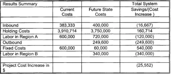
3.5.2.2.7 Results Summary
This page in the tool presents the results obtained in previous pages. The format includes
the current and future state costs as well as the difference or impact of the project. These
results are presented in the next chapter.