HAL Id: hal-01593731
https://hal.archives-ouvertes.fr/hal-01593731
Submitted on 26 Sep 2017
HAL is a multi-disciplinary open access archive for the deposit and dissemination of sci-entific research documents, whether they are pub-lished or not. The documents may come from teaching and research institutions in France or abroad, or from public or private research centers.
L’archive ouverte pluridisciplinaire HAL, est destinée au dépôt et à la diffusion de documents scientifiques de niveau recherche, publiés ou non, émanant des établissements d’enseignement et de recherche français ou étrangers, des laboratoires publics ou privés.
Mediating role of education and lifestyles in the
relationship between early-life conditions and health :
evidence from the 1958 British cohort
Sandy Tubeuf, Florence Jusot, Damien Bricard
To cite this version:
Sandy Tubeuf, Florence Jusot, Damien Bricard. Mediating role of education and lifestyles in the relationship between early-life conditions and health : evidence from the 1958 British cohort. Health Economics, Wiley, 2012, Volume 21 (Supplement S1), �10.1002/hec.2815�. �hal-01593731�
Academic Unit of
Health Economics
LEEDS INSTITUTE OF HEALTH SCIENCES
Working Paper Series No. 11_06
Mediating role of education and lifestyles in the
relationship between early-life conditions and health:
Evidence from the 1958 British cohort
Sandy Tubeuf a, Florence Jusot b, Damien Bricard c,
a
Academic Unit of Health Economics, University of Leeds, Leeds, UK
b
LEDa-LEGOS, Université Paris-Dauphine, IRDES (Institut de Recherche et de Documentation en Economie de la Santé), Paris, France
c
LEDa-LEGOS, Université Paris-Dauphine,
*
Leeds Institute of Health Sciences University of Leeds
Charles Thackrah Building 101 Clarendon Road Leeds LS2 9LJ (UK) Tel: +44 (0) 113 343 0843 Fax: +44 (0) 113 343 8496 s.tubeuf@leeds.ac.uk Disclaimer
The series enables staff and student researchers based at or affiliated with the AUHE to make recent work and work in progress available to a wider audience. The work and ideas reported here do not represent the final position and need to be treated as work in progress. The material and views expressed in the series are solely those of the authors and should not be quoted without their permission.
2
ABSTRACT
The paper focuses on the long-term effects of early-life conditions with comparison to lifestyles and current socioeconomic factors on health status in a cohort of British people born in 1958. Using the longitudinal follow-up data at age 23, 33, 42 and 46, we build a dynamic model to investigate the influence of each determinant on health and the mediating role of education and lifestyles in the relationship between early-life conditions and later health. Direct and indirect effects of early-life conditions on adult health are explored using auxiliary linear regressions of education and lifestyles and panel Probit specifications of self-assessed health with random effects addressing individual unexplained heterogeneity. Our study shows that early-life conditions are important parameters for adult health, their contribution to health disparities increases from 17.8% to 23% when mediating effects are identified. They also shape other health determinants: the contribution of lifestyles reduces from 28% down to 22% when indirect effects of early-life conditions are distinguished. Noticeably, the absence of father at the time of birth and experience of financial hardships represent the lead factors for direct effects on health. The absence of obesity at 16 influences health both directly and indirectly working through lifestyles.
Keywords: cohort; decomposition; early-life conditions; education; lifestyles Codes JEL: D63; I12.
Acknowledgements
We gratefully acknowledge financial support from the Risk Foundation (Health, Risk and Insurance Chair, Allianz). Part of this work was carried out while Damien Bricard and Florence Jusot were visiting the Academic Unit of Health Economics at the University of Leeds in summer 2010 and while Sandy Tubeuf was a visiting professor at the Université Paris-Dauphine in autumn 2010. We thank colleagues from the Academic Unit of Health Economics and the Leeds Institute of Health Sciences for their helpful comments during internal seminars. We are grateful to Anne-Laure Samson, Gang Chen, Brenda Gannon, Christine Le Clainche, and participants to the JESF 2010, the LEDA-LEGOS seminar, the Second Australasian Workshop on Econometrics and Health Economics, the CORE workshop on Equity in Health, and the JMA 2011 for useful comments and suggestions. The National Child Development Study data were supplied by the UK Data Archive (usage 54452); the authors alone are responsible for the analysis and interpretation in this paper.
1. Introduction
Numerous literature references have agreed the important role played by current individual social characteristics, such as income, education level, wealth, and social status e.g. (van Doorslaer and Koolman 2004, Cutler et al. 2006, Lantz et al. 2010) in the explanation of health inequalities. More recently, several studies have also found early-life conditions as a relevant determinant of health inequalities with a large range of social background factors, such as low parental socioeconomic status (e.g. Currie and Stabile 2003, Case et al. 2005, Lindeboom et al. 2009, Rosa-Dias 2009, Jusot et al. 2010, Trannoy et al. 2010); family issues, such as living in a single parent family or experiencing marital discord (Case and Katz 1991, Francesconi et al. 2010); parents’ health status (Trannoy et al. 2010) or health-risk lifestyles (Anda et al. 2002, Gohlmann et al. 2010, Jusot et al. 2010). However, the importance of lifestyles in the magnitude of health inequalities is less clear. Whereas epidemiological literature concluded until recently that lifestyles make a relatively minor contribution to the social gradient in health (Khang et al. 2009, Lantz et al. 2010, Skalicka et al. 2009, Van Oort et al. 2005), health economists have shown that differences in lifestyles can explain a relevant part of health and mortality inequalities (Contoyannis and Jones 2004, Häkkinen et al. 2006, Balia and Jones 2008) and a few recent epidemiological studies (Laaksonen et al. 2008, Menvielle et al. 2009, Strand and Tverdal 2004, Stringhini et al. 2010) have also confirmed that the impact of lifestyles on health and mortality disparities would be larger than it was previously estimated, particularly if lifestyles are observed longitudinally.
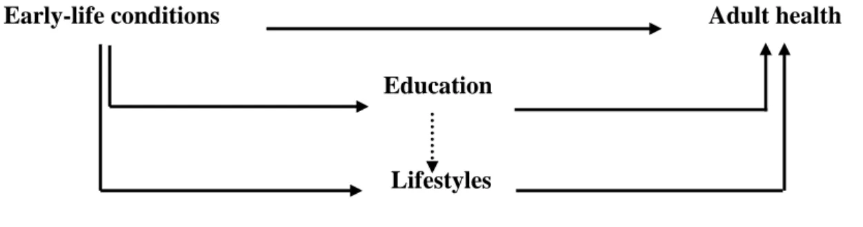
The issue at stake is that the three broad determinants of health: early-life conditions, current socioeconomic status (SES), and lifestyles cannot be considered as independent (see Figure 1). Several studies provide evidence on the transmission of SES over different generations and its relevance in the explanation of health inequalities e.g. (Marmot et al. 2001, Case et al. 2005, Trannoy et al. 2010). Moreover, parents’ characteristics and early-life conditions would also be associated
with health-related behaviours in later life (Anda et al. 2002, Rosa-Dias 2009, Gohlmann et al. 2010, Jusot et al. 2010). Similarly, several studies uncovered mechanisms through which education affects lifestyles such as obesity and exercise (Kenkel 1991, Park and Kang 2008, Webbink et al 2010), smoking (Kenkel 1991, de Walque 2007, Etilé and Jones 2010). It is therefore essential to understand the interrelationships between those various determinants of health in order to evaluate their respective contribution to the magnitude of health inequalities.
Fig. 1: Early-life conditions, socioeconomic factors, lifestyles and later-life health status
The objective of this study is to explore the long term effects of social and health-related early-life conditions, education, and early-lifestyles on health and to understand the interdependence between those three health determinants. Relying on a dynamic model of health status over the life-cycle, our empirical analysis aims to investigate the effect of each determinant in overall health inequality and determines whether early-life conditions influence health directly or indirectly, that is via affecting education and lifestyles.
Our findings provide new elements on the determinants of health inequalities which are relevant for policy makers and that remained to be empirically assessed. Firstly, the role of early-life conditions is explored in direct and indirect terms with a larger set of indicators than previous analyses, including parental social and health conditions in addition to the individual’s initial health status. Secondly, this research analyses the evolution of unhealthy lifestyles, their changes over an extended period of time and their association with health status. Finally, the longitudinal dimension of those data allows using dynamic panel analysis in order to control for unexplained individual heterogeneity and explain impact of past health status.
The structure of the paper is as follows. Section 2 describes the model that is empirically tested. Section 3 describes the National Child Development Study (NCDS) data and the variables of interest. Section 4 presents the empirical results and section 5 concludes.
2. The model
2.1 General health production function
In contrast with Jusot et al. (Jusot et al. 2010), who focused on a reduced-form model of childhood circumstances and lifestyles, we use a full model specification including individual qualification. Our approach also differs from Contoyannis and Jones (2004), Häkkinen et al. (2006), and Balia and Jones (2008), as our health production function includes early-life conditions as a potential determinant for health in addition to education and lifestyles. Furthermore, we built a dynamic model of health using longitudinal data.
The individual health status can be written using the following health production function:
(Eq. 1)
The vector of early-life conditions consists of a set of variables beyond individual control which may be related to health status. The literature on health determinants suggests an influence of childhood conditions and family background on health status in adulthood see for example Currie and Stabile 2003, Case et al. 2005, Rosa-Dias 2009, Lindeboom et al. 2009, Trannoy et al. 2010). Moreover, initial health such as birth weight and health problems during childhood and adolescence also significantly influence health in adulthood and the most adverse health risks in adulthood tend to be experienced by people having experienced poor health in childhood and adolescence (Moser et al. 2003, Case et al. 2005). The vector represents individual’s education level measured by the highest qualification achieved at age 46 and is not a time-variant variable. Researchers in many countries have found a relevant and persistent association between education and health as measured by various health measures (Grossman 2006). We assume that qualification is a reliable proxy of other social outcomes such as social class, employment status, housing or income. The vector of health-related behaviours captures individual decisions to invest in health capital, such as lifestyles (Balia and Jones 2008, Contoyannis and Jones 2004, Häkkinen et al. 2006, Rosa-Dias 2009, Jusot et al.
2010). The vector represents demographic characteristics which are biological determinants of health status, only captured by gender in cohort data. Finally, the residual term represents unobserved heterogeneity related to other random factors, which cannot be captured by observed determinants.
More concretely, let us assume that health of individual at wave is measured by a continuous latent variable which is measured using a binary variable as follows:
when
when
The general health production model can be written as follows:
with and (Eq. 2, model 1a)
We include lagged values of lifestyles into the model as past lifestyles are more likely to
be important for health status than just acquired lifestyles. The time variant individual specific error term is captured by , which is assumed to be normally distributed and uncorrelated across individuals and waves. The individual time invariant unobserved effect is captured by ; it captures unobserved individual characteristics, such as genetics and personality traits. We firstly estimate a static model with random effects assuming that the errors are independent over time and uncorrelated with the explanatory variables. This model provides us with base estimates, with which we can compare results from models that incorporate unobserved heterogeneity and state dependence.
Model 1a does not allow us to address several important issues with relevant impact on the health determinants. Firstly, we do not know whether the model variables appropriately account for any unobserved individual characteristics that also influence time-variant variables. Especially, if the past lifestyles are correlated with , we would expect to overestimate the effect of lifestyles in model 1a. Secondly, early-life conditions, education, and past lifestyles may affect current health directly but also indirectly, namely through affecting past health. If this is true, we would expect past health to influence current health, and the direct effects of early-life conditions, education, and past
lifestyles on current health to weaken or even disappear. Finally, the initial health state is likely to be not randomly assigned to the individual. To address the first issue, we use a random effect Probit specification allowing and to be correlated and introduce lifestyles averaged over time as a
set of controls for unobserved heterogeneity (Mundlak 1978). We now estimate the effects of changing lagged lifestyles on health but holding the average fixed1 in the model 1b. While this model addresses part of the problem of unobserved heterogeneity, a dynamic model of health that incorporates both past health and unobserved effects is required to address the remaining issues. The inclusion of a rich set of early-life conditions in the model can be interpreted as a particular specification of the individual component. A well-explained vector strongly contributes to the reduction of the correlation between individual effects and initial conditions as it minimises unobserved time-invariant characteristics affecting individual outcomes at each point of time. Nevertheless, we need to account the potential endogeneity bias related to the respective correlations between early-life conditions, lifestyles and education with past health, which can be ruled out using a dynamic specification and introducing past health into the health production function. The introduction of past health status in our empirical model allows us to capture the state dependence in health reports and strongly reduces the impact of individual heterogeneity. In a dynamic context, initial health is likely to be correlated with unobserved heterogeneity affecting and if
is considered exogenous this will lead to inconsistent estimators. We follow the alternative approach suggested by Wooldridge2 (2002), which requires to specify the distribution of given and
other exogenous variables and so, include at least the first value of the independent variable, .
1
Lifestyles could therefore be regarded both as a measure of lifestyles shocks on health via the past lifestyle variables and as a measure of long-term or “permanent” lifestyles on health via the average lifestyle. Nevertheless, from our point of view the follow-up of lifestyles being limited to four points of time and to the use of binary lifestyle variables does not justify to interpret the effects of lifestyles on health in terms of permanent and transitory effects.
2
Two other methods to address initial conditions problems could have been considered: Heckman (1981) and Orme (2001). The former suggests approximating the reduced form and then specifying ; is then given by integrating out (where includes all the regressors). The two main difficulties with this method are specifying the distribution of initial health, and computing time. As for Orme (2001), he suggested a two-step bias corrected procedure that is locally valid when the correlation between and is approximated to zero. A couple of recent works compared the relative performance of the three methods. Whereas Miranda (2007) concluded that the Heckman method delivers estimators that are hardly subject to bias and that are estimated with high precision; Arulampalam and Stewart (2009) concluded that none of the three estimators dominates the other two in
The ultimate latent health model that we estimate can be written as follows:
with and (Eq. 3, model 1c)
Using this dynamic model of health status over the life-cycle, we are now particularly interested in understanding the interdependent relationships linking the sets of health determinants: early-life conditions, education, and lifestyles. Therefore, we complement this primary specification with a mediating specification that aims to describe whether early-life conditions influence health directly or indirectly, that is via affecting education and lifestyles.
2.2 Mediating effects identification
The mediating specification aims to identify whether explanatory variables influence health directly or indirectly, that is by affecting or being affected by another explanatory variable. Let us firstly consider a more general case where individual health status is defined according to a set of variables , such as her early-life conditions, and a set of variables , such as her education or lifestyles.
(Eq. 4)
We consider that potentially mediates the relationship between and . For example, the early-life condition mother’s qualification may affect adult health through an effect on individual’s qualification attainment (see Figure 1) as exhibited in the pathway model that has been well-studied in both economic and epidemiological studies e.g. (Marmot et al. 2001, Case et al. 2005, Trannoy et al. 2010). We aim to evaluate the full effect of on such as follows
(Eq.5a)
However, as we are in a full model specification we cannot ignore the role played by on :
(Eq.5b)
all cases. Moreover, the authors found that it is advantageous to allow for correlated random effects using the approach of Mundlak (1978).
The total effect of on is measured by whereas the direct effect of on is measured by . The difference between and represents the mediating effects of on that work through . Moreover, the mediation effects can be written using the following auxiliary equation, where captures the effect of on :
(Eq. 6)
Using a linear model to estimate the relationship between and , we can rewrite (Eq. 5b) as follows:
= (Eq. 5c) Where represents the mediating effect, namely the indirect effect of on working through . Prior to the estimation of equation Eq. 5c, estimated residuals must be estimated from the auxiliary equations Eq. 6.
Following Bernt-Karlson et al. (2010), we can express the respective direct, mediating and total effects of on as follows:
Direct effects
Mediating effects
Total effects
Let us now consider our present study, using Figure 1, the set of variables could represent early-life conditions and the set of variables could be both education and lifestyles. In addition, the dashed arrow in Figure 1 suggests that the set of variables could represent both early-life conditions and education, and the set of variables be lifestyles only, hence there are potentially two layers of mediating effects to distinguish: mediating effects between early-life conditions and health working through education and lifestyles (mediation 1), and mediating effects between education and health working through lifestyles (mediation 2). The two different mediating specifications will be tested and compared. In concrete terms, Eq.5b corresponds to the general health production function (Eq. 3, model 1c) whereas the mediating specification is a two-step estimation based on auxiliary
equations and then the estimation of the health production function described in (Eq. 5c). The sets of auxiliary equations being estimated can be written as follows:
(Eq. 6a)
(Eq. 6b, mediation 1)
(Eq. 6b, mediation 2)
(Eq. 6c, mediation 1) (Eq. 6c, mediation 2)
If we replace those auxiliary equations into equation Eq.3, the health production function in the mediating specification becomes:
with and (Eq. 5d, mediation 1)
with and (Eq. 5d, mediation 2)
where, , , (respectively , in mediation 2) represent the estimated residuals in each auxiliary equation and can be written as follows:
(mediation 1) and (mediation 2) (mediation 1) and (mediation 2)
These estimated residuals3 are estimated as linear probability models for time-invariant outcomes and pooled linear probability models otherwise. The estimated residuals are then introduced in the health equation in replacement of the actual explanatory variables as in Eq. 5c. Using Eq. 5d, we can express the respective direct, mediating (indirect) and total effects of early-life conditions and education on health as follows:
3 For binary outcomes one estimated residual will be predicted from the OLS estimation whereas for discrete outcomes in categories, estimated residuals will be predicted corresponding to each category except the category taken as reference.
Direct effects of early-life conditions on health
Total mediating effects of early-life conditions on health
Mediating effects via education
Mediating effects via lifestyles
2.3 Health determinants decomposition
The second part of our empirical analysis inquires to which extent the account of mediating effects influences the contribution of each determinant to health disparities. Shorrocks ( 1982) showed that if we are interested in an absolute measure of inequality, i.e. a measure invariant to one translation, the variance is a good index and its natural decomposition presents the desired properties. The alternative specifications of the health production function we considered in sections 2.1 and 2.2 are based on strictly identical regressors and so, they have the same variance. The variance of both models is estimated using bootstrap method to assess variability of estimated coefficients from the panel random effect Probit (using 300 replications).
In a linear case, the share of variance explained for example by early-life conditions simply consists in the share of the of the model which is explained by . In a non linear context it is not straightforward as can only be measured as a prediction and, and are defined as independent of the set of explicative variables. A variance estimated from the data is attributed to the time invariant individual error term whereas the time variant individual error term has a
variance normalised to be equal to 1 in the case of a Probit model. We use the pseudo proposed by McKelvey and Zavoina ( 1975) in order to measure the share of variance explained by the variable having an associated coefficient , which is based on predictions of the latent endogenous variables:
(Eq. 7)
Assuming that the variance of the error term and follows a normal distribution in this
random effect Probit model, we can write:
Given the longitudinal data, the variance of the latent health variable can either be decomposed directly using the explained variance of the latent health variable, as measured by the pseudo-R2 based on all the waves. The share of inequality associated to the variable at time can thus be written as:
(Eq. 9)
3. The National Child Development Study
The National Child Development Study (NCDS) is a continuing, multi-disciplinary longitudinal study which focuses on all the people born in one week in March 1958 in England, Scotland and Wales. Information was gathered from almost 17,500 babies. Following the initial birth survey in 1958, there have been seven attempts to trace all members of the birth cohort in order to monitor their physical, educational, social and economic development. These were carried out in 1965, 1969, 1974, 1981, 1991, 1999/2000 and 2004. For the birth survey, information was obtained from the mother and from medical records by the midwife. For the purpose of the first three NCDS surveys, information was obtained from parents, head teachers and class teachers, the schools health service and the subjects themselves (who completed tests of ability and, latterly, questionnaires). In the 1981 and later surveys, information was gathered by professional survey research interviewers. In 1981 information was obtained from cohort members and from the 1971 and 1981 Censuses. In the 1991 survey there was a professional interview with the cohort member along with self-completion questionnaires from NCDS subjects and husbands, wives, and cohabiters. For the 1999-2000 sweeps, information was obtained from cohort members by interviewer and self-completion using CAPI. The 2004 survey was administered by telephone.
For the purpose of our study, we focus on the four last sweeps of the cohort (t= 0, ..., 3) in order to have repeated measures of both lifestyles and health status as an adult. Data collected before age 23 are used to inform individual early-life conditions (see in Appendix Table A.I). We have excluded cohort members who missed at least one of the four first sweeps in order to ensure a description of childhood conditions with a limited non response. The balanced sample for which individuals have fully informed health status and lifestyles in all the sweeps 4 to 7 contains 4,480 individuals whereas the unbalanced sample contains between 5,900 and 7,900 individuals. A description of the distribution of relevant variables in the balanced sample at t=0 is available in appendix (see Table A.II)
3.1.1 Health variable
The NCDS includes only one repeated measure of the respondent’s health in the cohort, namely self-assessed health (SAH). Respondents are asked to rate their own health on a four or five point categorical scale ranging from poor (sweeps 4, 5 and 6) or respectively very poor (wave 7) to excellent health status. Given the changes in scale in the variable over the different waves, we use SAH as a binary variable4 which takes the value one if the individual rates her health as good health or higher, and zero if she rates her health less than “good”. Self-assessed health has been shown to be a good predictor of mortality, morbidity and subsequent use of health care (Idler and Benyamini 1997). The distribution of health status in the balanced sample shows the age effect on health status over the life-cycle (see Table A.III). Whereas good health represents 92.7% of respondents at 23 years old, the proportion of respondents reporting a good health declines to 78.3% at 46 years old. Between the first three sweeps the mean is declining by a constant rate of 4 percentage points. There is a break with a decrease of 6 percentage points between the two last sweeps despite they are separated by four years only. This difference could be explained by an increasing effect of ageing on
4
Dichotomisation was also required as the necessary condition on the proportional odds assumption for ordinal Probit models turns out not found to be valid.
health when the cohort member enters her forties. This shift could also come from the change in the categorical scale of self-assessed health between sweep 6 and sweep 7 and this latter issue is minimised by the dichotomisation of health.
3.1.2 Socioeconomic status
The NCDS provides several current social characteristics. Education is provided at each wave and we use the highest qualification achieved over the period, generating a three categories discrete variable: having a qualification lower than O-level, having O-level or A-level, and having a qualification higher than A-level. About one fifth of respondents have a qualification lower than secondary school.
3.1.3 Lifestyles variables
The NCDS includes a longitudinal follow-up of lifestyles and health records at age 23, age 33, age 42 and age 46. We consider four lifestyles binary variables (presented in Table A.IV). Exercising indicates whether the cohort member is regularly doing exercise or sports; it equals one if the cohort member did exercise at least once in the last four weeks and zero otherwise. Non smoking informs whether the cohort member is a current smoker at the time of the wave; it equals one if she does not currently smoke and zero otherwise. Drinking prudently is a gender-specific indicator based on the number of units of alcohol drinks taken the week before the interview. Males are considered to drink prudently if they drank between 0 and 21 units of alcohol whereas it is between 0 and 14 units a week for females (Working Party of the Royal College of Physicians UK 2001, Balia and Jones 2008). The binary variable takes the value one if the respondent drinks prudently and zero otherwise. The absence of obesity is the fourth lifestyle that we consider. Obesity may appear as an intermediated or genetic outcome of health and not a pure lifestyle. Given that we can control the genetic and the family transmitted effect on obesity using the respondent’s obesity status when she was 16, the absence of obesity will thus captures aggregated effects of lifestyles. Absence of obesity
is constructed using the reported height and weight and calculating individuals’ body mass index (BMI5). The absence of obesity is a binary variable taking the value one if the cohort member’s BMI is strictly lower than 30 and zero otherwise.
3.1.4 Early-life conditions
The vector of early-life conditions that we consider has three main types of variables: social conditions in childhood, parents’ health and health-related behaviours, and child and adolescence health. Social conditions in childhood include the father’s social class at the time of birth, the father and the mother’s education level, and parental reports of financial hardships when the cohort member was 16. Father’s social class is described in three large categories: a top class (I/II) including professional and managerial or technical workers, a middle class (III) including skilled workers and armed services, and a low class (IV/V) including partly skilled and unskilled workers and a fourth category is added if the mother reported no male figure in the household at the time of birth. Parental education consists in a two categories variable: parents who dropped out from school before or at the minimum age (14-15 years depending on the year of birth) and parents who were still at school after this age. Parents’ health is measured by parental report of chronic illness when the cohort member was 16 years old. Regarding parents’ health related lifestyles, we used a smoking indicator for each parent taking the value 1 if reported to be a smoker. Respondent’s health in childhood and adolescence are used as control variables but also as achievement variables since they may represent health-related difficulties from the living environment during childhood. We use the same approach as Case et al. (2005) who considered the report of at least one chronic condition at 16 as well as a birth weight below 2.5kg as health indicators before adulthood using the same dataset. Furthermore, we include obesity at 16 years old. We have computed BMI using medical assessment
5
of height and weight and evaluated obesity level using gender-specific thresholds values found to be a good predictor of obesity at 18 (Lahti-Koski and Gill 2004).
4. Results
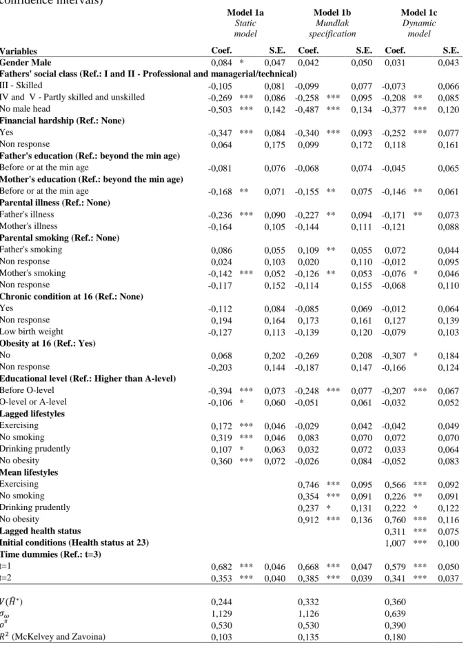
4.1 Random effect dynamic panel Probit results
The results of the random effect panel Probit of the general specification are presented in Table I. Three different models are reported: model 1a and model 1b are static models with random effect with model 1b including the average individual lifestyles over the studied period; whereas model 1c is a dynamic random effects Probit model.
Table I. Random effect Probit models results
The results show that several early-life conditions have a statistically significant effect on the probability to report good health regardless of the model. Individuals whose father belonged to the lowest social class, namely partly skilled and unskilled workers as well as individuals who had no father at the time of their birth are significantly less likely to report good health. Similarly, the experience of financial hardship during childhood has a significant and negative effect on reports of good health. The mother’s education level is also found as a statistically significant determinant of poor health reports whereas the father’s education is not significant in any of the models. This may be explained by father’s social class being significant and so, absorbing the effect of father’s education on descendant’s health. Unlike mother’s illness, father’s illness significantly reduces the probability to report good adult health. Mother’s smoking behaviour appears to be significant for descendant’s report of good health but the significant level weakens in the dynamic model. Individual education level is also found statistically and significantly associated with health: low qualification is negatively associated with the report of a good health. Regarding lifestyles variables, the four lagged lifestyles are significantly associated with reports of good health in model 1a (at the
10% level for drinking prudently). However as soon as average lifestyles are added to the model, the lagged lifestyles are not significant for health anymore. The average behaviours in exercise, absence of obesity and to a lesser extent the absence of smoking are found strongly and significantly associated with reports of good health, whereas the average behaviour towards drinking is significant at the 10% level only.
This first table of results emphasises the relevance of a dynamic model; past health status and initial health in model 1c are significantly associated with reports of good health and the share of individual unexplained heterogeneity addressed by the model equals 36% of the unexplained heterogeneity. Furthermore, when past and initial health variables are introduced a reduction in the magnitude of the model’s estimated coefficients is observed.
4.2 Auxiliary equations estimations
Prior to the mediating specification, the auxiliary equations are estimated. The results are presented in Appendix (Table A.V to Table. IX). Education is estimated as a linear regression model for the two binary variables within model 1c (having a qualification lower than O-level and having a qualification between O-level and A-level). Having a qualification lower than O-level is found positively and significantly associated with low father’s social class and absence of a male head at the time of birth, experience of financial hardship, both parents’ having left school before or at the minimum legal age and both parents’ being smokers; presence of a chronic disease at 16 years old, obesity at 16, and low birth weight. Inversely, having a qualification between O-level and A-level is found positively and significantly associated with low father’s social class, both parents’ having left school before or at the minimum legal age. On the other hand it is found negatively associated with having experienced financial hardships; mother’s smoking and having a chronic disease at 16 years old. The four lifestyles are estimated as OLS models on the pooled sample. Exercising is significantly and negatively associated with reports of chronic disease at 16, father’s low social class,
both parents’ low education and experience of financial hardship. When education is controlled (Table A.VI, column b), both low and middle qualifications are found significantly and negatively associated with regular exercise. Moreover, it weakens the significant effect of financial hardships, father’s social class and parental education. With regard to smoking behaviour, the absence of smoking is strongly and negatively associated with both parents’ smoking, financial hardship at 16, father’s low social class and the absence of male head at the time of birth. When individual education is introduced (Table A.VII, column b), both qualification lower than O-level and between O-level and A-level are found negatively correlated with the absence of smoking. Moreover, the inclusion of individual education absorbs the effect of father’s social class and weakens the impact of financial hardship. Drinking prudently is strongly higher among female and found negatively and significantly correlated with father’s smoking. Noticeably, having a father who was in lower social class and low birth weight appear to be positively associated with prudent drinking. Middle qualification is found to be negatively associated with drinking prudently when education is introduced in the auxiliary equation (Table A.VIII, column b). Finally, the absence of obesity at 16 is statistically associated with non obesity in adulthood; in addition, mother’s smoking, father’s SES and mother’s low education are found statistically significantly for the reduction of the absence of obesity. When education is included within the auxiliary equation (Table A.IX, column b), low individual education appears to be significantly and negatively associated with the absence of obesity and the introduction of individual education erases the significant effect of parents’ education which was previously observed.
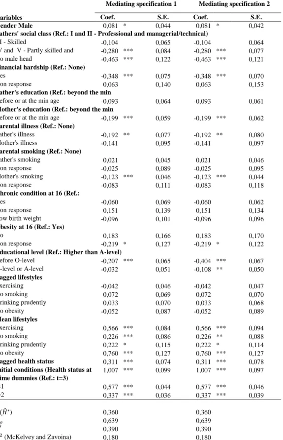
4.3 Random effect dynamic panel Probit results: mediating specification
The results of the mediating specifications of the health production function are presented in Table II. They have been obtained by replacing actual variables of education and lifestyles by the
estimated residual terms of the different auxiliary equations whose results were described in the previous section. The two mediating specifications are presented.
Table II. Random effect Probit models coefficients of the mediating specifications
Noticeably, the estimated coefficients associated to education and lifestyles in mediation 1 and to lifestyles only, in mediation 2 are strictly identical with the estimated coefficients in model 1c (see Table I) as expected when comparing Eq. 3 and Eq. 5d. The results of the mediating specification permit confirming the existence of indirect effect of early-life conditions variables on health over the life cycle in addition to their direct effect previously shown by the initial specification. There is a clear increase in the magnitude of all the estimated coefficients associated to early-life conditions in the mediating specification compared to the results of model 1c. The effect of early-life conditions is magnified when mediating effects with other health determinants such as education and lifestyles are disentangled. Moreover, this specification highlights the indirect effect of mother’s smoking status on cohort member’s health, which is found significantly associated with health in the two mediation specification but not in model (1c). The mediating specification 2 also emphasised that education level has a direct and an indirect effect on health as education as the estimated coefficients associated to the education variables are larger and the significance of having a qualification between O-level and A-level becomes statistically significant. The mediating specifications allow us to evaluate the magnitude of the direct and indirect effects of early-life conditions on adult health, working through education and lifestyles.
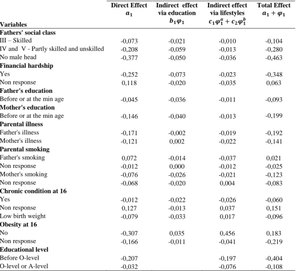
Table III presents the magnitude of direct and indirect effects of each of the variables within the vector of early-life conditions. The absence of male head at the time of birth has the highest direct effect on adult health. The experience of financial hardships during childhood is also an important early-life condition influencing adult health directly. The absence of obesity at 16 years has both relevant direct and indirect effects on adult. As an indirect effect, it essentially works
through lifestyles. The indirect effect of father’s smoking also appears to work mainly through lifestyles whereas the indirect effect of mother’s smoking works through both education and lifestyles. Noticeably, most of the indirect effects related to the father’s SES and both parents’ education level work through education. Finally, individual qualification influences health both directly and indirectly through lifestyles.
Table III. Early-life conditions direct and indirect effects on health
4.4 Decomposition of health inequality
Table IV presents the results of the decomposition of the variance of the predicted latent health within the longitudinal panel data analysis for the alternative specifications (model 1c and specification 2).
Table IV. Decomposition of health inequality (with bootstrapped 95% confidence intervals)
The decomposition in the baseline specification shows that the most important contribution to health inequalities comes from the state dependence of health and the initial health, which would explain 33.3% of the variance in the predicted health. Lifestyles are directly explaining 28.5% of health inequalities, which confirm that they are important determinants of health inequalities. Early-life conditions explain about 18% of health inequalities. If we add their indirect contributions to health inequalities, as done in the mediating specification, the relative contribution of early-life conditions increases and would represent 24% of health inequalities. This increase underlines the importance of the mediating effects of early-life conditions with education and lifestyles. On the contrary, the contribution of lifestyles on health inequalities reduces and would represent 22.2% of inequalities. Lifestyles are thus strongly influenced by early-life conditions and to a lesser extent by educational level whose contribution to health inequalities slightly increases in the mediating approach. Comparison between the decompositions of the general specification and the mediating
model suggest that the correlation between early-life conditions, and respectively lifestyles and education, is important. When we purge the contribution of lifestyles to health inequalities from their mediating effect with early-life conditions and education, we reduce their contribution to health inequalities and emphasise the importance of early-life conditions for health inequalities over the life cycle.
We thoroughly studied the share of early-life conditions in health inequalities and explore the relative contribution of social background, parent’s health and lifestyles, and initial health to this vector. The decomposition in the general specification model suggests that social background variables are the leading contributing factor, representing about 66.3% of the share of early-life conditions in health inequalities. Parent’s health and lifestyles represent about 19.3%.
5. Conclusion
In this paper, we developed a model to evaluate the contribution of several essential determinants of health to health inequalities using a representative cohort of individuals born in 1958 and a unique follow-up of health status, lifestyles as well as a good description of early-life conditions. Our results showed the indirect effects of early-life conditions variables on health over the life cycle in addition to their direct effects. Early-life conditions have a predominant contribution in health inequality when their indirect role on education achievement as an adult and lifestyles were taken into account representing 24% of overall health inequality. This latter result underlines the relevance of mediating effects between the determinants of health and outperforms previous works excluding early-life conditions as a relevant determinant of health inequalities along with socioeconomic factors and lifestyles. Among early-life conditions, social background seems to be the most important determinant of overall health inequalities. Lifestyles show an impressive contribution to health inequalities, namely 28.6%, in the general specification but appear to be determined by both early-life conditions and education, confirming previous results which have underlined social
determinism along with the existence of an accumulation of risk on causal pathways in the life course (Kuh et al. 2003).
The study exhibits among the early-life conditions those which influence adult health directly, indirectly and both directly and indirectly. The absence of father at the time of birth and experience of financial hardships represent the lead factors for direct effect on health. The absence of obesity at 16 influences health both directly and indirectly working through lifestyles. Indirect effects dramatically increase the relative contribution of early-life conditions to health inequalities, since their contribution equals 24% in the mediating model and thus becomes directly comparable to the contribution of lifestyles (22.2%).
Finally, the dynamic panel analysis permits controlling a large part of individual unexplained heterogeneity as well as the important effect of health state dependence over time. Our study has some limitations. The inequality measure is based on the explained part of the variance that is allowed by the model specifications. According to the pseudo-R² that is built using the variance of the latent variable, we would be able to explain about 18%. Therefore the unexplained health inequality remains very large. The panel data perspective also presents several limits. The first problem is the presence of attrition due to mortality in the cohort that we have ignored in the analysis. This leads us to an underestimation of the effect of early-life conditions, adult socioeconomic factors and lifestyles on health inequality as we worked on a selected sample of British people still alive at 46 years old. We did investigate mortality in our data and we found that mortality rate appears to be more important before age 23 than between age 23 and age 46. Finally, the NCDS cohort has a singular structure as the different waves are not equidistant in time. In particular there is a four year interval between the two last sweeps whereas there were about ten years between the past sweeps. We tried to catch this effect by introducing a year dummy into the
models. Therefore, the estimated coefficients in the models can be interpreted as a mean of the effects of lifestyles, education, and early-life conditions over time.
The study of the social determinants of health inequality together with lifestyles and the evaluation of their respective contribution to the magnitude of health inequality is particularly relevant for policy makers. The legitimacy of policies to tackle health inequalities is related to the relative contribution of each broad factor. Early-life conditions, which are factors that cannot be chosen by the individual, appear to be leading factors of health disparities. They are thus considered as the most illegitimate sources of health inequalities (Roemer 1998; Dworkin 1981) and would undoubtedly justify policy interventions that aim to compensate individual for inequalities of opportunity in health.
6. References
1. Anda, R. F., Whitfield, C. L., Felitti, V. J., Chapman, D., Edwards, V. j., Dube, S. R., & Williamson, D. F. 2002, "Adverse childhood experiences, alcoholic parents, and later risk of alcoholism and depression", Psychiatric Services, vol. 53, no. 8, pp. 1001-1009.
2. Arulampalam, W. & Stewart, M. B. 2009, "Simplified implementation of the Heckman estimator or the dynamic Probit model and a comparison with alternative estimators", Oxford
Bulletin of Economics and Statistics, vol. 71, no. 5, pp. 659-681.
3. Balia, S. & Jones, A. 2008, "Mortality, lifestyles and socio-economic status", Journal of Health
Economics, vol. 27, pp. 1-26.
4. Bernt Karlson, K., Holm, A., & Breen, R. 2010, "Total, Direct, and Indirect Effects in Logit Models", CSER WP no. No 005.
5. Case, A., Fertig, A., & Paxson, C. 2005, "The lasting impact of childhood health and circumstance", Journal of Health Economics, vol. 24, pp. 365-389.
6. Case, A. & Katz, L. 1991, "The company you keep: the effects of family and neighborhood on disadvantaged youths", NBER Working Paper.
7. Contoyannis, P. & Jones, A. 2004, "Socio-economic status, health and lifestyle", Journal of
Health Economics, vol. 23, pp. 965-995.
8. Currie, J. & Stabile, M. 2003, "Socioeconomic status and child health: why is the relationship stronger for older children", American Economic Review, vol. 93, no. 1813, p. 1823.
9. Cutler, D. M., Deaton, A., & Lleras-Muney, A. 2006, "The determinants of mortality", Journal
of Economic Perspectives, vol. 20, no. 3, pp. 97-120.
10. de Walque, D. 2007, "Does education affect smoking behaviors? Evidence using the Vietnam draft as an instrument for college education", Journal of Health Economics, vol. 26, no. 5, pp. 877-895.
11. Dworkin, R. 1981, "What is equality ? Part I: Equality of Welfare", Philosophy and Public
Affairs, vol. 10, pp. 185-246.
12. Etilé, F. & Jones, A. 2010, "Schooling and smoking among the Baby Boomers: an evaluation of the impact of educational expansion in France", Journal of Health Economics, vol. doi:10.1016/j.jhealeco.2011.05.002.
13. Francesconi, M., Jenkins, S. P., & Siedler, T. 2010, "The effect of lone motherhood on the smoking behavior of young adults", Health Economics, vol. 19, no. 11, pp. 1377-1384.
14. Gohlmann, S., Schmidt, C. m., & Tauchmann, H. 2010, "Smoking initiation in Germany: the role of intergenerational transmission", Health Economics, vol. 19, no. 2, pp. 227-242.
15. Grossman, M. 2006, "Education and nonmarket outcomes," in Handbook of the Economics of
Education - vol 2, Elsevier edn, E. A. Hanushek & F. Welch, eds., pp. 577-633.
16. Hakkinen, U., Jarvelin, M.-R., Rosenqvist, G., & Laitinen, J. 2006, "Health, schooling and lifestyle among young adults in Finland", Health Economics, vol. 15, no. 11, pp. 1201-1216.
17. Heckman, J. J. 1981, "The incidental parameter problem and the problem of initial conditions in estimating a discrete time-discrete data stochastic process," in Structural Analysis of Discrete
Data with Econometric Applications, Cambridge: the MIT Press edn, C. F. Manski & D. L.
McFadden, eds., pp. 179-195.
18. Idler, E. L. & Benyamini, Y. 1997, "Self-rated health and mortality: a review of twenty-seven community studies", Journal of Health and Social Behaviour, vol. 38, no. March, pp. 21-37.
19. Jusot, F., Tubeuf, S., & Trannoy, A. 2010, "Effort or circumstances: does the correlation matter for inequality of opportunity in health", Working Paper IRDES, vol. DT33.
20. Kenkel, D. S. 1991, "Health behavior, health knowledge, and schooling", The Journal of
Political Economy, vol. 99, no. 2, pp. 287-305.
21. Khang, Y.-H., Lynch, J., Yang, S., Harper, S., Yun, S.-C., Jung-Choi, K., & Kim, H. R. 2009, "The contribution of material, psychosocial, and behavioral factors in explaining educational and occupational mortality inequalities in a nationally representative sample of South Koreans: relative and absolute perspectives", Social Science and Medicine, vol. 68, no. 5, pp. 858-866.
22. Kuh, D., Ben-Shlomo, Y., Lynch, J., Hallqvist, J., & Power, C. 2003, "Life course epidemiology", Journal of Epidemiology and Community Health, vol. 57, no. 10, pp. 778-783. 23. Laaksonen, M., Talala, K., Martelin, T., Rahkonen, O., Roos, E., Helakorpi, S., Laatikainen, T., & Prattala, R. 2008, "Health behaviours as explanations for education level differences in cardiovascular and all-cause mortality: a follow-up of 60,000 men and women over 23 years",
24. Lahti-Koski, M. & Gill, T. 2004, "Defining Childhood Obesity," in Obesity in Childhood and
Adolescence, W. Kiess, C. Marcus, & M. Wabitsch, eds., pp. 1-19.
25. Lantz, P., Golberstein, E., House, J. S., & Morenoff, J. 2010, "Socioeconomic and behavioral risk factors for mortality in a national 19-year prospective study of US adults", Social Science and
Medicine, vol. 70, no. 10, pp. 1558-1566.
26. Lindeboom, M., Llena-Nozal, A., & van der Klauuw, B. 2009, "Parental education and child health: evidence from a schooling reform", Journal of Health Economics, vol. 28, no. 1, pp. 109-131. 27. Marmot, M., Shipley, M. J., Brunner, E. G., & Hemingway, H. 2001, "Relative contributions of early-life and adult socioeconomic factors to adult morbidity in the Whitehall II study", Journal of
Epidemiology and Community Health, vol. 55, no. 5, pp. 301-307.
28. McKelvey, R. D. & Zavoina, W. 1975, ""A statistical model for the analysis of ordinal level dependent variable", Journal of Mathematical Sociology, vol. 4, pp. 103-120.
29. Menvielle, G., Boshuizen, H., Kunst, A. E., Dalton, S., Vineis, P., Bergmann, M., Silke, H., Ferrari, P., Raaschou-Nielsen, O., Tjonneland, A., Kaaks, r., & et al. 2009, "The role of smoking and diet in explaining educational inequalities in lung cancer incidence", Journal of the National Cancer
Institute, vol. 101, no. 5, pp. 321-330.
30. Miranda, A. Dynamic Probit models for panel data: A comparison of three methods of estimation. 2007. United Kingdom Stata Users' Group Meetings 2007 11. Ref Type: Slide
31. Moser, K., Li, L., & Power, C. 2003, "Social inequalities in low birth weight in England and Wales: trends and implications for future population health", Journal of Epidemiology and
Community Health, vol. 57, pp. 687-691.
32. Mundlak, Y. 1978, "On the pooling of time series and cross-section data", Econometrica, vol. 46, no. 1, pp. 69-85.
33. Orme, C. 2001, "Two-step inference in dynamic non-linear panel data models", Mimeo no. Revision of Economics Discussion Paper 9633: "The initial conditions problem and two-step estimation in discrete panel data models".
34. Park, C. & Kang, C. 2008, "Does education influence healthy lifestyles?", Journal of Health
Economics, vol. 27, no. 6, pp. 1516-1531.
35. Roemer, J. 1998, Equality of opportunity, Harvard University Press edn, Cambridge.
36. Rosa-Dias, P. 2009, "Inequality of Opportunities in Health: Evidence from a UK cohort study",
Health Economics, vol. 18, no. 9, pp. 1057-1074.
37. Shorrocks, A. 1982, "Inequality Decomposition by Factor Components", Econometrica, vol. 50, no. 1, pp. 193-211.
38. Skalicka, V., van Lenthe, F., Bambra, C., Krokstad, S., & Mackenbach, J. P. 2009, "Material, psychological, behavioural and biomedical factors in the explanation of relative socio-economic inequalities in mortality: evidence from the HUNT study", International Journal of Epidemiology, vol. 38, no. 5, pp. 1272-1284.
39. Strand, B. H. & Tverdal, A. 2004, "Can cardiovascular risk factors and lifestyle explain the educational inequalities in mortality from ischaemic heart disease and from other heart diseases? 26 year follow up of 50 000 Norwegian men and women", Journal of Epidemiology and Community
Health, vol. 58, no. 8, pp. 705-709.
40. Stringhini, S., Sabia, S., Shipley, M. J., Brunner, E. G., Nabi, H., Kivimaki, M., & Singh-Manoux, A. 2010, "Association of socioeconomic position with health behaviors and mortality", The
Journal of the American Medical Association, vol. 303, no. 12, pp. 1159-1166.
41. Trannoy, A., Tubeuf, S., Jusot, F., & Devaux, M. 2010, "Inequality of Opportunities in Health in France: A first pass", Health Economics, vol. 19, no. 8, pp. 921-938.
42. van Doorslaer, E. & Koolman, X. 2004, "Explaining the differences in income-related health inequalities across European countries", Health Economics, vol. 13, no. 7, pp. 609-628.
43. Van Oort, F., van Lenthe, F., & Mackenbach, J. P. 2005, "Material, psychosocial, and behavioural factors in the explanation of educational inequalities in mortality in the Netherlands",
Journal of Epidemiology and Community Health, vol. 59, no. 3, pp. 214-220.
44. Webbink, D., Martin, N. G., & Visscher, P. M. 2010, "Does education reduce the probability of being overweight?", Journal of Health Economics, vol. 29, no. 1, pp. 29-38.
45. Wooldridge, J. 2002, Econometric Analysis of Cross Section and Panel Data, MIT Press edn, Cambridge.
46. Working Party of the Royal College of Physicians UK 2001, Alcohol - Can the NHS afford it?
Recommendations for a coherent alcohol strategy for hospitals, NHS edn, London.
7. Figures
Fig. 1 Early-life conditions, socioeconomic factors, lifestyles and later-life health status
8. Tables
Adult health
Lifestyles Education Early-life conditions
Table I. Random effect Probit models results with estimated coefficients (with bootstrapped 95% confidence intervals) Model 1a Static model Model 1b Mundlak specification Model 1c Dynamic model
Variables Coef. S.E. Coef. S.E. Coef. S.E.
Gender Male 0,084 * 0,047 0,042 0,050 0,031 0,043
Fathers' social class (Ref.: I and II - Professional and managerial/technical)
III - Skilled -0,105 0,081 -0,099 0,077 -0,073 0,066 IV and V - Partly skilled and unskilled -0,269 *** 0,086 -0,258 *** 0,095 -0,208 ** 0,085 No male head -0,503 *** 0,142 -0,487 *** 0,134 -0,377 *** 0,120 Financial hardship (Ref.: None)
Yes -0,347 *** 0,084 -0,340 *** 0,093 -0,252 *** 0,077 Non response 0,064 0,175 0,099 0,172 0,118 0,161 Father's education (Ref.: beyond the min age)
Before or at the min age -0,081 0,076 -0,068 0,074 -0,045 0,065 Mother's education (Ref.: beyond the min age)
Before or at the min age -0,168 ** 0,071 -0,155 ** 0,075 -0,146 ** 0,061 Parental illness (Ref.: None)
Father's illness -0,236 *** 0,090 -0,227 ** 0,094 -0,171 ** 0,073 Mother's illness -0,164 0,105 -0,144 0,111 -0,121 0,088 Parental smoking (Ref.: None)
Father's smoking 0,086 0,055 0,109 ** 0,055 0,072 0,044 Non response 0,024 0,103 0,020 0,110 -0,012 0,095 Mother's smoking -0,142 *** 0,052 -0,126 ** 0,053 -0,076 * 0,046 Non response -0,117 0,152 -0,114 0,155 -0,068 0,110 Chronic condition at 16 (Ref.: None)
Yes -0,112 0,084 -0,085 0,069 -0,012 0,064
Non response 0,194 0,164 0,173 0,161 0,127 0,139 Low birth weight -0,127 0,113 -0,139 0,120 -0,079 0,103 Obesity at 16 (Ref.: Yes)
No 0,068 0,202 -0,269 0,208 -0,307 * 0,184
Non response -0,203 0,144 -0,187 0,147 -0,166 0,124 Educational level (Ref.: Higher than A-level)
Before O-level -0,394 *** 0,073 -0,248 *** 0,077 -0,207 *** 0,067 O-level or A-level -0,106 * 0,060 -0,051 0,061 -0,032 0,052 Lagged lifestyles Exercising 0,172 *** 0,046 -0,029 0,042 -0,042 0,049 No smoking 0,319 *** 0,046 0,083 0,070 0,072 0,070 Drinking prudently 0,107 * 0,063 0,032 0,072 0,033 0,064 No obesity 0,360 *** 0,072 -0,026 0,084 -0,052 0,083 Mean lifestyles Exercising 0,746 *** 0,095 0,566 *** 0,092 No smoking 0,354 *** 0,091 0,226 ** 0,091 Drinking prudently 0,237 * 0,131 0,222 * 0,122 No obesity 0,912 *** 0,136 0,760 *** 0,116
Lagged health status 0,311 *** 0,075
Initial conditions (Health status at 23) 1,007 *** 0,100
Time dummies (Ref.: t=3)
t=1 0,682 *** 0,046 0,668 *** 0,047 0,579 *** 0,050 t=2 0,353 *** 0,040 0,385 *** 0,039 0,341 *** 0,037 ) 0,244 0,332 0,360 1,129 1,126 0,639 # 0,530 0,530 0,390
(McKelvey and Zavoina) 0,103 0,135 0,180
# Share of individual unexplained heterogeneity measured by the share of in the total unexplained variance ( Significance levels: *** 1%, **5%, *10%.
Table II. Random effect Probit models coefficients of the mediating specifications (with bootstrapped 95% confidence intervals)
Mediating specification 1 Mediating specification 2
Variables Coef. S.E. Coef. S.E.
Gender Male 0,081 * 0,044 0,081 * 0,042
Fathers' social class (Ref.: I and II - Professional and managerial/technical)
III - Skilled -0,104 0,065 -0,104 0,064 IV and V - Partly skilled and
unskilled
-0,280 *** 0,084 -0,280 *** 0,077 No male head -0,463 *** 0,122 -0,463 *** 0,121 Financial hardship (Ref.: None)
Yes -0,348 *** 0,075 -0,348 *** 0,070 Non response 0,063 0,140 0,063 0,153 Father's education (Ref.: beyond the min
age)
Before or at the min age -0,093 0,064 -0,093 0,061 Mother's education (Ref.: beyond the min
age)
Before or at the min age -0,199 *** 0,059 -0,199 *** 0,062 Parental illness (Ref.: None)
Father's illness -0,192 ** 0,077 -0,192 ** 0,080 Mother's illness -0,141 0,095 -0,141 0,097 Parental smoking (Ref.: None)
Father's smoking 0,021 0,045 0,021 0,046 Non response -0,025 0,089 -0,025 0,095 Mother's smoking -0,123 *** 0,046 -0,123 *** 0,044 Non response -0,083 0,111 -0,083 0,118 Chronic condition at 16 (Ref.:
None)
Yes -0,060 0,069 -0,060 0,062
Non response 0,151 0,139 0,151 0,134 Low birth weight -0,096 0,101 -0,096 0,096 Obesity at 16 (Ref.: Yes)
No 0,183 0,166 0,183 0,170
Non response -0,219 * 0,127 -0,219 * 0,122 Educational level (Ref.: Higher than A-level)
Before O-level -0,207 *** 0,065 -0,404 *** 0,067 O-level or A-level -0,032 0,051 -0,108 ** 0,050 Lagged lifestyles Exercising -0,042 0,046 -0,042 0,047 No smoking 0,072 0,069 0,072 0,070 Drinking prudently 0,033 0,070 0,033 0,068 No obesity -0,052 0,087 -0,052 0,089 Mean lifestyles Exercising 0,566 *** 0,084 0,566 *** 0,094 No smoking 0,226 *** 0,086 0,226 ** 0,088 Drinking prudently 0,222 * 0,115 0,222 * 0,114 No obesity 0,760 *** 0,127 0,760 *** 0,127 Lagged health status 0,311 *** 0,074 0,311 *** 0,078 Initial conditions (Health status at
23)
1,007 *** 0,099 1,007 *** 0,097 Time dummies (Ref.: t=3)
t=1 0,577 *** 0,044 0,577 *** 0,046 t=2 0,337 *** 0,036 0,337 *** 0,039 ) 0,360 0,360 0,639 0,639 # 0,390 0,390
(McKelvey and Zavoina) 0,180 0,180
# Share of individual unexplained heterogeneity measured by the share of in the total unexplained variance (
Table III. Early-life conditions direct and indirect effects on health
Variables
Direct Effect Indirect effect via education Indirect effect via lifestyles Total Effect Fathers' social class
III – Skilled -0,073 -0,021 -0,010 -0,104 IV and V - Partly skilled and unskilled -0,208 -0,059 -0,013 -0,280 No male head -0,377 -0,050 -0,036 -0,463 Financial hardship
Yes -0,252 -0,073 -0,023 -0,348
Non response 0,118 -0,020 -0,035 0,063 Father's education
Before or at the min age -0,045 -0,036 -0,011 -0,093 Mother's education
Before or at the min age -0,146 -0,040 -0,013 -0,199 Parental illness Father's illness -0,171 -0,002 -0,019 -0,192 Mother's illness -0,121 0,002 -0,022 -0,141 Parental smoking Father's smoking 0,072 -0,014 -0,037 0,021 Non response -0,012 0,000 -0,012 -0,025 Mother's smoking -0,076 -0,026 -0,021 -0,123 Non response -0,068 -0,020 0,004 -0,083 Chronic condition at 16 Yes -0,012 -0,022 -0,026 -0,060 Non response 0,127 -0,013 0,037 0,151
Low birth weight -0,079 -0,033 0,017 -0,096 Obesity at 16 No -0,307 0,035 0,456 0,183 Non response -0,166 -0,011 -0,041 -0,219 Educational level Before O-level -0,207 -0,197 -0,404 O-level or A-level -0,032 -0,076 -0,108
Table IV. Decomposition of health inequality (with bootstrapped 95% confidence intervals)
Over the full period Variables Mean (%) [95% Conf. Int] Baseline specification
Sex 0,27 [0,24 ; 0,31]
Age 15,12 [14,95 ; 15,28] Early-life conditions 17,81 [16,23 ; 19,39] Social background 11,81 [10,97 ; 12,77] Parent's health and lifestyles 3,44 [3,10 ; 3,79]
Initial health 2,5 [2,11 ; 2,88] Lifestyles 28,55 [27,36 ; 29,74] Education 4,92 [4,68 ; 5,17] Health state-dependence 33,33 [32,78 ; 33,88] Mediating specification Sex 0,65 [0,60 ; 0,69] Age 15,09 [14,90 ; 15,28] Early-life conditions 23,75 [22,07 ; 25,43] Social background 15,85 [14,85 ; 16,85] Parent's health and lifestyles 4,67 [4,26 ; 5,08]
Initial health 3,23 [2,89 ; 3,58] Lifestyles 22,16 [20,99 ; 23,34] Education 5,29 [5,10 ; 5,47] Health state-dependence 33,06 [32,49 ; 33,64]
Appendix 1: Supplementary tables
Table A.I The original NCDS sample and the study sample
Table A.II Descriptive statistics in the balanced sample at t=0
Variables N=4480 Proportion
Gender
Male 2065 46.09 %
Female 2415 53.91 %
Fathers’ social class
I/II - Professional and managerial/technical 854 19.06 %
III – Skilled 2651 59.17 %
IV/V - Partly skilled and unskilled 827 18.46 %
No male head 148 3.30 % Financial hardship Yes 322 7.19 % No 4055 90.51 % Non response 103 2.30 % Father's education
Minimum schooling age and below 3460 77.23 % Beyond the min age 1020 22.77 % Mother's education
Minimum schooling age and below 3464 77.32 % Beyond the min age 1016 22.68 % Parental illness Father's illness 314 7.01 % Mother's illness 218 4.87 % Parental smoking Father's smoking 2432 54.29 % Non response 292 6.52 % Mother's smoking 1962 43.79 % Non response 148 3.30 % Chronic condition at 16 Yes 523 11.67 % No 3475 77.57 % Non response 482 10.76 %
Low birth weight 214 4.78 %
Obesity at 16
Yes 59 1.32 %
No 3818 85.06 %
Non response 610 13.62 %
Cohort member’s education:
Higher than A-level 1314 29.33 % O-level or A-level 2293 51.18 % Before O-level 873 19.49 19.49199.49 % % Year 1958 1965 1969 1974 1981 1991 1999/00 2004
Cohort member age Birth 7 11 16 23 33 42 46 Cross-sectional original sample 17,416 15,051 14,757 13,917 12,044 10,986 10,979 9,175
Early-life conditions t=0 t=1 t=2 t=3
Unbalanced selected sample 7,874 6,956 6,999 5,990 Balanced selected sample 4,480