Compensatory uptake functions in empirical macroscopic root water uptake models: experimental and numerical analysis

HAL Id: hal-01541308

https://hal.archives-ouvertes.fr/hal-01541308

HAL is a multi-disciplinary open access

archive for the deposit and dissemination of sci-entific research documents, whether they are pub-lished or not. The documents may come from teaching and research institutions in France or abroad, or from public or private research centers.

L’archive ouverte pluridisciplinaire HAL, est destinée au dépôt et à la diffusion de documents scientifiques de niveau recherche, publiés ou non, émanant des établissements d’enseignement et de recherche français ou étrangers, des laboratoires publics ou privés.

and numerical analysis

R. Albasha, J.C. Mailhol, B. Cheviron

To cite this version:

R. Albasha, J.C. Mailhol, B. Cheviron. Compensatory uptake functions in empirical macroscopic root water uptake models: experimental and numerical analysis. Agricultural Water Management, Elsevier Masson, 2015, 155, pp.22-39. �10.1016/j.agwat.2015.03.010�. �hal-01541308�

Compensatory uptake functions in empirical macroscopic

root water uptake models - Experimental and numerical

analysis

Rami ALBASHA a b 1_{, Jean-Claude MAILHOL} a_{, Bruno CHEVIRON} a

a _{National Research Institute of Science and Technology for Environment and Agriculture}

(Irstea), UMR G-eau, 361 Jean-François Breton street, 34136 Montpellier, France. b _{Department of Water Sciences, faculty of Civil Engineeing, University of Aleppo,}

Ibn-Albitar street, Aleppo, Syria.

Abstract:Macroscopic empirical root water uptake (RWU) models are often used in hydrological studies to predict water dynamics through the soil-plant-atmosphere continuum. RWU in macroscopic models is highly dependent on root density distribution (RDD). Therefore, compensatory uptake mechanisms are being increasingly considered to remedy this weakness. A common formulation of compensatory functions is to relate compensatory uptake rate to the plant water-stress status. This paper examines the efficiency of such

compensatory functions to reduce the sensitivity of simulated actual transpiration (Ta),

drainage (Draina) and RWU patterns to RDD. The possibility to replace the compensatory

RWU functions by an adequate description of RDD is also discussed. The study was based on experimental and numerical analysis of 2-dimensional soil-water dynamics of 11 maize plots, irrigated using sprinkler (Asp), subsurface drip (SDI) systems, or rainfed (RF). Soil water dynamics were simulated using a physically-based soil-water flow model coupled to a macroscopic empirical compensatory RWU model. For each plot, simulation scenarios involved crossing 6 RDD profiles with 6 compensatory levels. RDD was found to be the

main factor in the determination of RWU patterns, Ta and Draina rates, with and without

the compensatory mechanism. The use of a water-tracking RDD, i.e., higher uptake intensity in expected wetter soil regions, was found a surrogate for compensatory RWU functions in surface-watering simulations (Asp and RF). However, in SDI simulations, a water-tracking RDD should be combined to a high level of compensatory uptake to satisfactorily reproduce real RWU patterns. Our results further suggest that the

1 Corresponding author. Tel: +33 4 67166323E-mail address: rami.albasha@irstea.fr (R.

ALBASHA) 1 2 3 4 5 6 7 8 9 10 11 12 13 14 15 16 17 18 19 20 21 22 23 24 1 2 3

compensatory RWU process is independent of the plant stress status and should be seen as a response to heterogeneous soil-water distribution. Our results contribute to the identification of optimum parameterization of empirical RWU models as a function of watering methods.

Key words: Empirical macroscopic root water uptake models; Compensatory root water uptake;

Sprinkler Irrigation; Subsurface drip irrigation.

1. Introduction

Water uptake by plant roots is a key element in the process of water transfer in the soil-plant-atmosphere continuum (Feddes et al., 2001). In croplands, it is estimated that 65% of the precipitation is returned to the atmosphere by evapotranspiration (Oki and Kanae, 2006). Hence, pertinent simulation of the root water uptake (RWU) process is of major importance for an efficient agricultural water management. However, the RWU process is complex, related to endogenous factors (i.e., genetic control), and to exogenous factors such as soil water content, nutrient content, temperature, aeration and microbial activity (e.g. Kramer and Boyer, 1995; Hodge et al., 2009).

Early experimental research to understand root behavior dates back to the end of the XIXth _{century, credited to the pioneer works of Charles and Francis Darwin (The}

Power of Movement in Plants, (Darwin, 1880), as has recently been recalled by Baluska

et al. (2009). However, the first mathematical representations of RWU were undertaken some decades later by van den Honert (1948). Since then, RWU modeling is typically performed according to one of two approaches: the so-called microscopic and macroscopic approaches (e.g. Molz, 1981; Hopmans and Bristow, 2002; Feddes and Raats, 2004).

The microscopic models are physically-based. They consider water potential of both the root system and the soil in the immediate vicinity of roots, and describe thus water flow to and through individual roots analogously to Ohm's law. In contrast, the macroscopic approaches consider a lumped representation of both the roots and the soil. Although physically-based macroscopic RWU models exist in literature, which 2 25 26 27 28 29 30 31 32 33 34 35 36 37 38 39 40 41 42 43 44 45 46 47 48 49 50 51 52 6

consider root water potential (e.g., Heinen, 2001; de Jong van Lier et al., 2008; Schneider et al., 2010; Couvreur et al., 2012), the macroscopic RWU models used in literature are typically empirical, neglecting the hydraulic properties of roots (e.g., Feddes et al., 1978; van Genuchten, 1987).

The choice of one modeling approach instead of another is context-dependent and still subject to debate (de Willigen et al., 2012): although physically based models are insightful for the comprehension of water and nutrient uptake processes at the root scale (Raats, 2007; Subbaiah, 2011) and require less calibration (Homaee et al., 2002), their use is still limited in the domain of crop management due to the rich parameterization and computational requirements of such models (Feddes and Raats, 2004; Subbaiah, 2011), compared to the less demanding empirical macroscopic models (Feddes and Raats, 2004; Raats, 2007; Subbaiah, 2011), designated as more “Hydrologically-oriented” (Feddes and Raats, 2004).

When integrated in a greater physically-based soil water transfer model, the macroscopic RWU models conceptualize RWU by a sink term in the Richards equation:

∂ θ/∂ t=∇ [k (h)∇ H ]−S

where θ denotes the volumetric soil water content [L3_L-3_{], t the time [T], h the soil} pressure head [L], H the soil total head [L], k the hydraulic conductivity of the soil [L T -1_{] and S the sink term representing RWU [L}3_L-3_T-1_{]. The sink term S represents herein} the actual RWU, associating the potential transpiration (Tp) to a potential root uptake distribution function (β) and to an uptake reduction function (γ) in a product formula:

S=T

γ β

The function β is typically taken in literature as the bulk root density distribution (Hopmans and Bristow, 2002), and will be considered as such in this study.

Due to their simplifying assumptions, the empirical models have often been said to have little biophysical basis (Skaggs et al., 2006, Javaux et al., 2008, Schneider et al., 2010). Probably, the most important shortcoming in this type of model is the 53 54 55 56 57 58 59 60 61 62 63 64 65 66 67 68 69 70 71 72 73 74 75 76 77 78 79

assumption that root activity is proportional to root density and to local water-content status through the aforementioned product formula. When described as such, RWU is represented as a passive process, i.e. uptake rates are controlled solely by climatic demand, the spatial distribution of soil water availability and root density.

In fact, it has been shown experimentally and numerically that the spatial distribution of instantaneous RWU rates may differ strongly from that of root density (Bruckler et al., 2004; Hodge, 2004, Faria et al., 2010). Such differences are expected to be greater in heterogeneous soil structures (Kuhlmann et al., 2012) and to further increase with time (Schneider et al., 2010). In addition, it has widely been shown experimentally that plants adjust their water uptake patterns to cope with soil water content distribution by an enhanced “compensatory” uptake from wetter soil regions (e.g., Green and Clothier, 1995; Hodge, 2004; Leib et al., 2006). Skaggs et al. (2006) suggested that the compensatory RWU mechanism plays a major role in simulations of soil water transfer where irrigation methods impose non-uniform water deficits in the root zone. Moreover, Kuhlmann et al. (2012) suggested that omitting the compensatory uptake may lead to underestimate plant transpiration in heterogeneous soils.

Attempts to conceptualize compensatory RWU in the empirical macroscopic models were first undertaken by Jarvis (1989) who explicitly considered a compensatory RWU function, multiplied by both γ and β functions. The author related the compensatory uptake mechanism to the plant stress index, expressed by the ratio of the actual to potential transpiration (Ta/Tp). Compensatory uptake is thus triggered in a manner that transpiration is maintained at its potential level as long as Ta/Tp is greater than a predefined threshold (ωc). Pang and Letey (1998) also explicitly accounted for the compensatory RWU, where plant transpiration is maintained at its potential level as long as there is at least one soil region where water content is greater than a given stress threshold.

4 80 81 82 83 84 85 86 87 88 89 90 91 92 93 94 95 96 97 98 99 100 101 102 103 104 105 106 10

Other compensatory RWU models in literature do not involve the Ta/Tp ratio threshold, i.e., continuous. Bouten et al. (1992), Lai and Katul. (2000) and Li et al. (2001) proposed that water uptake is proportional to both β and a weighted stress index relating the local (considered soil element) to the bulk average (entire root zone) water condition, regardless of the ratio Ta/Tp. Adiku et al. (2000) and van Wijk and

Bouten (2001) considered that RWU pattern from the soil is automatically adjusted to minimize energy expenditure by the plant. Finally, water-tracking RWU models (Coelho and Or, 1996; 1999), which attribute higher uptake intensity to wetter soil regions, may provide an alternative method to implicitly account for the compensatory RWU process as proposed by Mailhol et al. (2011). However, the latter method has not been fully investigated in literature, and most studies account for the compensatory RWU via explicit functions.

The Jarvis's explicit compensatory RWU function has lately been integrated in the 2-dimensional (2D) version of the water and heat transfer model in porous media Hydrus (Simunek et al., 2008) as discussed by Simunek and Hopmans (2009). The authors suggested that the effect of the spatial root distribution on RWU may be reduced when compensatory RWU is considered, and concluded thus that a priori knowledge of the spatial root distribution may only be effective for non compensatory RWU simulations.

Despite all the attention, the Jarvis's function is perceived oversimplifying compared to microscopic modeling approach (Schneider et al., 2010; Javaux et al., 2013). Moreover, few information exists in literature on the values the ωc threshold one should take (Skaggs et al., 2006), which often leads to use of arbitrary values (Shouse et al., 2011) or, in some cases, to abandon the use of the compensatory function (Oster et al., 2012).

Therefore, with such uncertainties in Jarvis's function parameterization, the effect of the latter on RWU pattern as evoked by Simunek and Hopmans (2009) is questionable, especially since root density distribution is well known to highly 107 108 109 110 111 112 113 114 115 116 117 118 119 120 121 122 123 124 125 126 127 128 129 130 131 132 133 134

determine RWU pattern and rates (e.g., Beudez et al., 2013). One may wonder whether a compensatory RWU is even needed when an adequate description of root density is provided, e.g., with water-tracking RWU.

The aim of this study is to (i) examine the effects of the compensatory RWU function of Jarvis (1989), on both the rates of water outfluxes from the soil domain (transpiration and drainage) and the RWU pattern, when contrasted macroscopic root density profiles are used in combination with different compensatory levels; (ii) explore the possibility of the use of root density profiles specific to the watering method, water-tracking RWU models, as an approach to replace the need for compensatory uptake functions.

The model used for the numerical analysis is the well documented Hydrus (2D/3D) model (Simunek et al., 2008), which includes an adapted form of the Jarvis (1989) function. The simulations were performed to predict water flow in the soil for existing sprinkler-irrigated (Asp), subsurface drip-irrigated (SDI) and rainfed (RF) maize plots. The compensatory uptake levels (Ta/Tp) ranged from 1.0 (no compensatory uptake) to 0.5 (maximum compensatory level considered). Root profiles used were either hypothetical or obtained from in-situ root density observations. The hypothetical RDD profiles were presumed to correspond to the real root activity pattern depending of the watering method, as water-tracking RWU models.

2. Materials and Methods

Field experiments were conducted to (i) characterize in-situ the spatial distribution of root density of irrigated maize, (ii) monitor its vegetative development, and (iii) monitor the temporal evolution of soil volumetric water content (θ) profiles. These data were needed as input and verification of the numerical analysis. The description of the field experiments and the numerical analysis procedures is given in the following sections.

6 135 136 137 138 139 140 141 142 143 144 145 146 147 148 149 150 151 152 153 154 155 156 157 158 159 160 14

2.1. Field experiments

The experiments were conducted at the Lavalette experimental station (43°40 N,3°50 E) of the Irstea research institute (formerly Cemagref), in Montpellier, SE France. Lavalette is fully equipped with a meteorological station which provides rainfall and the reference crop evapotranspiration (ETref) according to Penman (1948). The meteorological station is situated at an average distance of 100 m from the experimental plots.

The experiments were conducted in 2008, 2011 and 2012 on maize plots which were either irrigated using SDI or Asp systems, or rainfed. The driplines of the SDI plots were buried at 35 cm depth, having an emitter spacing of 30 cm and a lateral dripline spacing of 160 cm. In all 3 years, SDI plots were irrigated at levels of 70-80%ETM whereas the Asp plots were irrigated at levels of 70%ETM in 2008 and 100 and 50%ETM in each of 2011 and 2012.

All measurements were taken within defined sub-plots of a small surface (5*5 m²) situated in the center of each experimental plot (1200 m2_{) in order to eliminate border} effects. Rain or sprinkler water influxes were measured by rain gauges situated next to the measurement sites. Similarly all fertilizer quantities were also controlled over the surface of the measurement plots.

2.1.1. Agronomic practices and measurements

The agronomic practices were similar in all 3 years. A dent hybrid maize variety was used in all three years of experiments (Pioneer PR33TY65 in 2008 and PR34P88 in 2011 and 2012). Sowing took place on day of year (DOY) 120 in 2008 and on DOY 110 in both years 2011 and 2012. Sowing lines were spaced by 80 cm and were directed East-West, aligned to SDI driplines.

The distance between the sowing lines and the driplines varied for each season within each measurement subplot. This distance was equal to 40, 30 and 65 cm respectively in 2008, 2011 and 2012. 161 162 163 164 165 166 167 168 169 170 171 172 173 174 175 176 177 178 179 180 181 182 183 184 185 186 187

Crop water requirements were estimated based on the crop maximum evapotranspiration (ETM) approach (Allen et al., 1998). ETM was estimated on a daily basis as a function of ETref (provided by the meteorological station) and the crop coefficient (Kc) which is calculated as a function of the simulated Leaf Area Index (LAI) according to Allison et al. (1993). ETM served as a base point to estimate irrigation requirements after subtracting rainfall quantities. The total applied water replaced the full or a fraction of ETM depending on the predefined stress levels for each treatment. Cumulative rainfall and irrigation quantities are given in Figure 1.

The cumulative rainfall during the three growing seasons 2008, 2011 and 2012 totaled 233, 179 and 236 mm, respectively. Total irrigation amounts were 325 and 335 mm for fully-irrigated Asp treatments and 117 and 143 mm for the severely-stressed Asp treatments respectively in 2011 and 2012, while the mild-severely-stressed Asp treatment received 260 mm in 2008. Finally, SDI plots were supplied by 235, 240 and 268 mm in 2008, 2011 and 2012, respectively.

Figure 1: Cumulative rainfall and irrigation quantities applied to all plots during the growing seasons 2008, 2011 and 2012.

The applied quantities of nitrogen fertilizers for post emergence were calculated based on the soil N content at the sowing date, the soil mineralization rate (0.8 kg ha -1 _d-1_{) during the crop cycle and the expected yield so that total N amounts were not a} limiting factor for crop growth and grain production.

In each of the measurement plots, the vegetative development of maize was monitored regularly by measurements of the LAI, using LI-COR LAI-2000 Plant Canopy Analyzer LAI-meter. The measurements were performed at 5 locations in and around the measurement plots, and the mean values were then taken.

8 188 189 190 191 192 193 194 195 196 197 198 199 200 201 202 203 204 205 206 207 208 209 210 211 212 213 214 18

The estimation of θ was performed using the neutron scattering method (CPN 503 DR, Campbell Pacific Nuclear Corp., Concord, CA, USA). The neutron probe was calibrated based on gravimetric soil water content and bulk density measurements performed on soil samples collected prior to each crop cycle from 4 soil layers (0-30, 30-60, 60-90 and 90-120 cm). Probe-access tubes were installed vertically in a maize row in each measurement plot. Some plots had an additional tube installed at mid-distance between two crop rows. Measurements were taken in most cases to a maximum depth of 200 cm, at 10 cm interval.

Further information in agronomic practices may be found in (Mubarak et al., 2009a,b) and (Mailhol et al., 2011).

2.1.2. Root density observations

The aim of the in-situ characterization of root density was to (i) show experimentally whether the spatial distribution of root density (RDD) may be related to the watering method and (ii) to use the resulting RDD profiles in the numerical analysis.

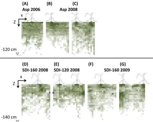
Root density was characterized in 2008 and 2011 at the end of the maize cycle. The data collected in both years were further enriched by data collected by former similar works performed at the Lavalette station, available from its database. In all cases, the simple method of Tardieu and Manichon, (1986) was applied (e.g., Mubarak et al., 2009a). According to this method, soil pits (about 2.0 m long, 1.0 m wide and 1.8 m deep) were excavated at the harvest of each experimental campaign, perpendicularly to the maize rows. The faces of the pits were vertical planes, subdivided in square cells (5*5 cm). Root density was assessed based on visual observation. A number ranging from 0 to 5 was assigned to each cell according to the visually observed density in a 1 cm layer of the exposed soil surface.

Figure 2 shows the observed RDD profiles for Asp (A, B and C) and SDI (D, E, F, and G) plots (only 4 SDI profiles are illustrated for the sake of visibility).

215 216 217 218 219 220 221 222 223 224 225 226 227 228 229 230 231 232 233 234 235 236 237 238 239 240 241

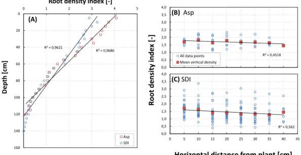
Figure 3A shows the mean vertical RDD (the means of each horizontal line) for both irrigation methods, whereas the mean horizontal RDD (the means of each vertical line) is shown in Figure 3B for Asp and Figure 3C for SDI plots.

Figure 2: Observed root density profiles of Asp (A, B, C) and SDI (D, E, F, G) maize plots. The driplines are presented by filled black circles. Root density was evaluated visually following the method of Tardieu et al. (1986). The observed profiles come from different experimental

campaigns as denoted for each profile.

Figure 3: The mean horizontal root density distribution (A) for both Asp and SDI maize plots, and the mean vertical root density of Asp (B) and SDI (C).

Since the root profiles are reconstructed from visual observations, the density indices are prone to the subjective evaluation made by the different observers and therefore these data are rather qualitative.

Roots were found to occupy the entire soil domain under maize rows and in the inter-row space, for both irrigation methods (Figure 2). Only a small decrease in root density was observed as the horizontal distance from the crop row increases (Figure 3B and C). Moreover, both Asp and SDI methods result in similar vertical RDD, with slightly higher density values for Asp in the upper 40 cm soil layer (Figure 3A). Furthermore, an interesting indication appears in Figure 2 for the SDI maize profiles: root density seems independent of the irrigation method, since no systematic increase in root density was observed in the vicinity of the drippers (represented by a blue circle), even for the same plot (Figure 2E).

The aforementioned observations do not plead in favor of the use of RDD profiles that are specific to a watering method. The results suggest that a 2D RDD profile where the root density decreases linearly, in both vertical and horizontal directions, adequately describes root systems (and consequently the potential RWU pattern) for both Asp and SDI systems. This observed RDD profile, denoted βObs, was used in the 10 242 243 244 245 246 247 248 249 250 251 252 253 254 255 256 257 258 259 260 261 262 263 264 265 266 267 268 269 270 22

numerical analysis with 5 additional hypothetical RDD profiles as will be further described in section 2.3.

2.2. Numerical analysis

2.2.1. Water flow simulation model

The Hydrus (2D/3D) model was used to simulate water flow in the soil by a numerical solution to the Richards equation (Richards, 1931) supplemented with a term S to account for root water uptake. To reduce the number of the spatial dimensions from three to two, it is assumed that water flow occurs only in a vertical plane perpendicular to the crop rows. This assumption stands for sprinkler irrigation as long as water application is uniform over the soil surface in the row direction. For SDI, it is assumed that water bulbs formed by the emitters overlap and merge forming a continuous cylindrical wetted zone along the dripline rendering thus water flow a 2D problem (Lafolie et al., 1989).

Considering the aforementioned assumptions and considering the soil to be isotropic, the equation describing the flow in a vertical plane is:

∂ θ/∂ t=∂

(

k (h , z )∂ h

∂ x

)

/

∂ x +∂

(

k (h , z ) ∂ h

∂ z

)

/

∂ z−∂ k (h , z )/∂ z−S

where x and z are respectively the horizontal and vertical (positive upwards) Cartesian coordinates [L]. The macroscopic RWU sink term S is given by:

S=T

γ (h ) β ( x , z ) φ

where Tp [L T-1] is the potential transpiration, γ(h) is the transpiration reduction function [-], β(x,z) is the potential RWU pattern which is identical to root density distribution RDD [L L-2], and finally ϕ is the compensatory uptake function of Jarvis (1989): φ=

{

where ω is the plant stress index (Ta/Tp) and ωc is a critical stress index threshold (see

Jarvis, 1989 and Simunek and Hopmans, 2009 for details).

In the present study, the piece-wise stress-response reduction function of Feddes et al. (1978) was used:

γ=

{

0 ; h≥ h

(

h

−

h)/(h

−

h

)

; h

>

h ≥ h

1; h

>

h ≥ h

(

h−h

)/(

h

−

h

)

; h

>

h≥ h

0 ; h

>

h

The values of h2 and h3 represent the thresholds between which water uptake is assumed maximum, while h1 and h4 represent respectively the thresholds of oxygen deficiency due to soil saturation and the minimum soil water content observed in the core of the root system (generally close to the wilting point). The values of h1, h2 and h4 were taken equal to -15, -30 and -15000 cm, respectively. Feddes et al. (1978) suggested that the value of h3 depend on the transpiration rate. h3 is therefore assumed to decrease as the transpiration rate decreases. Thus, h3 was taken equal to -325 and -600 cm for transpiration rates of 5 and 1 cm day-1_{, respectively. The} parameters values of the Feddes et al. (1978) function were fixed for all simulations.

Finally, the actual transpiration is calculated as the integral of S over the root zone (ΩR):

T

=

T

_∫

❑

γ ( h) β ( x , z ) φ d Ω

The different normalized root density distribution functions β(x,z) used in the present study will be detailed in subsection 2.3.

2.2.2. Soil domain characteristics

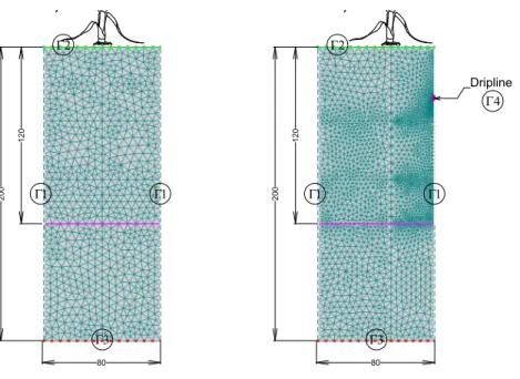
The width of the soil domain was set so that a zero horizontal flux Neuman-type boundary condition (BC) may be assumed across the lateral vertical boundary

12 295 296 297 298 299 300 301 302 303 304 305 306 307 308 309 310 311 312 313 314 315 316 317 26

elements (Figure 4). The soil domain was thus centered over a crop row, and the soil surface width was taken equal to the spacing between two maize rows (80 cm) in Asp and RF plots. The width of SDI plots was taken equal to the half of the distance between two drip lines, assuming that a zero horizontal flux occurs on both verticals under the dripline, and at mid-distance between two driplines.

Figure 4: The geometry and boundary conditions (BC's) imposed to the soil domains with dimensions given in cm. Γ1 is a zero horizontal flux BC, Γ2 is an atmospheric BC, Γ3 is a constant

water-content BC and Γ4 is a variable flux BC. The horizontal pink line at 120 cm represents the

maximum root depth at which drainage was calculated.

The depth of the soil domain was set so that a Dirichlet-type constant soil-water content BC may be considered at the lower soil boundary. The depth at which changes in the value of θ were negligible was approximately 190 cm for most treatments. Therefore, the maximum depth of the soil domain was set to 200 cm.

Finally, on the soil surface, an atmospheric variable fluxes BC was imposed. All atmospheric fluxes were assumed to be uniformly distributed over the soil surface. While daily rainfall fluxes where readily available from meteorological station records, the daily potential fluxes of crop transpiration Tp and soil evaporation Ep had to be calculated from the daily ETM, using an external crop model.

The Pilote model (Mailhol., 1997; Mailhol et al., 2011) was used to separate ETM into Tp and Ep, as a function of the LAI according to Ritchie (1972) and Novak (1981). This model has been shown to yield good predictions of soil-water reserves, LAI and biomass production of maize crop in the pedo-climatic context of the Lavalette station, for surface irrigated plots, subsurface irrigated plots (Mailhol et al., 2011), both for tillage and no tillage practices (Khaledian et al., 2009). Pilote is a one dimensional bucket-type model. This model assumes the soil domain to be homogeneous and isotropic over the entire root zone, and the crop water use to be optimum as long as the lumped soil-water reserve of the root zone is greater or equal to the readily 318 319 320 321 322 323 324 325 326 327 328 329 330 331 332 333 334 335 336 337 338 339 340 341 342 343 344 345

available water. Therefore, Pilote is root density-independent and the resulting Tp and Ep fluxes of each plot may be used in Hydrus (2D/3D) simulations regardless of the β profiles used.

Finally, the vertical soil profile of the Lavalette station shows 3 layers distinguished with specific hydrodynamic properties. Mubarak et al. (2009a) fitted soil hydrodynamic parameters to the van Genuchten-Mualem model (van Genuchten, 1980; Mualem, 1976), as described in Table 1.

Table 1: The hydrodynamic parameters of the van Genuchten-Mualem model (van Genuchten,

1980; Mualem, 1976) model fitted to the soil of Lavalette station. θr and θs denote respectively

the residual and saturated volumetric soil water contents, α and n are empirical shape parameters, Ks is the soil hydraulic conductivity at saturation and l is a pore connectivity

parameter.

2.3. Scenarios

To summarize:

The Hydrus (2D/3D) model was run for the simulation of water flow in the soil of 11 treatments cultivated with maize:

AspETM (11) and AspETM (12): sprinkler, fully-irrigated treatments in 2011 and 2012,

Asp70ETM (08), Asp50ETM (11) and Asp50ETM (12): sprinkler, deficit-irrigated treatments (30% deficit in 2008 and 50% deficit in both 2011 and 2012),

SDI (08), SDI (11) and SDI (12): SDI, deficit-irrigated treatments (30% deficit in all 3 years),

RF (08), RF (11) and RF (12): rainfed treatments in 2008, 2011 and 2012.

14 346 347 348 349 350 351 352 353 354 355 356 357 358 359 360 361 362 363 364 365 366 367 368 369 370 30

For each of the 11 treatments, water flow was simulated for 36 scenarios (6 β profiles and 6 ωc levels). The levels of ωc ranged from 0.5 (the maximum compensatory uptake level considered) to 1.0 (non-compensatory uptake). The 6 β profiles are illustrated in Figure 5:

1. The “observed” RDD profile (βObs): root density decreases linearly in both the vertical and horizontal directions, as discussed in section 2.1.2.

2. The “sprinkler-specific” profile (βAsp): root density decreases exponentially in both the vertical and horizontal directions. This profile was constructed using the Vrugt et al. (2001) function, implemented in the Hydrus (2D/3D) model. We hypothesize by using this profile that root activity is mainly concentrated in the shallow soil layers since irrigation is applied at the soil surface.

3. and 4. Two “SDI-specific” profiles, respectively βSDI-1 and βSDI-2: the maximum root density is located in the vicinity of the dripper (βSDI-1) or at the same depth of the dripper on the vertical of the plant row (βSDI-2). Those two profiles were selected to correspond to match the cases were root density was observed to increase near the drippers (Figure 2F, G). We hypothesize thus that uptake activity of the roots mainly takes place at deeper layers as a response to the subsurface allocation of irrigation water.

5. A constant root density profile (βCst): one may suggest that βCst represents an average profile that may be used in the case were an a-priori knowledge of the real root density is missing, as suggested by Kandelous et al. (2012).

6. Finally, a profile of increasing root density with depth (βInc) was added. βInc is horizontally constant but increases linearly with depth. Although βInc is in total contradiction with the observations of root systems of most biomes (Schenk and Jackson, 2002), one may hypothesize that such profile may reflect an increase uptake 371 372 373 374 375 376 377 378 379 380 381 382 383 384 385 386 387 388 389 390 391 392 393 394 395

activity of deep roots as soil surface dries out (e.g., Klepper, 1991). The addition of this profile aimed principally to maximize the contrast in the examined RDD profiles.

Figure 5: Root density profiles of fully-developed maize irrigated with SDI with driplines located on the right-side boundary at a depth of 40 cm. X* _{and Z}* _{are the horizontal and vertical}

coordinates at which the root density is maximum. Xmax and Zmax delimit the soil region

occupied by roots. Px and Pz are empirical shape parameters (specific to the function of Vrugt

et al. (2001).

The numerical scheme of the simulations for each of the 11 treatments is shown in Figure 5. Since Hydrus (2D/3D) does not simulate the increase of root depth with time, a series of simulations had to be put end-to-end for each treatment, where the Zmax was assumed to be constant within the period of each simulation. Zmax values were fixed to 30, 45, 75, 105 and 120 cm. The corresponding periods of the growth cycle were given by Pilote which simulates the increase of Zmax as a function of the cumulative degree-day temperatures. This temporal delimitation increased the number of the simulations to total 1980 (11 treatments * 6 β * 6 ωc * 5 end-to-end sequences). However, through all the simulated period, drainage was calculated at the depth of 120 cm, beyond which root density is assumed to become negligible.

Finally, for each of the simulations, the initial conditions were either predefined by observed θ profiles during the first growth period with Zmax equal to 30 cm, or read from the final time step of the previous simulation. On a personal computer (2.40 GHz processor, 32-bits, 4.00 GB RAM), the run of all simulations took approximately 24 hours.

Figure 6: Flowchart of the simulations conducted using Hydrus (2D/3D).

2.4. Statistical analysis of the results

For each treatment, observed and simulated θ profiles (θobs and θsim, respectively) were compared in order to determine the optimum simulation configuration (the choice of β profile and ωc levels). The statistics adopted for the comparison were the 16 396 397 398 399 400 401 402 403 404 405 406 407 408 409 410 411 412 413 414 415 416 417 418 419 420 421 422 423 34

correlation coefficient of Pearson (ρ) and the root-mean-square error (RMSE). In this context, the errors were only different from zero when θsim fell outside the associated confidence intervals (CI) of the measurements of θobs determined by the instrument and calibration curves.

Both ρ and RMSE are complementary measures. The Pearson’s ρ describes the linear relationship between two continuous random variables regardless of their values. Therefore, a high value of ρ means that a strong correlation between θobs and θsim exists, indicating thus that water distribution pattern is reasonably simulated (parallel θ profiles). However, this does not mean that both simulated and observed profiles are close, hence the need for an estimate of the error by means of RMSE. To determine whether the obtained RMSE values differed significantly following values of β and ωc statisticall tests have to be performed. In this respect, as it was found that errors {ε} = {|θobs - θsim - CI|} increased with depth, their statistical distribution was biased and did not adhere to normality. Therefore, the statistical analyses of RMSE results was performed using nonparametric tests. Firstly, the Kruskal-Wallis (K-W) test was used to determine whether β had a significant effect on ε for each ωc value. Secondly, when the results of the K-W test indicated a significant effect of β, the post-hoc test of Dwass-Steel-Critchlow-Fligner pair-wise test was performed to determine the significance of differences among the results.

3. Results

3.1. Transpiration

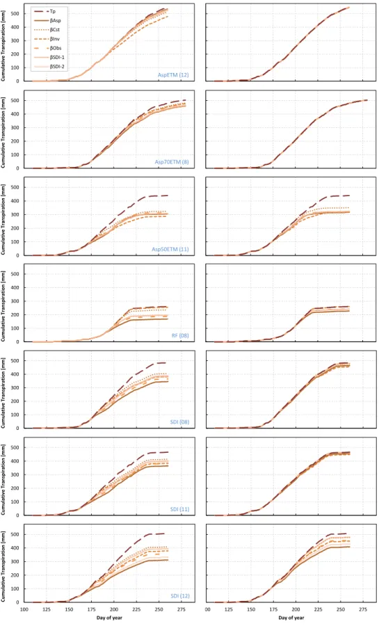
The results of the simulated transpiration fluxes are illustrated in Figure 7 for selected treatments of each watering method. In order to increase the readability of the results, the cumulative transpiration curves (Ta cum) are illustrated only for the non compensatory (ωc = 1.0) and the maximum compensatory (ωc = 0.5) RWU levels. The corresponding differences in Ta cum [mm] between those two latter cases are summarized in Table 2. 424 425 426 427 428 429 430 431 432 433 434 435 436 437 438 439 440 441 442 443 444 445 446 447 448 449 450

Figure 7: The cumulative transpiration curves Ta cum simulated with non compensatory (left

column) and the maximum compensatory (right column) RWU levels.

Table 2: The differences between the maximum and the minimum simulated cumulative transpiration Ta cum for each treatment, using all β profiles (columns 2 to 5) and only those of

the “realistic” group (columns 6 to 9).

Surface-watering simulations

In sprinkler treatments, using contrasted β profiles resulted in differences in Ta cum within the range of 22 to 63 mm, representing respectively 4.5% and 14.0% (1-min/max %) as shown in Table 2 (columns 2 and 3). These differences were higher for fully-irrigated treatments than for those deficit-irrigated. However, for all irrigation levels, the simulation with the maximum compensatory RWU level considerably reduced the effect of β, to produce, in the cases of AspETM (12) and Asp70ETM (08), almost identical total Ta cum values (Table 2, columns 4 and 5).

Similar results were obtained for rainfed treatments, even though the simulated Ta cum showed a higher sensitivity to β. Contrasted β resulted in higher differences in Ta cum, ranging from 28 to 87 mm which represent respectively 15.4% and 34.1% (Table 2, columns 2 and 3). These differences were considerably reduced to about 13% for all treatments when the compensatory RWU was activated (Table 2, columns 4 and 5).

The aforementioned differences in Ta cum come principally from βCst and βInv. When the latter are not considered, the simulated differences in Ta cum become considerably lower (Table 2, columns 6 to 9). The profiles βAsp, βObs, βSDI-1 and βSDI-2 resulted in very similar transpiration rates even when no compensatory RWU was considered. The corresponding differences between Ta cum maxima and minima were then between 2.0 and 7.5%, but in absolute water depth terms were all smaller than 16 mm.

18 451 452 453 454 455 456 457 458 459 460 461 462 463 464 465 466 467 468 469 470 471 472 473 474 475 476 477 38

The results of surface-watering simulations are not very sensitive to the spatial distribution of root density RDD, provided that the latter decreases linearly or exponentially with depth as observed for most realistic plant biomes by Schenk and Jackson (2002). In this case, considering compensatory RWU yielded only a limited effect on the simulated Ta cum, where the differences between Ta cum minima and maxima were all reduced by less than 13 mm (Table 2, columns 8 and 9), except for the case of RF (11) where those differences were increased using the compensatory uptake function.

SDI simulations

Root density distribution played a greater role in the determination of transpiration rates in SDI treatments.

Considering for instance only β profiles of the “realistic” group (βAsp, βObs, βSDI-1, βSDI-2): βAsp and βSDI-1 systematically resulted in the lowest and the highest transpiration rates, respectively (SDI results in Figure 7, left column). For non compensatory water uptake, the differences between Ta cum maxima and minima ranged from 37 mm (9.2%) for the case of SDI (11) to as much as 83 mm (21.1%) for that of SDI (12), (Table 2, columns 2 and 3). This greater difference obtained in 2012 was due to the higher plant-dripline distance (65 cm) compared to 2008 and 2011 (40 and 30 cm, respectively). Consequently, β profiles with maximum root densities located beneath the plant row resulted in considerably lower water uptake compared to βSDI-1.

However, activating the compensatory RWU function considerably reduced the differences between Ta cum maxima and minima, but this decrease strongly depended on the plant-dripline distance. While those differences were reduced by 27 mm in both 2008 and 2011 (62% and 72%, respectively), the compensatory uptake resulted in a limited reduction of only 12 mm (15%) in Ta cum (max-min) in the case of 2012 (Table 2, column 6 compared to column 8). Furthermore, for the case of 2012, more enhanced 478 479 480 481 482 483 484 485 486 487 488 489 490 491 492 493 494 495 496 497 498 499 500 501 502 503 504

transpiration was simulated with βObs profile than with that of βSDI-2 since the latter had less root density in the vicinity of the dripper compared to βAsp.

3.2. Drainage

Similar to the previous section, the simulated drainage outfluxes below the root zone (Z = 120 cm) are illustrated only for a selected number of treatments (Figure 8). The differences in the cumulative drainage outfluxes (Draincum) are summarized in Table 3.

Figure 8: Cumulative drainage/capillary rise outfluxes simulated with non compensatory (left column) and the maximum compensatory (right column) RWU levels. Vertical bars represent

rainfall and irrigation events.

Table 3: The differences between the maximum and the minimum simulated cumulative drainage Draincum outfluxes for each treatments, using all β profiles (columns 2 and 3) and only

those of the “realistic” group (columns 4 and 5).

Globally, the cumulative drainage outfluxes or capillary rise influxes followed the vertical distribution of root density, i.e. root profiles with higher root densities in lower soil layers resulted in systematically lower drainage rates or higher capillary rise (Figure 8). The simulations using βInv resulted in systematically the highest capillary rise rates, followed by the simulations issued from the βCst, then those of βSDI-1 and βSDI-2 (both being quasi-identical for all sprinkler and rainfed simulations), then βObs and βAsp last.

Surface-watering simulations

Two groups of Draincum curves are clearly distinguished in Figure 8: those resulting from the “realistic” (βAsp, βObs, βSDI-1 and βSDI-2) and those from the “atypical” (βCst and βInv) profiles. 20 505 506 507 508 509 510 511 512 513 514 515 516 517 518 519 520 521 522 523 524 525 526 527 528 529 530 42

The compensatory uptake had a limited effect on Draincum (Table 3): it reduced Draincum by less than 6 mm in all simulations of the surface-watering treatments, but failed to reduce differences of Draincum (max-min). The latter were merely the same with and without compensatory uptake. These results indicate that, in the case of surface-watering conditions, the effect of the compensatory RWU function on the reduction of the sensitivity of the simulated drainage is negligible.

SDI simulations

The sensitivity of drainage prediction to the spatial distribution of root density was considerably higher under SDI conditions, as may be seen from Figure 8.

In addition to the vertical distribution of root density, the simulated Draincum depended on the position of the plant row relative to the dripline. For instance, for similar total irrigation depths in 2008, 2011 and 2012, the lowest drainage rates were obtained with βSDI-1and βSDI-2, in 2008 and 2011, but not in 2012 when βSDI-2 resulted in considerably higher drainage outfluxes due to higher plant-dripline distance.

Compensatory RWU efficiently reduced both the absolute value of drainage outfluxes and the relative differences resulting from the contrasted β profiles (Table 3 columns 3 and 5 compared to columns 2 and 4, respectively). The plant-dripline distance also conditioned the efficiency of the compensatory uptake function. The reduction rates were greater with smaller plant-dripline distance : the simulated Draincum in the case of SDI (12), using βAsp, was reduced by 35 mm for a ωc of 0.5, while only a reduction of 5.3 mm was obtained in the case of SDI (11), for the same conditions (Table 3).

The compensatory uptake has thus a non negligible effect on the reduction of the sensitivity of Hydrus (2D/3D) model to the β function, when it comes to drainage simulation in SDI treatments. However, strong discrepancies in simulated drainage outfluxes were still mainly explained by the β function. One may thus suggest that, in the context of a macroscopic, empirical, RWU model as such implemented in Hydrus 531 532 533 534 535 536 537 538 539 540 541 542 543 544 545 546 547 548 549 550 551 552 553 554 555 556 557 558

(2D/3D), reasonable predictions of drainage outfluxes may require the use of β profiles that are watering method-specific (water-tracking). This hypothesis is verified by the comparison of the observed θ profiles to those simulated, describing the RWU patterns.

3.3. RWU patterns

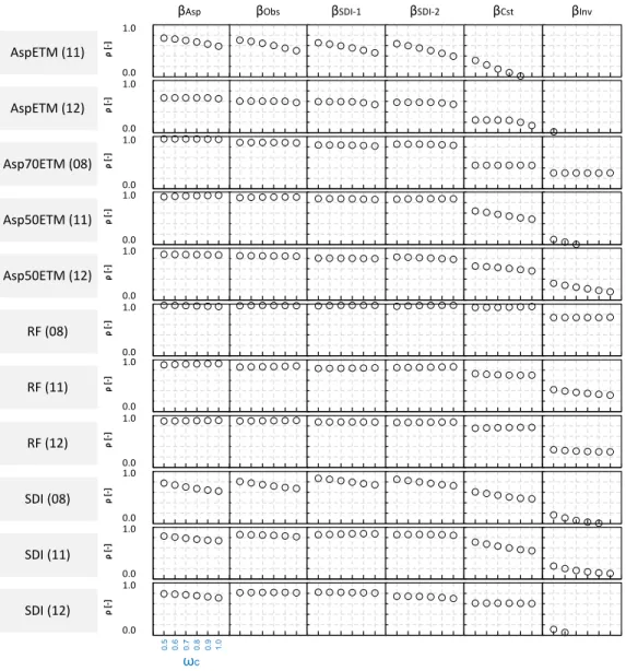
The values of Pearson correlation coefficient (ρ) between θobs and θsim for all scenarios are shown in Figure 9.

Figure 9: Correlation coefficient of Pearson (ρ) between θobs and θsim profiles for all scenarios.

Only the positive ρ values are shown.

Three main points are drawn from the results of the correlation test:

1. The compensatory RWU process does not have a systematic effect on the improvement of the predictions of RWU patterns: only the cases of AspETM (11) and SDI (08) showed an increased value of ρ following an increase of ωc, while for the rest of the simulations the compensatory RWU had a very limited effect on ρ.

2. For the βCst and βInv profiles, the poor values of ρ were improved with compensatory RWU, but never reached those of the other realistic profiles (βAsp, βObs, βSDI-1 and βSDI-2). This shows the limits of the efficiency of the compensatory RWU when used with a poor representation of root density.

3. Water-tracking β profiles result in the best correlations, with and without compensatory uptake: highest ρ values were obtained with βAsp and βSDI-1 respectively in surface-watering and SDI simulations.

The effects of ωc on ρ for each β are further examined via the RMSE values, summarized in Table 4 for the simulations of the non compensatory (a) and the compensatory (b) water uptake level of 0.5.

22 559 560 561 562 563 564 565 566 567 568 569 570 571 572 573 574 575 576 577 578 579 580 581 582 583 46

Table 4: Root-mean-squared errors (RMSE) [-] between θsim and θobs profiles for non

compensatory (a) and compensatory uptake (b) simulations. RMSE values followed by the same letters indicate no statistically significant differences (α = 0.5).

The results of the ρ statistic are confirmed by RMSE values: poor predictions of θ using βCst and βInv but better predictions using the β profiles of the “realistic” group. Moreover, all “realistic” profiles yielded simulations with similar RMSE values, while those of βCst and βInv resulted in significantly (α = 0.5) higher RMSE in most simulations. The lowest errors were obtained with βAsp for most surface-watering treatments, while the lowest errors in SDI treatments were obtained with the βSDI-1 profile.

While the differences in RMSE among simulations were reduced with compensatory RWU, their absolute values were unexpectedly increased for most simulations (Table 4b compared to Table 4a). To explain this increase, it will be necessary to graphically compare θsim to θobs profiles for both compensatory and non compensatory RWU simulations. This comparison is only performed for selected cases. The reader may refer to the supplementary materials to get access to the integrity of simulation results.

Surface-watering simulations

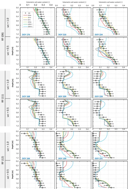
Figure 10: Comparison between θsim and θobs for all rainfed treatments, for non and maximum

compensatory RWU level. The horizontal bars represent measurement errors corresponding to the neutron probe calibration equation.

Reasonable agreements between θsim and θobs were obtained without compensatory RWU in rainfed treatments (Figure 10, rows 1, 3 and 5). Using the “realistic” β profiles resulted in predictions of θ within the observation confidence 584 585 586 587 588 589 590 591 592 593 594 595 596 597 598 599 600 601 602 603 604 605 606 607 608 609 610

intervals in RF (08) and RF (11), but slightly overestimated θ in deep soil layers in RF (12). In contrast, using βCst and βInv resulted in significantly higher and lower θ values in upper and lower soil layers, respectively.

The simulation with compensatory RWU slightly improved the predictions of θ in RF (11) and RF (12), by an enhanced water uptake in deeper soil layers (Z ≥ 40 cm), (Figure 10, rows 4 and 6). However, it led to an insignificant reduction of the predicted θ values (the θ profile remained within the confidence interval of measurements) when the βAsp was used in the case of RF (08), (Figure 10, row 2). This implies that the resulting increase of 59 mm (35%) in Ta cum obtained with the compensatory uptake using βAsp in 2008 is insignificant, and may thus be associated to the sensitivity of Hydrus (2D/3D) to the spatial distribution of root density. Moreover, in RF (08) the compensatory RWU led to significantly underestimate θ in deep soil layer, when βAsp was not used. This indicates that root density distribution is the factor that mostly determine water uptake pattern, with and without the compensatory uptake function. Furthermore, these results suggest that a compensatory mechanism did not take place in the rainfed treatment of 2008, and that for rainfed treatments of 2011 and 2012, improvements in water-content predictions may have simply been achieved by modifying the parameters of the Feddes stress function (more tolerance to drought).

Similar results were obtained concerning the deficit-irrigated sprinkler treatments (data not shown), but with the compensatory function slightly improving predictions of θ in upper soil layers by an enhanced water uptake following watering. Nonetheless, this enhanced uptake activity failed to mimic water uptake pattern in the more dynamic watering conditions of the fully irrigated sprinkler treatments (AspETM 11 and AspETM 12), as shown in Figure 11.

Figure 11: Comparison between θsim and θobs for the fully-irrigated sprinkler treatments, for non

and maximum compensatory RWU level. The horizontal bars represent measurement errors corresponding to the neutron probe calibration equation.

24 611 612 613 614 615 616 617 618 619 620 621 622 623 624 625 626 627 628 629 630 631 632 633 634 635 636 637 638 50

Strong discrepancies were obtained in the fully-irrigated sprinkler treatments between all θsim and θobs (Figure 11). From mid-season (DOY 170-180), all simulated profiles showed a systematic overestimation of RWU in soil layers between 40 and 90 cm depths, and underestimated RWU in shallow soil layers. Given the reasonable estimations of plant water requirements by Pilote (Appendix A1) and the fact that irrigation and rainfall amounts were gauged directly in the vicinity of the instrumented plots; it is unlikely that those discrepancies come from errors in the estimations in either of Ta or water influxes rates.

When these discrepancies are further prone to increase with compensatory RWU (see values of RMSE in Table 4b compared to Table 4a), one may then suggest that such systematic discrepancies may only be suppressed by changing the root profile, by increasing root density in the upper layers. This hypothesis was verified by performing the simulations of both fully-irrigated treatments using a new root profile: βETM. The root density of βETM is horizontally constant, but the density index (adimensional) decreases linearly from 1.0 to 0.1 between depths of 0.0 and 30.0 cm, then decreases linearly to reach 0.0 at a depth of 120.0 cm. These simulations were only performed for two compensation levels : ωc = 1.0 and ωc = 0.5. The resulting θ profiles are shown in Figure 12 only for simulations using βAsp and βETM.

Figure 12: Comparison between θsim and θobs for the fully-irrigated treatments. The simulations

were conducted using βAsp and βETM profiles, for non and maximum compensatory RWU level.

The horizontal bars represent measurement errors corresponding to the neutron probe calibration equation.

Substantial improvements were obtained when βETM profile was used (Figure 12). Better agreements between θsim and θobs were achieved for both ωc values in AspETM (12), but only for ωc = 1.0 (non compensatory uptake) in the case of AspETM (11). In the latter case, Ta cum was equal to 459 mm compared to 502 mm with compensatory 639 640 641 642 643 644 645 646 647 648 649 650 651 652 653 654 655 656 657 658 659 660 661 662 663 664 665

uptake, i.e. an overestimation of 43 mm (9.4%) resulted from considering compensatory RWU.

This result confirms the former observations, in rainfed and deficit-irrigated sprinkler treatments, on the role of the β function being the main factor to determine water extraction pattern. In addition, this result points out to the possibility of an overestimation of transpiration when the compensatory uptake is considered.

SDI simulations

Due to the inherent high spatial heterogeneity of soil water-content in SDI treatments, the comparison between θsim and θobs was performed on two verticals: the first on the crop row and the second in the immediate vicinity of the dripline (Figure 13) where measures of θ were only available in 2011 and 2012.

Figure 13: Comparison between θsim and θobs under plant row and dripline for SDI (11) and SDI

(12), for non and maximum compensatory RWU levels. The horizontal bars represent measurement errors corresponding to the neutron probe calibration equation.

Both β and the compensatory RWU function were determinant factors to achieve reasonable predictions of θ profiles. Best agreements between θobs and θsim were obtained under both crop row and dripline when βSDI-1 was used in combination with the maximum compensatory RWU level (Figures 13). An interesting observation in Figure 13 is that of SDI (12) on DOY 214 and 242, where βSDI-1 allowed to obtain remarkably close predictions of θ profile, despite the relatively long plant-dripline distance of 65 cm. However, in some cases the compensatory RWU resulted in significant underestimation of θsim in upper soil layers under the crop row during earlier growth stages .

The results indicate that RWU is strongly underestimated if the compensatory RWU is not considered. Moreover, even for the maximum compensatory level, RWU is underestimated if βSDI-1 is not used (e.g., final observation dates in Figure 13). For 26 666 667 668 669 670 671 672 673 674 675 676 677 678 679 680 681 682 683 684 685 686 687 688 689 690 691 692 693 54

instance, for SDI (08), SDI (11) and SDI (12), using βAsp instead of βSDI-1 underestimate plant transpiration by respectively 43, 37 and 83 mm with non compensatory RWU, or respectively by 16, 10 and 71 mm when a compensatory RWU is considered.

Due to the more dynamic pattern of water allocation in SDI treatments (by both rainfall and dripline), maximum root activity is expected to alternate between the soil regions at surface and near the dripper, an activity that a static root density profile fail to mimic. Using the compensatory RWU allowed to overcome this shortcoming of static β profiles. However, reasonable predictions of RWU activity was only achieved combining a high compensatory RWU level with a water-tracking root density profile. The latter was then found to be the determinant factor for reasonable RWU simulation in SDI treatments.

4. Discussion

4.1. The efficiency of the compensatory root water uptake function ϕ

Let us recall the definition of the compensatory RWU process as proposed in the pioneer work of Jarvis (1989): the ability of plants to compensate stress-induced reduction of water uptake in one part of the root zone by an enhanced uptake from other parts where soil water is more readily available. On the one hand, we showed that using the compensatory RWU function efficiently increased the values of ρ between observed and simulated θ profiles, indicating thus better “overall” mimicking of RWU pattern. However, on the other hand, the compensatory RWU led to larger prediction errors {|θobs - θsim - CI|}, which means that these errors came from enhanced water uptake in the “wrong” soil regions:

1. In surface-watering simulations, the enhanced RWU by the compensatory process took place mainly in deep soil layers. When rainfed treatments are considered, RWU was not observed to be enhanced in deep soil layers in all treatments. When fully-irrigated sprinkler treatments are considered, enhanced 694 695 696 697 698 699 700 701 702 703 704 705 706 707 708 709 710 711 712 713 714 715 716 717 718 719

RWU was observed in the uppermost soil layers due to the surface irrigation regime.

2. In subsurface drip irrigation simulations, the enhanced RWU by the compensatory process led to obtain remarkably good agreements between θobs and θsim under the dripline when root density was adequately described. However, since the compensatory rate is proportional to the Ta/Tp ratio (Eq. 5) rather than soil-water content spatial distribution, the enhanced RWU was not limited to soil regions around the drip water source, but occurred in the entire root zone. Consequently, simulated enhanced RWU also occurred beneath the plant row contrarily to observations.

Points 1 and 2 indicate that the compensatory RWU process may hardly be seen as a response to the total plant stress status ratio Ta/Tp. Our results suggest that the compensatory RWU pattern depends on the distribution of water through the soil domain, rather than plant water deficit.

The results of this study are in agreement with a recent study on RWU pattern conducted by Javaux et al. (2013). Using a physically-based macroscopic RWU model developed by Couvreur et al. (2012), Javaux et al. (2013) found that the compensatory RWU rate is independent from the ratio (ω/ωc). Both studies of Couvreur et al. (2012) and Javaux et al. (2013) further proposed a decoupling of the water stress function γ(h) from that of the compensatory RWU, since the latter occurred even at very low water potential levels. The compensatory RWU is thus perceived as the redistribution of RWU due to a nonuniform water head distribution at the soil–root interface.

A number of examples of empirical compensatory RWU functions which are independent from the Ta/Tp ratio exists in literature (e.g., Bouten et al., 1992; Lai and

Katul., 2000; Li et al., 2001). However, such models are also shown to be highly dependent on root density (see Heinen, 2014 for the case of the function of Bouten et al., 1992), and still couple the water stress and compensatory processes. An

28 720 721 722 723 724 725 726 727 728 729 730 731 732 733 734 735 736 737 738 739 740 741 742 743 744 745 746 58

interesting approach to RWU simulation would be to extrapolate the propositions of Couvreur et al. (2012) and Javaux et al. (2013) for the modeling of empirical macroscopic RWU models. Such extrapolation may replace Equation 4 for the calculation of RWU by another one of the form:

S=T

β ( x , z )

[

γ (h )+φ(h)

]

The quantity Tp β(x,z) γ(h) in Equation 8 represents RWU in standard conditions (uniform soil water potential over the entire root zone), while the quantity Tp β(x,z) ϕ (h) represents the instantaneous adjustment of RWU distribution to cope with the variations of soil water potential in the root zone. For example, the distribution of the values of ϕ(h) may be deduced from moment analysis of the spatial distribution of soil water potential. Furthermore, analogously to the formula proposed by Couvreur et al. (2012), the sign of ϕ(h) may be positive (enhanced uptake) or negative (hydraulic lift). However, more research is needed to propose a formula for the ϕ(h) that respects the condition (Ta ≤ Tp). Such work is beyond the scope of the present study.

4.2. The role of root density distribution

Warrick and Or (2007) stated that “often no distinction is made between root length density and root activity or uptake”. Maintaining the current formula of the RWU function (Eq. 2 and 4) implies that all roots are considered active. Therefore, β must reasonably reflect the RWU activity. Both by experimental (e.g. Homaee et al., 2002; Hodge, 2004) and numerical analysis (Bruckler et al., 2004; Faria et al., 2010), RWU activity was widely reported to employ only a limited percentage of the entire root system.

It was shown in section 3 that β has a determinant role in the prediction of RWU pattern, under all water stress conditions. It was shown in Figure 9 and Table 4 that better predictions of θ were obtained when root profiles specific to the watering method were used: βETM in fully-irrigated sprinkler treatments, βAsp in deficit-irrigated sprinkler treatments and βSDI-1 in SDI treatments.

747 748 749 750 751 752 753 754 755 756 757 758 759 760 761 762 763 764 765 766 767 768 769 770 771 772 773

By numerical analysis with a physically-based RWU model, Bruckler et al. (2004) found that surface watering events resulted in roots having high instantaneous water uptake rates. Consequently, only a limited number of roots assured the full water requirements by plants. The results of the present study are in agreements with the findings of Bruckler et al. (2004). It was shown in section 3 that a correct prediction of RWU pattern, in fully-irrigated sprinkler treatments, was obtained if and only if a specific β profile (βETM), having the maximum root density in the uppermost soil layers, was used. In SDI treatments, reasonable prediction of RWU pattern required both a high compensatory RWU level and a root profile with maximum density near the dripper.

These results plead in favor of the use of water-tracking RWU, particularly in the case of locally-watered soil domains where a reasonable prediction of RWU pattern requires both a pertinent description of the spatial distribution of root density and a high compensatory uptake level. In that sense, when Equation 4 is used to describe RWU, the β function should not only reflect the potential RWU pattern according to root density, but also according to the expected soil-water availability (i.e., watering influx distribution). This recalls the early definitions of β as “root effectiveness function” as stated by Whisler et al. (1968). Thus, by using a watering method-specific β, the aim is to increase the probability of an enhanced water uptake in predefined wetter soil regions.

Another issue related to root density distribution is its relation to the simulated water outfluxes from the soil domain. Ta is the integral of the spatially-distributed RWU (Eq. 7). Therefore, it is expected that different root density profiles may lead to similar transpiration rates. By comparing 4 different RWU models, going from empirical macroscopic to physically-based microscopic, de Willigen et al. (2012) found that differences in total transpiration were small compared to those of the simulated soil-water dynamics. The authors explained their results by the feedback process between the RWU and water flow models. This shows that the determination of the “best” RDD

30 774 775 776 777 778 779 780 781 782 783 784 785 786 787 788 789 790 791 792 793 794 795 796 797 798 799 800 801 62

function or compensatory RWU level based solely on comparisons to measured Ta is a condition necessary but not sufficient. This confirms the pertinence of the choice to base our analysis on the comparison between θsim and θobs, which not only allows an insight to RWU pattern, but also assures mass balance conservation (Ta cum).

Finally, our results showed that using a uniform β profile, when relevant information on root system is missing, may lead to poor estimates of plant transpiration and drainage fluxes as well as RWU pattern, under both surface and subsurface waterings. Such consideration may thus bias the evaluation of optimum SDI design when an inappropriate β profile is used, as performed by Kandelous et al. (2012).

4.3. The performance of the empirical macroscopic RWU approach

The empirical macroscopic RWU models are often subject to critical comments ranging from too little biophysical basis (Skaggs et al., 2006; Javaux et al., 2008; Schneider et al., 2010; Javaux et al., 2013) to too many parameters requiring calibration (Feddes et al., 2001; Homaee et al., 2002; Couvreur et al., 2012; de Willigen et al., 2012), and questionable performance in heterogeneous soils (Kuhlmann et al., 2012).

However, the results obtained in this study show a rather robust performance of this RWU approach in stratified soil profiles, under contrasted watering methods, watering dynamics and water stress status, provided that adequate descriptions of the root density distribution and compensatory levels are used. These were nonetheless the results of rather simple cases of a mono-crop cultivated soil domain, and are thus subject to vary for more complex systems, where more sophisticated physically-based models may be more efficient.

5. Conclusions

Using an empirical macroscopic root water uptake model integrated in a physically-based soil water flow model, a numerical analysis was performed to 802 803 804 805 806 807 808 809 810 811 812 813 814 815 816 817 818 819 820 821 822 823 824 825 826 827 828

examine the sensitivity of simulated actual transpiration (Ta), drainage (Draina) and root water uptake (RWU) patterns to both root density distribution (RDD) and compensatory RWU functions. The numerical analysis was based on simulations of water transfer in a vertical 2D soil domain cultivated with maize, irrigated by surface (sprinkler) or subsurface (SDI) systems, or rainfed. The simulations were compared to experimental data to estimate the errors in drainage rates due to uncertainties in the RDD, to study the effect of the compensatory RWU function on the sensitivity to RDD, and to verify whether the use of a water-tracking root density profile replaces the need for compensatory RWU functions. The principal findings of this study may be summarized in the following points:

1. The simulation of Ta, showed to be of low sensitivity to RDD in sprinkler-irrigated (Asp) and rainfed (RF) treatments, provided that root density decreases linearly or exponentially with depth. In contrast, RDD played a greater role in the determination of Ta in the case of subsurface drip-irrigated (SDI) treatments.

2. The simulation of Draina was found to vary considerably in all cases with the RDD.

3. The compensatory RWU function further reduced the sensitivity of the simulated Ta to RDD in surface-watering treatments and, to a lesser extent, in SDI treatments. The efficiency of the compensatory RWU function in SDI simulations depended on the plant-dripline distance.

4. The compensatory RWU function had low or no effect on the reduction of the sensitivity of the simulated Draina to RDD in surface-watering treatments. In contrast, compensatory RWU function played a considerable role in the reduction of differences resulting from different RDD profiles in SDI simulations. However, reasonable predictions of the RWU pattern were only achieved when a RDD profile specific to SDI was used with a high compensatory RWU level.

32 829 830 831 832 833 834 835 836 837 838 839 840 841 842 843 844 845 846 847 848 849 850 851 852 853 854 66

5. Using an empirical macroscopic RWU function, it was shown that the main condition for reasonable estimation of Ta, Draina and RWU pattern was to use water-tracking RWU.

6. Finally, the results suggest that the use of the compensatory RWU function of Jarvis (1989) is recommended for simulations with local water influx simulations (SDI), but questionable performance is expected in simulations were water influx is uniform over the soil domain surface (sprinkler).

Acknowledgments

The University of Aleppo, Syria, is greatly acknowledged for the PhD scholarship granted to Rami ALBASHA. The authors gratefully acknowledge Mr. Christian LEDUC, Mr. François AFFHOLDER and Mme. Séverine TOMAS for critically reading the manuscript. The authors also thank Mr.Jean-Marie LOPEZ, Mr. Patrick ROSIQUE and Mr. Augutin LUXIN for their assistance in data collection.

855 856 857 858 859 860 861 862 863 864 865 866