HAL Id: hal-00559950
https://hal.archives-ouvertes.fr/hal-00559950
Submitted on 26 Jan 2011
HAL is a multi-disciplinary open access
archive for the deposit and dissemination of
sci-entific research documents, whether they are
pub-lished or not. The documents may come from
teaching and research institutions in France or
abroad, or from public or private research centers.
L’archive ouverte pluridisciplinaire HAL, est
destinée au dépôt et à la diffusion de documents
scientifiques de niveau recherche, publiés ou non,
émanant des établissements d’enseignement et de
recherche français ou étrangers, des laboratoires
publics ou privés.
Virtual Roots of a Real Polynomial and Fractional
Derivatives
Daniel Bembe, André Galligo
To cite this version:
Daniel Bembe, André Galligo. Virtual Roots of a Real Polynomial and Fractional Derivatives.
Inter-national Symposium on Symbolic and Algebraic Computation (ISSAC), Jun 2011, San Jose, United
States. pp.27-34, �10.1145/1993886.1993897�. �hal-00559950�
Virtual Roots of a Real Polynomial and Fractional
Derivatives
Daniel Bemb ´e
Mathematisches Institut der Universit ¨at M ¨unchen Theresienstr. 39, D-80333 M ¨unchen, Germany
bembe@math.lmu.de
Andr ´e Galligo
∗Universite de Nice-Sophia Antipolis, Mathematiques
Parc Valrose 06108 Nice cedex 02, France
galligo@unice.fr
ABSTRACT
After the works of Gonzales-Vega, Lombardi, Mah´e,[11] and Coste, Lajous, Lombardi, Roy [6], we consider the virtual roots of a univariate polynomial f with real coefficients. Using fractional derivatives, we associate to f a bivariate polynomial Pf(x, t) depending on the choice of an origin a,
then two type of plan curves we call the FDcurve and stem of f . We show, in the generic case, how to locate the virtual roots of f on the Budan table and on each of these curves. The paper is illustrated with examples and pictures com-puted with the computer algebra system Maple. .
Key words: virtual roots; real univariate polynomial; Budan table; fractional derivatives; FDcurve; stem.
1. INTRODUCTION
In [13], Rahman and Schmeisser note that rules of signs for calculating the roots of a polynomial are older than calcu-lus. Nowadays subdivision methods, heirs of these rules, are widely applied for calculating good approximations of so-lutions of polynomial equations or intersections of surfaces in Computer Aided Geometric Design. The geometric dic-tionary in complex algebraic geometry between invariants readable on equations and features of varieties is ultimately based on the fact that a polynomial of degree n admits n roots. This is not the case for real roots, and make real algebraic geometry more complicated. A natural strategy for studying properties of real algebraic varieties is to con-sider simultaneously roots of iterated derivatives of the in-put. An important progress was achieved by Gonzales-Vega, Lombardi, Mah´e when generalizing the real roots, they in-troduced in [11] the notion of virtual roots of a polynomial. The n virtual roots of a degree n polynomial provide a good substitute to the n complex roots.
Tables containing the signs of all the derivatives of a poly-nomial f are called in this paper Budan tables. They were
∗and INRIA Mediterrann´ee, Galaad project team.
used by various mathematicians including R. Thom for sep-arating and labeling the different real roots of a polynomial, see [4]. Relying on Rolle theorem, we analyze the different admissible configurations of successive rows in such a table. Restricting to the generic case where all roots of all deriva-tives are two by two distinct, we identify the table with an infinite rectangle separated into positive and negative blocs. We study the topology of the positive (resp. negative) blocs components, and characterize the virtuals roots using con-nected blocs components.
We also view these connected bloc components inside the Budan table as plane surfaces delimited by discretized curves. To furtherexplore this analogy, we consider derivatives with non-integers orders called fractional derivatives. We point out that fractional derivatives of a polynomial admit a bi-variate polynomial factor. This bibi-variate factor is used to construct two kinds of real planes curves attached to f : FD-curves and stem. The roots of all derivatives of f lie on each curve. These curve naturally realize a partition of the plane, hence can be used to geometrically determine the sign of a derivative at any point. We discuss and illustrate with examples, the possibility of using these curves to ease the location of the virtual roots in a Budan table.
The paper is organized as follows. Section 2 presents the virtual roots and give a quick proof of their characterization by jumps in the sign variations, followed by the definition of virtual multiplicity. Then admissible configurations for a table to be a Budan table are identified. Section 3 ex-aminates what happens in the generic case and establishes our main connexity result. Section 4 is devoted to fractional derivatives and its applications to our setting, FDcurves are introduced and illustrated. Section 5 describe intersections of FDcurves (resp. stems) with a Budan table and their use for the location of virtual roots.
2. VIRTUAL ROOTS
In this section let R be the field of real numbers (more generally a real closed field). In [11] the virtual roots of a monic degree-n polynomial f ∈ R[X] were introduced. They provide n root functions ρn,k(1 ≤ k ≤ n) on the space
of all monic monic degree-n polynomials. In particular they have the following properties:
1. For every k the ρn,k : Rn → R are continuous
func-tions of the n coefficients (a0, . . . , an−1) ∈ Rn of the
monic polynomial f (X) = Xn+ a
2. if f (a) = 0 then a = ρn,kfor at least one k,
3. for every k we have ρn,k ≤ ρn−1,k ≤ ρn,k+1, where
ρn−1,k denotes the k-th virtual root of f0.
From an approximate computational point of view, the ad-ventage is that the coefficients need not been known with infinite precision in order to compute the virtual roots with finite precision.
We summarize some of the results of [11] and [2]. [6] shows that the Budan-Fourier count always gives the number of virtual roots (with multiplicities) on an interval. The au-thors of [6] present some of our results in the more gen-eral context of f -derivatives. At the end of this section we present the Budan table and some claim about the virtual multiplicity.
2.1 Definition
Definition 2.1 (Virtual roots). Let f ∈ R[X] monic of degree n and f(i)denote its i-th derivative. For 0 ≤ j ≤ n
the j virtual roots of f(n−j), ρ
j,1 ≤ · · · ≤ ρj,j, are defined
inductively:
1. Let ρj,0= −∞ and ρj,j+1= ∞ for 0 ≤ j ≤ n.
2. For fixed 1 ≤ j ≤ n let be the ρj−1,k defined such that
for 1 ≤ k ≤ j
f(n−j+1)(x)f(n−j+1)(y) ≥ 0
for all x, y ∈ Rj−1,k = [ρj−1,k−1, ρj−1,k] (resp. the
half-open interval if k ∈ {1, j}).
3. Then for every 1 ≤ k ≤ j the ρj,k∈ Rj−1,k is defined
by the inequality |f(n−j)(ρ
j,k)| ≤ |f(n−j)(x)|
for all x ∈ Rj−1,k. This is well-defined since f(n−j)is
strictly monotone on Rj−1,k.
We must distinguish three cases: (a) ρj−1,k−1= ρj−1,k,
(b) f(n−j)admits a real root in R
j−1,kthen ρj,k is at
this root,
(c) f(n−j) admits no real root in R
j−1,k then ρj,k
is the point with the least absolute value under f(n−j) (see Figure 1). Hence it is either ρ
j−1,k−1
or ρj−1,k.
4. We get for 1 ≤ k ≤ j + 1
f(n−j)(x)f(n−j)(y) ≥ 0
for all x, y ∈ [ρj,k−1, ρj,k].
Before we state a theorem which enables us to determine virtual roots, we consider the simple example with n = 3, f := (x − 2)2− 3(x − 2) + 4. See Figure 1.
Its virtual roots are: ρ3,1≈ −0.19 (case b); ρ3,2= 3 (case
c); ρ3,3 = 3 (case c). We also have (case b), ρ2,1 = 1,
ρ2,2= 3. and ρ1,1= 2.
Definition 2.2. 1. Let f ∈ R[X] and a ∈ R.
Figure 1: ρ3,1= −0.19, ρ2,1= 1, ρ3,2= ρ2,2= 3.
(a) The real multiplicity rmultf(a) denotes the
num-ber m ≥ 0, for which (X − a)mdivides f (X) and
(X − a)m+1 does not. If rmult
f(a) ≥ 1 we say,
that a is a real root of f .
(b) If ρn,k = a for a k we say, that a is a virtual
root of f, and the virtual multiplicity vmultf(a)
denotes the biggest number m ≥ 1, for which ρn,l+1= a = ρn,l+m for any l.
Otherwise vmultf(a) = 0.
2. (a) For a sequence (a0, . . . , an) ∈ (R \ {0})n+1 the
number of sign changes V(a0, . . . , an) is defined
inductively in the following way: V(a0) := 0; V(a0, . . . , ai) :=
(
V(a0, . . . , ai−1) if ai−1ai> 0,
V(a0, . . . , ai−1) + 1 if ai−1ai< 0.
(b) To determine the number of sign changes of a se-quence (a0, . . . , an) ∈ Rn+1 delete the zeros in
(a0, . . . , an) and apply case 2a. (V of the empty
sequence equals 0).
Theorem 2.3. Let f ∈ R[X] monic of degree n, ρn,1≤
· · · ≤ ρn,n its virtual roots and ρn,0 = −∞, ρn,n+1 = ∞.
Then we have for 1 ≤ k ≤ n + 1 with ρn,k−16= ρn,k
x ∈ [ρn,k−1, ρn,k[⇐⇒
V(f (x), f0(x), . . . , f(n)(x)) = n + 1 − k (resp. for k = 1 the interval x ∈] − ∞, ρn,1[).
Proof. By induction on the degree j of f(n−j). Let ρ
j,1≤
· · · ≤ ρj,jdenote the virtual roots of f(n−j)and ρj,0= −∞,
ρj,j+1= ∞.
Let j = 0. Then ]ρ0,0, ρ0,1[= R and V(f(n)(x)) = 0 for all
x ∈ R.
Let j > 0 and the claim be true for j − 1. Let 1 ≤ k ≤ j + 1 with ρj−1,k−1 6= ρj−1,kand consider x ∈ [ρj−1,k−1, ρj−1,k[.
In case b) of the definition of the virtual roots we get f(n−j+i)(x)f(n−j)(x) < 0 for ρj−1,k−1= x f(n−j+1)(x)f(n−j)(x) < 0 for ρj−1,k−1< x < ρj,k, f(n−j)(x) = 0 for ρj,k= x f(n−j+1)(x)f(n−j)(x) > 0 for ρ j,k< x < ρj−1,k,
for the smallest i ≥ 1 with f(n−j+i)(ρ
j−1,k−1) 6= 0. In case
c) the same argument holds.
Corollary 2.4. 1. For every k the ρn,k : Rn → R
are continuous functions of (a0, . . . , an−1) in Rn, the
n coefficients of the monic polynomial f . 2. For every a ∈ R we have
rmultf(a) ≤ vmultf(a).
3. For every a ∈ R we have
vmultf(a) − rmultf(a) is even.
4. (Budan’s theorem) For x, y ∈ R with x < y we get 0 ≤ X
a∈]x,y]
rmultf(a)
≤V(f (y) . . . , f(n)(y)) − V(f (x) . . . , f(n)(x)).
Proof. 1. Let be a := ρn,k(f ) the k-th virtual root of
f and ² ∈ R be > 0 such that f(i)(a − ²)f(i)(a + ²) 6= 0
for i ≤ n. Now change the coefficients of f in such a minimnal way that the following holds and denote the new polynomial by ˜f . f(i)(a − ²) ˜f(i)(a − ²) > 0 and
f(i)(a + ²) ˜f(i)(a + ²) > 0 for i ≤ n. From theorem 2.3
we get ρn,k( ˜f ) ∈]a − ², a + ²].
2. This follows from the following fact, which can be de-rived from the mean value theorem, applied induc-tively on f and its derivatives: Let deg(f ) ≥ 1. For every a ∈ R exists an ² > 0 such that
(−1)rmultf(a)f (x)f (y) > 0 (1)
f (y)f0(y) > 0 (2) for every x ∈]a − ², a[ and y ∈]a, a + ²[.
3. This follows from (1) and f(n)(x)f(n)(y) > 0.
4. This follows from 2. as
V(f (y) . . . , f(n)(y)) − V(f (x) . . . , f(n)(x)) = X
a∈]x,y]
vmultf(a),
as desired.
Remark 2.5 (About Budan’s theorem). Budan’s the-orem is stated in the appendix of [5]. According to [1], it was published for the first time in 1807, while Fourier published
the equivalent result in 1820 (“Le Bulletin des Sciences par la Soci´et´e Philomatique de Paris”). In fact, Budan’s count-ing of roots is today known as “Budan-Fourier count”. Budan proved the non-negativity of the difference by the equivalent claim: For y > 0, f (X) =PaiXiand f (X+y) =
P
biXiwe get V(a0, . . . , an) ≥ V(b0, . . . , bn). While Budan
does not use the sequence of derivatives, it is introduced by Fourier (“Analyse des ´Equations”), as mentioned in [14]. At the same text an elegant proof for this equivalence by Taylor series is presented.
A different proof for the continuity is given in [11]. The following important property is proved.
Theorem 2.6 ([11]). The ρn,kwith 1 ≤ k ≤ n are
con-tinuous functions of the n coefficients, (a0, . . . , an−1) ∈ Rn,
of the monic polynomial f . Moreover they are semi alge-braic continuous functions defined over Q and integral over the polynomials.
2.2 Budan table and multiplicities
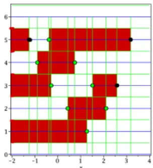
In the Budan table we present the roots and signs of f (x) and its derivatives for all x ∈ R as an infinite rectangle, formed by n + 1 bands (also called rows) R × [j − 0.5, j + 0.5[ with 0 ≤ j ≤ n. A root a of f(n−j) is represented by a bar
| positioned at a in the j-th band. between the bars | the sign of f(n−j)is fixed, if it is − the bloc is colored, if it is +
it remains white. In the picture we often put a small disk at the roots to point them out, sometimes the colors distin-guish the real roots from the non real ones. Consider figure 2, which shows the Budan table of a degree-6-polynnomial f without real roots. The black disks show the tree pairs of virtual roots of f .
The following arguments make it easy to determine the vir-tual roots in a given Budan table. First, we characterize the behavior of vmultf(a) and rmultf(a) when integrating f0:
Proposition 2.7. Let f ∈ R[X] monic, a ∈ R. Provided as well vmultf(a) − rmultf(a) as vmultf0(a) − rmultf0(a)
being even the following cases and only them can appear:
1. rmultf(a) = 0 = rmultf0(a) and
vmultf(a) = vmultf0(a);
2. rmultf(a) = rmultf0(a) + 1 and
vmultf(a) = vmultf0(a) + 1;
3. rmultf(a) = 0 < rmultf0(a) and
vmultf(a) − vmultf0(a) ∈ {−1, 0, 1}.
Proof. This follows form the definitons and correspond-ing examples.
This leads to the following way to determine if a real root of a derivative of f is a pair of virtual roots of f :
Proposition 2.8. Let f ∈ R[X] monic, a ∈ R. Let m be the number of 0 < i < n for which the following holds:
f(i)(a) = 0 and it exists an ² > 0 such that
f(i−1)(y)f(i)(y) > 0
f(i)(x)f(i)(y) < 0
f(i+1)(y)f(i)(y) > 0
for every x ∈]a − ², a[ and y ∈]a, a + ²[. Then
vmultf(a) =
(
2m if f (a) 6= 0, 2m + 1 if f (a) = 0.
Proof. This follows by induction on the degree and propo-sition 2.7.
3. GENERICITY AND RANDOMNESS
To simplify our analysis, we now on restrict to generic cases. Genericity is a concept used in algebraic geometry. Often in computer algebra, to choose a generic element we rely on the random function rand(), which produces numbers uniformly distributed in an interval. However, the two notions should not be confused.
3.1 Genericity
The set of degree n polynomials form a real vector space endowed with two natural topologies. The usual inherited form that of R and the Zariski topology. In the second one a basis of closed sets is formed by algebraic hypersurfaces defined as the zeros of multivariate polynomials. A property is then said generic if it is satisfied by a Zariski-dense subset of polynomials.
In practice, we try to concentrate all the ”bad“ behaviors that we want to avoid into an algebraic hypersurface (which need not be explicitly computed) and then just say ”generi-cally“. For instance all roots of the iterated derivatives of a generically given polynomial are two by two distinct.
Proposition 1. For a generic polynomial, all virtual not real roots are double.
Proof. As all roots of its iterated derivatives are 2 by 2 distinct, near such a root y of a derivative f(i) there is
small positive number e and an interval [y − e, y + e] where all the other derivatives keep a constant sign. So the only possibility for a sign variation between y − e and y + e is 0 or 2.
For a generic polynomial f , we can use Maple to pointplot the roots of the derivatives together with vertical lines pass-ing by them, as illustrated in Figure 2 with a polynomial of degree 6 having no real root. So we expect 3 double virtual roots. In order to locate these 3 virtual roots, we need to evaluate the signs of the derivatives on each row. We know that all the signs are + at ∞ and alternated + and − at −∞. Since the signs change at each root, the signs in the Budan table can be easily completed. Therefore, we can apply the discussion we made in section 2 of the characteri-zation of the patterns appearing in Budan table at a virtual
Figure 2: Blocs and roots
root. Then, a FDcurve or a stem of f (see below in the next section) can be used to express the propagation of the signs of the derivatives in a 2D picture. Let’s now state our main connexity result.
Theorem 3.1. Let f be generic monic univariate poly-nomial of degree n. The Budan table of f is represented by n + 1 bands of height one R × [i − 1/2, i + 1/2[ for i from 0 to n. A rectangle (possibly infinite) corresponding to negative values of a derivative is colored, while one corresponding to positive values remain white. The first band is white. Then:
• In this table, the number of connected colored compo-nents bounded on the right plus the number of con-nected white components bounded on the right equal the number of pairs of virtual non real roots plus the number of real roots.
• The rightest blocs of such a connected (bounded on the right) components, not on the n-th band, character-ize the virtual non real roots. The row of such a bloc indicates the degree of a derivative vanishing at the corresponding virtual root.
• Replacing f by −f , exchange the colors of the blocs, and rightest by leftest.
Proof. By genericity, we have n = 2m + p where p is the number of real roots and m the number of (double) virtual non real roots. On the n-th band there are q := dp/2e (negative) colored blocs bounded on the right and p − q (positive) white blocs bounded on the right. These p blocs are connected to one of the n infinite left, colored or white, ends (corresponding to the signs of the derivatives at −∞). By Rolle theorem and genericity, there are an odd number of roots on a row Li−1between two successive roots x1and x2
on Li. Two colored blocs on successive bands are connected
either on the right or on the left. By the discussion we made in section 2, only connection on the left is allowed when there is a single root on Li−1between x1 and x2, and
this configuration does not give rise to a virtual root. While when there are more than 2r + 1 roots between x1 and x2,
r pairs of virtual roots appear. The corresponding blocs are the end of two blocs components connected to the left (down) side of the table. Notice that such a virtual root
corresponds to the right side of a colored bloc (resp white bloc) but is surrounded by two white (resp. colored) blocs components coming from −∞. Hence 2m among the n ends at −∞ arrive at such points. The count is complete. The claim follows from this description.
Figure 2 illustrates an example of degree 6 with 3 virtual non real roots of multiplicity 2. There are 3 ”connected colored components bounded on the right“ and 0 ”connected white components bounded on the right“. They characterize 2 virtual roots on the 5-th row and a virtual root on the 3-rd row. See also the example at the end of the paper, where the situation is less simple.
3.2 Randomness
We call random polynomial, a polynomial whose coefficients are obtained by a random distribution, in general image of a classical law (Normal, uniform, Bernouilli). Two kinds of random polynomials have been extensively studied. First, those obtained by choosing a basis of degree n polynomials (xi or p1/i!xi, etc..) and taking linear combination with
random independent coefficients distributed with a classi-cal law. Second, the characteristic polynomials of random matrices whose entries are distributed with a classical law. A random polynomial f is, with a good probability, generic in the previous algebraic sens; but it is more specific. Indeed, its virtual roots inherit other statistical properties from the distribution of the coefficients of f ; when the degree n tends to infinity, some properties are asymptotically almost sure. For instance, generically the n complex roots of a polyno-mial are 2 by 2 distinct. But if we consider the characteristic polynomial of a dense random (128, 128) matrix, whose en-tries are instances of independent centered normal variables with variance v, its complex roots (the eigenvalues) are al-most uniformly distributed in a disk of radius √nv. This behavior is obviously not generic.
For large degree n (say 100), colored Budan tables look like discretized shapes, exploring this interpretation, it seems worthwile to also consider the derivation orders as discretized values, hence consider fractional derivatives.
4. FRACTIONAL DERIVATIVES
The idea to introduce and compute with derivatives or an-tiderivatives of non-integer orders goes back to Leibnitz. In the book [12], the authors relate the history of this concept from 1695 to 1975, the progression is illustrated by historical notes and they included more than a hundred enlightening citations from papers of several great mathematicians: Eu-ler, Lagrange, Laplace, Fourier, Abel, Liouville, Riemann, and many more.
In 1832 Liouville expanded functions in series of exponen-tials and defined q-th derivatives of such a series by oper-ating term-by-term for q a real number, although Riemann proposed another approach via a definite integral. They give rise to an integral of fractional order called Riemann-Liouville integral for q < 0, which depends upon an origin a and generalizes the classical formula for iterated
integra-tions: [ d qf [d(x − a)]q]R−L:= 1 Γ(−q) Z x a [x − y]−q−1f (y)dy. Then for positive order and any sufficiently derivable func-tion f , one relies on a composifunc-tion property with dm
d(x−a)m,
for an integer m. So, for any real number m+q, one obtains: [ d m+qf [d(x − a)]m+q]R−L:= dm d(x − a)m[ dqf [d(x − a)]q]R−L].
Thanks to properties of the Γ function, this definition is coherent when a change of (q, m) keeping m + q constant. The generalization of this definition to other functions f . is discussed in the book [12]. The traditional adjective “frac-tional“ corresponding to the order of derivation is mislead-ing, since it need not be rational.
Let us emphasize that nowadays in mathematics, fractional derivatives are mostly used for the study of PDE in func-tional analysis. They are presented via Fourier or Laplace transforms. Fractional derivatives are seldom encountered in polynomial algebra or in computer algebra. The second author learned this concept and its history working on [10], then used the following very simple formula, with q > 0 and n an integer, attributed to Peacock.
dq [d(x − a)]q(x − a) n := n! (n − q)!(x − a) n−q .
We illustrate it with the monomials of a polynomial, q = 1 2 and a = 0: d1/2 [dx]1/2(x 2− 2x + 3, x) = (8 3x 2− 4x + 3)x−1/2√1 π.
4.1 A bivariate polynomial
Lemma 1. Let f (x) be a polynomial of degree n, then (x − a)qΓ(−q) d
qf
[d(x − a)]q
is a polynomial in x and q.
To interpolate the non vanishing roots of the successive derivatives of a polynomial f , only fractional derivatives, up to a power of (x − a) are needed. We introduce the fol-lowing notations for a family of univariate polynomials in q and another in t := n − q, indexed by their degrees. Notations: For i = 0, ..., n − 1, l0:= 1; ln−i(q) := n Y j=i+1 1 −q j; λ0:= n!;
λn−i(t) := n!ln−i(n − t) = i!t(t − 1)...(t + i + 1 − n).
Definition 1. Let f =Pai(x − a)i be a degree n
poly-nomial. We call monic polynomial factor of a fractional derivative of order q, with respect to the origin a, of f ,the
Figure 3: A simple FDcurve
bivariate polynomial (x − a)q (n−q)! n!
dqf
[d(x−a)]q. It is a
polyno-mial of total degree n in (x − a) and q which writes
n−1
X
i=0
ai(x − a)iln−i(q).
It will be convenient to let t = n − q, and consider the poly-nomial obtained with this substitution:
Pf(x, t) := 1 n! n X i=0 ai(x − a)iλn−i(t).
For all k = 0, ..., n, we have Pf(x, n−k) =(n−k)!n! (x−a)kf(k).
It also holds (x − a)∂
∂xPf = P(x−a)f0.
The previous bivariate polynomial realizes an homotopy be-tween the graphs of f (x) and (x − a)f0(x) when q varies
between 0 and 1.
4.2 FDcurve
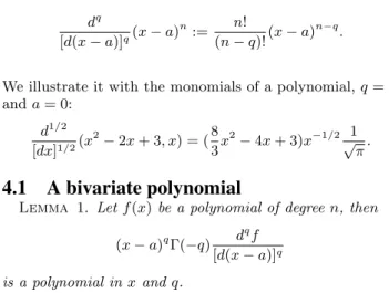
Definition 2. We call FDcurve, with origin a, of a poly-nomial f of degree n, the real algebraic curve defined by the bivariate equation Pf(x, t) = 0.
Notice that instead of taking the origin at a, we can fix the origin at 0, perform a substitution x := x − a on f and then translate the obtained curve.
Figure 3 shows a simple example with f := (x − 1)(x − 2)(x − 3)(x − 4)(x − 5)(x − 6), n = 4, a = 0, an hyperbolic polynomial, hence all its derivatives are hyperbolic. The roots of f and its derivatives are represented by small green disks. In Figure 4 we first performed a substitution with a = 3.5. The two curves are quite different, the second has 3 connected components and infinite branches, but both pass through all the roots. The FDcurve corresponding to other values a may have singularities (e.g. double points). So the topologies of the FDcurve can change with a.
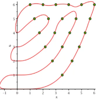
In many examples all the connected components cut the axis x = a, but it is not always the case: Figure 5 shows the small lonesome component of the example, with a = 0,
f = x6+10.4x5+34.55x4+41.20x3+29.85x2−15.00x−0.37.
However no root lies on this small component, we do not know if it is always so. In this example f has two real roots,
Figure 4: Changing the origin a
Figure 5: A lonesome component
it has also two virtual double roots, their location will be studied in the next section.
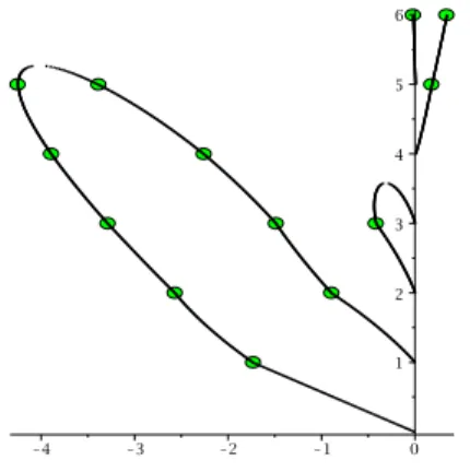
In [10], another curve (an algebraic C0 spline), called the
stem of f , is associated to a degree n polynomial f . It is defined as the union of the real curves formed by the roots of all the monic polynomial factors of the derivatives f(i)of f ,
for i from 0 to n − 1 and 0 ≤ q < 1. Stems were designed to study the roots of the derivatives of random polynomials of high degrees and exploit their symmetries. To illustrate the differences between these two constructions, Figure 6 shows the stem corresponding to the previous FDcurve with the lonesome component: it is less curved.
5. LOCATION OF VIRTUAL ROOTS
For f a generic monic univariate polynomial of degree n, in this section, we consider partitions of the infinite rect-angle R. R is the union of n + 1 bands of height one R × [i − 1/2, i + 1/2[ for i from 0 to n. In the previous sec-tion, we have seen the partition of R corresponding to the Budan table: the rectangles (possibly infinite) correspond-ing to negative values of a derivative are colored while the ones corresponding to positive values remain white. Theo-rem 3.1 shows that this partition allows to locate the virtual roots of f . Here, we aim to rely on the ovals of FDcurves or stems to transmit ”quickly“ the sign information needed for the partition of the Budan table.
For this purpose, let us consider an example where all the roots of the derivatives of f are positive, and choose a = 0.
Figure 6: Stem of the previous curve
Figure 7: Budan inside and around an FDcurve
This is always possible up to a translation on x. We take the intersection of the negative part of the Budan table and the negative locus of Pf (delimited by the components of the
FDcurve). In Figure 7 the intersection zones are colored in grey. These intersection zones are helpful to see that some blocs are connected but not sufficient to guaranty that other blocs are disconnected. So, we also consider the zones col-ored in blue, shaped as curved triangles in the picture. Two blue zones attached to two separated connected components of the FDcurve may intersect, this happens in Figure 8 with the same example where we changed the origin a, hence the FDcurve. Let’s do the same constructions with the stem of Figure 6. In that case, the interiors of the ovals correspond to positive values of an implicit function, so it is better to color the positive blocs. Now, the virtual roots correspond to the leftest blocs. This is illustrated in Figure 9: the 2 virtual roots are immediately located at the leftest roots on the two left ovals.
As a conclusion, we can say that depending on the shape of the stem of f or of an FDcurve, the location of the virtual roots may become very fast. But this possibility should be studied case by case.
5.1 An example of medium degree
We consider a randomly generated polynomial of degree n = 16, taking a random linear combination of the so-called
Figure 8: Connecting the components
Figure 10: Collapsing blocs
Bernstein polynomials, used in Computer Aided Design. It has 6 real roots. In Figure 10, we truncated the picture, and we see only 4 of them. So it remains 5 double virtual roots. In the picture real roots and virtual roots are repre-sented by blue disks. We colored in grey the positive blocs. Among the 5 virtual roots, 4 correspond to grey blocs com-ponents and 1 to a white blocs component.
Notice that the FDcurve is helpful for locating the posi-tive virtual roots (at the end of the ear shaped curves), but not for the negative virtual roots. Therefore it is useful to reduce to positive values and simultaneously consider the polynomial obtained by changing f (x) into (−1)nf (−x).
6. CONCLUSION
We characterized the possible patterns between successive rows in a Budan table corresponding to a virtual roots. Re-stricting to the generic case we gave a global characterization (using connectivity of connected components) of the loca-tion of virtual roots in a Budan table. In addiloca-tion, we used fractional derivatives to associate a bivariate polynomial to f , and introduced two types of plane curve associated to f , which help geometrically see the signs taken by the iterated derivatives of f hence locate, in many cases, a virtual roots near one of their critical points. We suggest three directions for future researches:
• Investigate what happens when we relax the generic-ity hypothesis (i.e. specialization to more degenerated cases),
• Study the relationship beteen virtual roots in an inter-val and pairs of conjugate complex roots which lie in a sector close to this interval counted by Obreschkoff theorem, see [13], chapter 10.
• generalize to other families of functions beyond the polynomials, as initiated in [6].
Acknowledgments
We are grateful to Henri Lombardi for valuable discussions. Andr´e Galligo was partially supported by the European ITN Marie Curie network SAGA. Daniel Bemb´e was partially supported by the Deutsch-Franz¨osische-Hochschule ´ Ecole-Franco-Allemande.
7. REFERENCES
[1] Akritas Alkiviadis G., Reflections on an pair of theorems by Budan and Fourier, University of Cansas 22.
[2] Bemb´e, D: Budan’s theorem and virtual roots of real polynomials Preprint.(2009)
[3] Bharucha-Reid, A. T. and Sambandham, M.: Random Polynomials. Academic Press, N.Y. (1986).
[4] Bochnack, J. and Coste, M. and Roy, M-F.: Real Algebraic Geometry. Springer (1998).
[5] Budan de Boislaurent, Nouvelle m´ethode pour la r´esolution des ´equations num´eriques d’un degr´e quelconque. Paris (1822). Contains in the appendix a proof of Budan’s theorem edited by the Acad´emie des Sciences (1811).
[6] Coste, M and Lajous, T and Lombardi, H and Roy, M-F : Generalized Budan-Fourier theorem and virtual roots. Journal of Complexity, 21, 478-486 (2005). [7] Edelman,A and Kostlan,E: How many zeros of a
random polynomial are real? Bulletin AMS, 32(1):137, (1995).
[8] Emiris, I and Galligo, A and Tsigaridas, E: Random polynomials and expected complexity of bissection methods for real solving. Proceedings of the
ISSAC’2010 conference, pp 235-242, ACM NY, (2010). [9] Farahmand,K: Topics in random polynomials. Pitman
research notes in mathematics series 393, Addison Wesley, (1998).
[10] Galligo, A: Intriguing Patterns in the Roots of the Derivatives of some Random Polynomials. Submitted (2010).
[11] Gonzales-Vega, L and Lombardi, H and Mah´e, L : Virtual roots of real polynomials. J. Pure Appl. Algebra,124, pp 147-166,(1998).
[12] Oldham, K and Spanier, J: The fractional calculus. Academic Press Inc. NY, (1974).
[13] Rahman, Q.I and Schmeisser,G: Analytic theory of polynomials, Oxford Univ. press. (2002).
[14] Vincent M,. Sur la r´esolution des ´equations num´ericques, Journal de math´ematicques pures et appliqu´ees 44 (1836) 235–372.