A summary of the Planck constant determinations using the NRC Kibble balance

Publisher’s version / Version de l'éditeur:

Metrologia, 54, 3, pp. 399-409, 2017-05-30

READ THESE TERMS AND CONDITIONS CAREFULLY BEFORE USING THIS WEBSITE. https://nrc-publications.canada.ca/eng/copyright

Vous avez des questions? Nous pouvons vous aider. Pour communiquer directement avec un auteur, consultez la première page de la revue dans laquelle son article a été publié afin de trouver ses coordonnées. Si vous n’arrivez pas à les repérer, communiquez avec nous à PublicationsArchive-ArchivesPublications@nrc-cnrc.gc.ca.

Questions? Contact the NRC Publications Archive team at

PublicationsArchive-ArchivesPublications@nrc-cnrc.gc.ca. If you wish to email the authors directly, please see the first page of the publication for their contact information.

NRC Publications Archive

Archives des publications du CNRC

This publication could be one of several versions: author’s original, accepted manuscript or the publisher’s version. / La version de cette publication peut être l’une des suivantes : la version prépublication de l’auteur, la version acceptée du manuscrit ou la version de l’éditeur.

For the publisher’s version, please access the DOI link below./ Pour consulter la version de l’éditeur, utilisez le lien DOI ci-dessous.

https://doi.org/10.1088/1681-7575/aa70bf

Access and use of this website and the material on it are subject to the Terms and Conditions set forth at

A summary of the Planck constant determinations using the NRC

Kibble balance

Wood, B. M.; Sanchez, C. A.; Green, R. G.; Liard, J. O.

https://publications-cnrc.canada.ca/fra/droits

L’accès à ce site Web et l’utilisation de son contenu sont assujettis aux conditions présentées dans le site LISEZ CES CONDITIONS ATTENTIVEMENT AVANT D’UTILISER CE SITE WEB.

NRC Publications Record / Notice d'Archives des publications de CNRC:

1. Introduction

It is expected that the world’s measurement system, the SI, will soon be revised with seven deining constants at its foundation [1]. In preparation for this event the CODATA Task Group on Fundamental Constants has requested that laboratories performing high accuracy determinations of these constants, in particular the Planck, Avogadro and Boltzmann constants, submit their latest results by July 1, 2017 [2, 3]. These and previous results will be used to establish the ixed values for the constants to be ultimately recommended to International Committee on Weights and Measures (CIPM) and then used in the revised SI [4].

In 2014 we published four watt balance results [5, 6], each associated with a different test mass, which represented the most precise Planck constant determination at that time. These were the result of a few years of effort resolving major issues of the previous NPL watt balance including mass exchange errors [7], coil suspension and alignment [8]. Since that time the balance has been disassembled, primarily to modify the tare mass lift and to make modiications to the interferom-eter. The resulting improvements have been used in three new determinations: the irst performed in February 2016 with a silicon 500 g mass, the second in November 2016 with a gold-plated copper (AuCu) mass of 1 kg and the third in December 2016 with a AuCu 500 g mass.

The original four determinations were reanalysed including new corrections, and complete re-evaluations of their uncertainty budgets were made using the results of new auxiliary tests. The three new determinations were similarly analysed. There are signiicant correlations between these

A summary of the Planck constant

determinations using the NRC

Kibble balance

B M Wood, C A Sanchez, R G Green and J O Liard

National Research Council of Canada, 1200 Montreal Road, Ottawa, ON K1A 0R6, Canada

E-mail: barry.wood@nrc-cnrc.gc.ca

Received 31 March 2017, revised 28 April 2017 Accepted for publication 3 May 2017

Published 30 May 2017

Abstract

We present a summary of the Planck constant determinations using the NRC watt balance, now referred to as the NRC Kibble balance. The summary includes a reanalysis of the four determinations performed in late 2013, as well as three new determinations performed in 2016. We also present a number of improvements and modiications to the experiment resulting in lower noise and an improved uncertainty analysis. As well, we present a

systematic error that had been previously unrecognized and we have quantiied its correction. The seven determinations, using three different nominal masses and two different materials, are reanalysed in a manner consistent with that used by the CODATA Task Group on Fundamental Constants (TGFC) and includes a comprehensive assessment of correlations. The result is a Planck constant of 6.626 070 133(60) ×10−34 Js and an inferred value of the Avogadro constant of 6.022 140 772(55) ×1023 mol−1. These fractional uncertainties of less than 10−8 are the smallest published to date.

Keywords: kilogram, watt balance, redeinition, Kibble balance, Planck constant, mass measurement

(Some igures may appear in colour only in the online journal)

Original content from this work may be used under the terms of the Creative Commons Attribution 3.0 licence. Any further distribution of this work must maintain attribution to the author(s) and the title of the work, journal citation and DOI.

https://doi.org/10.1088/1681-7575/aa70bf

seven determinations and they must be taken into account to not underestimate the overall uncertainty. In general this is a rather dificult task for the CODATA TGFC to perform because the critical information is usually not available or not presented in a consistent manner. In fact for determinations made within the same laboratory the authors themselves are the source of such information and it is optimal for them to make this assessment in a transparent fashion.

The use of the term ‘Kibble balance’ has been endorsed by the CCU/CIPM [9] in recognition of the contributions of the late Bryan Kibble to metrology and in particular for con-ceiving the concepts of the watt balance. The NRC watt bal-ance project especially recognizes this contribution because we have beneited from the design and construction of both Bryan Kibble and Ian Robinson. The Kibble or watt balance has been well described before [5, 10] and the following is only a supericial outline.

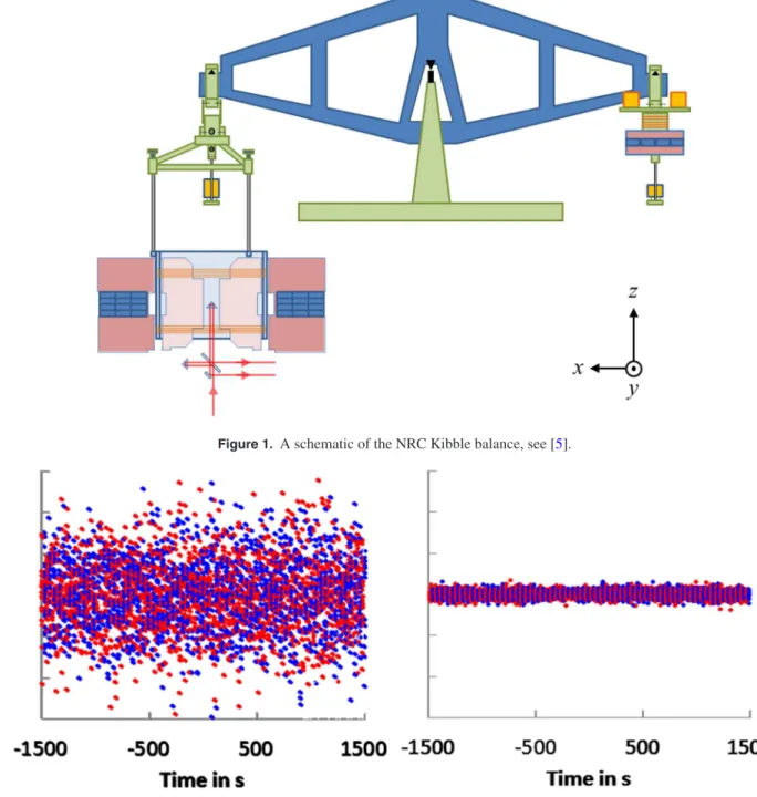
The NRC watt balance consists of a classic equal arm beam balance with a test mass, coil and radial magnetic ield on one side and a counter balancing tare mass on the other side; see igure 1. With the tare and test masses raised and zero current through the coil the beam is approximately bal-anced. An interferometer measures the position and velocity of the coil.

In the weighing phase the interferometer controls a feed-back current which passes through the coil and generates a force to balance the beam. The general force equation is

= =

F mg BL I

(1) where F is the force, m is the test mass, g is the acceleration due to gravity, BL is the integrated cross product of the magn-etic lux density and the coil length and I is the coil current.

In the moving phase both the tare mass and test mass are raised and the balanced beam is moved by a voice coil on the tare side of the balance. The interferometer controls a feed-back current which now passes through the voice coil and produces a constant coil velocity. The resulting coil voltage is described by:

=

V  v BL

(2) where V is the coil voltage and v is the coil velocity.

Assuming that BL is the same in the weighing and moving phases then

/υ =

mg IV

(3) This relationship is now called the Kibble equation. If we measure the current I by measuring the voltage VI developed across a resistor R and use the Josephson and quantum Hall effects and their conventional 1990 values as the reference for the voltage and resistance measurements we get

= ×

h mgv VI h90

(4) where h90 is related to the Josephson and quantum Hall effect conventional values   = − − h K R 4 J K 90 90 2 90 (5) 2. Improvements 2.1. Tare mass lift

In 2012 the NRC watt balance mass exchange errors [7] were detailed. The largest of these errors was caused by a tilting of the balance platform during the mass exchange and it was elimi-nated by moving the mass lift off the platform and onto the base. The tare lift was also mounted on the balance platform and it also caused a platform tilt but since the tare mass remains on during the entire weighing phase it did not introduce an error that is synchronous with the main mass status. However, lowering the tare mass does cause a small displacement and tilting of the coil, with respect to the coil’s position in the moving phase, and this had been assessed as a 3 × 10−9 _{type B relative uncertainty.}

The balance itself was disassembled so that the tare mass lift could be moved off the balance platform and onto the base. It was hoped that this modiication would completely eliminate the coil displacement but a small residual coil shift remains, probably due to loading distortions of the lexure and knife edge pivots.

2.2. Interferometer noise reduction

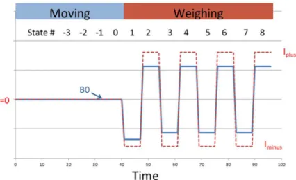
Before 2014 the measurements of BL in the moving phase showed a typical relative scatter of about 60 × 10−9, a level of noise which is signiicantly higher than that in the weighing phase and also higher than can be expected from the instrumentation. Fourier analysis of the separate voltage and velocity signals, as well as their ratio, provided clear evidence that the excess noise originated from sharp resonances in the velocity measurement occurring below 200 Hz. The reso-nant frequencies were relatively stable and their amplitudes drifted slowly over days but usually increased. Many possible causes such as electrical interference, coil vibration modes, acoustically coupled vibration, laser output characteristics (spectral purity, amplitude, polarization and pointing stability) were considered and tested but failed to indicate the cause. Eventually the problem was traced to the beam splitter of the Michaelson interferometer which was mounted in such a way that the beam splitter was distorted and strained.

A mild distortion of the beam splitter caused the interfer-ence pattern to vary over a fraction of a fringe. Remounting the beam splitter with minimal distortion improved the uni-formity of the interference pattern and increased the optical contrast but also caused the sharp resonances to disappear.

We believe that the resonances were caused by strain induced vibrational modes of the beam splitter in vacuum. The reduction in noise of the moving phase is substantial, almost a factor of ten as seen in igure 2. Measurements over the last two years conirm that the improvement is permanent.

2.3. Local ield compensation

With this reduced noise in the moving phase we were now able to clearly observe and correct for the local environmental magnetic lux density. The voltage induced across the coil responds to the total lux density in the gap which includes the Metrologia 54 (2017) 399

large, slowly varying lux produced by the magnet, as well as a contribution from the much smaller local lux which can vary quickly and randomly on the time scale of these measurements. The local lux density is measured independently with a con-ventional magnetometer. The strength of the coupling into the gap was determined by itting the data during a large amplitude variation of the local ield. A local ield to gap ield sensitivity of 1.2 T/T has been measured. Removing the local lux contrib-ution from the moving data improves the itting of the slowly varying portion of BL. The weighing data then utilizes this low frequency value of BL combined with the local lux during the weighing phase to calculate an equivalent mass. Reductions in the uncertainty of the measured mass of up to 40% have been observed when the local ield varies considerably.

2.4. Magnetization

Whenever current passes through the coil, magnetization of the material closest to the coil, usually part of the yoke, is inevitable. This process has been considered before [5, 10, 11] and is commonly modelled as a current dependence of the lux density in the gap,

 ( α  β )

= + +

B B0 1 I I2

(6) where B0 is the lux density in the gap with zero current in the coil and α and β are the fractional coeficients related to the irst and second order current dependence.

In the weighing phase two states are involved, both with the tare mass lowered. The irst state has the mass off the pan and Figure 1. A schematic of the NRC Kibble balance, see [5].

Figure 2. The residuals of the moving phase data illustrating the noise reduction. On the left a typical data set from 2013 with the slightly distorted beam splitter. On the right a data set after removing the beam splitter strain. The vertical and horizontal scales of both data sets are the same.

an associated coil current Ioff. The second state has the mass on the pan and an associated current, Ion ≈ −Ioff. Using the Kibble equation it can be shown that the error due to the irst order magnetization term is given by α(Ion + Ioff). Previously, we have determined the irst order fractional dependence,

α = 0.56 × 10−6 _mA−1_{. This is done by weighing with} var-ious beam or tare mass imbalances. The mean current of the Mass_On and Mass_Off states is typically kept very small with respect to the nominal current and the fractional error is ~1 × 10−8 _{before correction.}

Determination of the second order term, β, has been more dificult. To date we have not managed to get consistent determinations of β within their estimated uncertainties using asymmetric weighing. However, an upper bound of the second order coeficient is set by the differences in Planck constant determination values using different nominal masses (i.e. 1 kg and 0.5 kg). This estimate was previously used as an uncertainty component of the second order effect [5] and has been reconsidered with new data that shows (h1 kg − h0.5 kg)/

h1 kg = −0.01 × 10−9_{. This would suggest that the upper limit} of this error is <0.013 × 10−9 _{for the 1 kg results. We remain} uneasy about this estimate. In the end we have accepted an upper bound estimate of the β uncertainty based on the uncer-tainty of the difference of the 1 kg and 500 g results which is 3.94 × 10−9_{. This suggests | β | < 0.0205 × 10}−9 _mA−2 _and corresponds to 5.3 × 10−9_{, 1.3 × 10}−9 _{and 0.3 × 10}−9 uncer-tainty components for the1 kg, 500 g and 250 g results.

It is important to note that for this system, current induced magnetization is predominately a linear process because the ratio of the effects of the linear to second order magnetization is about 0.001 .

Another effect, magnetic hysteresis, is well known to exist but quite complicated to model, especially in this situation and at these levels [10–13]. To understand the nature of this error it is necessary to consider the coil current states of our watt balance experiment and some generic properties of the hysteretic processes. Hysteresis describes any process which ‘lags behind’ and is typically identiied as a parameter con-trolled system which starts from an initial state, changes as the driving parameter changes but does not return to the initial

state even though the driving parameter has returned to its ini-tial value. Let us consider an extremely simplistic hysteresis model in which the magnetic state, Bi, is a function of the coil current and the difference between the previous state and pre-sent state, Bi = B0(1 + αI + βI2) − γ(Bi − Bi−1).

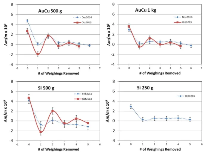
In our watt balance experiment the coil current states can be thought of as a number of zero-current states, representing the moving phase of the experiment, followed by successive

Iminus and Iplus coil current states representing the weighing phase, see igure 3. If we arbitrarily make γ = 0.3 then the corresponding hysteresis effect can be observed as shown in igure 3.

In igure 3 the dashed red line indicates the coil cur-rent, through the moving phase with I = 0 and through the weighing phase with the alternating Iminus and Iplus states. The state index is above, with state 1 as the irst weighing state. The solid blue line is the magnetic state, equal to B0 through the moving phase and switching by several parts per million in the weighing phase due to the αI term. Although not shown in igure 3, at the end of the weighing phase and before the next moving phase, a demagnetizing process is performed. In this process the coil current oscillates in a decaying pattern by pushing against a mass held by the mass lift. This process effectively demagnetizes the effects caused by the weighing process and returns the magnet to the B0 state.

Note that the magnetic state 1 is smaller than magnetic states 3, 5 and 7. In this simplistic model, magnetic states 2, 4, 6, 8 are all equal. Secondly, note that the mean of states 7 and 8 equals B0. It turns out that these are general properties of all hysteretic processes driven by a linear function and for our watt balance they can be restated as:

• The weighing steady state is symmetric with respect to the moving steady state.

• The initial weighing states are the most affected by hysteresis but the effect decays with successive weighing states.

With this simplistic model only the irst weighing state dis-plays any hysteresis effect and it causes a positive mass error because mass is related to Iplus − Iminus in this substitution Figure 3. A schematic of the coil current (dashed red) and magnetic states (solid blue) of the watt balance measurements in the moving and weighing phases versus time in seconds.

measurement. Other models incorporating multiple states, time dependence etc tend to spread the effect to subsequent states. The initially positive mass error remains common.

At NRC to account for drift in the balance of the beam we analyse the weighing results with a linear regression, itting not only to the Mass_On and Mass_Off states but also to a irst and second order time dependence, Removing the irst and second order time dependence from data which exhibits hysteresis complicates the interpretation of the hysteresis effect but it does not affect the interpretation of the steady state solution.

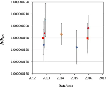
Fortunately, a simple but computationally intensive tech-nique can reveal the hysteresis effect with good precision and without additional measurements. The watt balance data is reanalysed, successively removing the initial weighing state data until only three weighing states remain, suficient to establish the beam drift components. This is done for the several hundred weighing sequences of each Planck determi-nation. The result is a histogram of mass changes caused by the removal of different numbers of initial weighing states, see igure 4. The noise or scatter of this process is very small because of the large size of the data.

Despite our very non-speciic model the plots conirm several aspects.

• The initial mass deviation is always positive.

• The mass deviation decays within a few weighing states, and then becomes stable and repeatable.

• The noise is small; the scatter of the steady state relative mass deviations is ~0.8 × 10−9_.

The few negative points in igure 4 are believed to be caused by the inluence of the irst and second order time dependence of the beam drift.

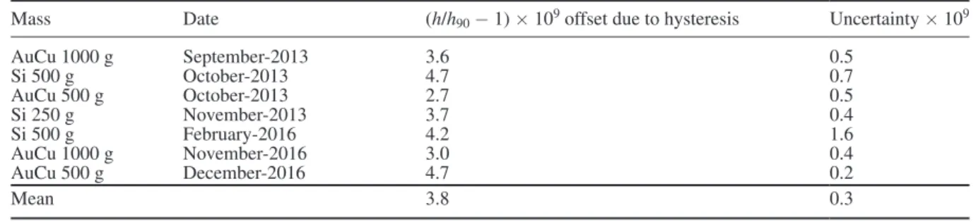
The effect of hysteresis on each Planck constant deter-mination can be assessed as the difference of the analysis with no weighing states removed and the analysis of the steady state solution, see table 1. This is very consistent, (3.8 ± 0.8) × 10−9_{, when expressed as a fractional part of the} measured mass and thus is dependent on mass and not mass squared. However, we think that the hysteresis effect should also be dependent on the coil position within the magnetic gap and this can vary with the realignment of each Planck determination. For this reason each Planck determination was corrected by its own hysteresis evaluation.

It must be noted that hysteresis does not have to be magn-etic in origin. Similar effects can occur with mechanical hys-teresis of the knife edges and lexures. Fortunately, the very general hysteresis principles are still applicable and the steady state solution remains valid.

The power heating of the resistor was considered during the process of removing and reanalyzing weighing data. The drift of the resistance due to self-heating has been sepa-rately evaluated by calibrating the resistor directly against the quantum Hall standard at the highest currents used, those associated with the 1 kg test mass. These indicate Figure 4. The hysteresis plots of the seven Planck determinations.

a correction of about 1 × 10−9 _{versus the simple average} resistance of the calibration.

2.5. Synchronization

The moving phase determines BL by measuring the voltage to velocity ratio. Optimum signal to noise can be achieved through three techniques

• Having the voltage and velocity as constant as possible • Reducing the high frequency content of both signals as

much as possible

• Simultaneous data acquisition of the voltage and velocity signals

We have measured the effect of desynchronization by making moving phase measurements and alternating the amount of desynchronization by synchronizing the beginning of the voltage and velocity data acquisition but intentionally retarding the completion of the voltage acquisition. The successive dif-ferences of BL are not sensitive to the drifting value of BL and the increasing uncertainty of BL is used as an indicator of the effect of desynchronization. With this technique, our typical 10 µs of synchronization error in a 0.4 s sample causes 0.6 × 10−9 of itting uncertainty in the determination of BL. This sets an upper limit of the desynchronization error in our measurements.

2.6. Velocity dependence

All of our seven Planck constant determinations have been performed with a moving phase velocity of 2 mm s−1. It is important to establish if the BL determinations are

independent of velocity. This independence of the moving phase has been re-evaluated at 2 mm s−1_{, 1 mm s}−1 _and 0.5 mm s−1_{. A weighted it of the relative differences of BL} versus velocity has been made which when extrapolated to 0 mm s−1 _{gives a correction of (1.0 ± 2.6) × 10}−9 _{for the} 2 mm s−1 _data.

Figure 5. The re-pooled data, 24 h averages, of each of these three determinations is shown. The uncertainties are the type A uncertainties of the re-pooled data sets. Vertical axis is plotted as (h/h90 − 1) × 109 which is mass independent and more clearly shows the deviations on a common scale. The orange data point is the dataset mean. The horizontal scales for the three plots are in days but are not identically spaced.

Figure 6. A plot of the seven Planck constant determinations versus time. The red square data points are made with 1000 g AuCu, the blue circle data points with 500 g Si, the red triangle data points with 500 AuCu and the small blue circle data point with 250 g. The uncertainty bars represent the combination of re-pooled standard deviation of the mean, root-sum-squared with the determination’s uncertainty budget but with no account for correlations. The single gold point represents the inverse covariance weighted mean and its uncertainty bars do account for correlations.

2.7. Miscellaneous

The intensities of the optical signals of the homodyne interfer-ometer have been balanced so that the interference amplitude has improved long term stability. The shielding of the inter-ferometer electronics was improved to further reduce interfer-ence from other high frequency signals. A small vacuum leak which became evident in the middle of the 2013 campaign has been found and repaired.

3. The 2014 data set re-analysis

The four 2014 data sets were completely reanalysed. The 35 × 10−9 correction for the 2014 mass traceability to the IPK due to a revision of the BIPM mass scale was applied

with a revised uncertainty [6] and the previously described hysteresis corrections and their uncertainties were applied. A very minor correction for pressure was applied to deter-minations #3 and #4 to correct for the recalibration of our vacuum gauge.

A data set for each Planck value determination consists of 112 to 190 alternating weighing and moving sequences each taking approximately 45 min. The itting of neighbouring data from sets of three moving sequences establishes the BL values used to analyse the data of each weighing sequence. Thus a different Planck value is obtained for each weighing sequence every 90 min. For the 2014 data sets, as well as the 2016 data sets (see table 2), the mean is taken as the simple mean of all the points in the data set (112–190 points). The data was then re-pooled into 24 h averages using a consistent method which Table 1. A table of the hysteretic offsets and uncertainties for our seven Planck constant determinations. The offsets are the change in (h/h90 − 1) × 109.

Mass Date (h/h90 − 1) × 109 offset due to hysteresis Uncertainty × 109

AuCu 1000 g September-2013 3.6 0.5 Si 500 g October-2013 4.7 0.7 AuCu 500 g October-2013 2.7 0.5 Si 250 g November-2013 3.7 0.4 Si 500 g February-2016 4.2 1.6 AuCu 1000 g November-2016 3.0 0.4 AuCu 500 g December-2016 4.7 0.2 Mean 3.8 0.3

Table 2. A summary of the conventional results of the seven Planck constant determinations showing the index, mass material, nominal mass in grams, the number of points and re-pooled points, the Planck constant values and their deviations and uncertainties in parts in 109. No accounting for the correlations has been made for these values.

# ID Grams # points # pooled points h/h90 (h/h90 − 1) × 109 Simple combined uncertainty × 109 1 AuCu 1000 143 16 1.000 000 190 190.04 14.0 2 Si 500 112 13 1.000 000 184 184.28 12.9 3 AuCu 500 156 17 1.000 000 194 194.05 12.6 4 Si 250 148 16 1.000 000 205 205.08 13.8 5 Si 500 150 10 1.000 000 182 182.19 14.2 6 AuCu 1000 156 12 1.000 000 190 189.55 12.4 7 AuCu 500 190 16 1.000 000 199 198.72 10.3

Table 4. The total covariance matrix of the seven determinations. The units of the table elements are relative uncertainty squared i.e. (uh/h90 × 109)2.

Total covariance matrix of the h/h90 × 109 determinations

201.87 129.93 130.16 114.59 60.82 82.32 61.45 129.93 174.47 124.09 115.57 57.81 60.89 57.22 130.16 124.09 193.44 115.25 57.65 60.77 57.18 114.59 115.57 115.25 227.00 59.61 57.02 59.39 60.82 57.81 57.65 59.61 205.02 66.56 60.42 82.32 60.89 60.77 57.02 66.56 157.21 83.59 61.45 57.22 57.18 59.39 60.42 83.59 111.58

Table 3. A summary of various averages of the seven Planck constant determinations showing the type of aggregate, the h/h90 value and the deviation and uncertainty in parts in 109. This table shows the increase in assessed uncertainty caused by accounting for correlations.

h/h90 (h/h90 − 1) × 109 Uncertainty × 109

Simple mean 1.000 000 192 191.99 3.03

Simple inverse total variance weighted mean 1.000 000 192 192.06 4.79 Inverse covariance weighted mean 1.000 000 193 192.97 9.15 Metrologia 54 (2017) 399

was used for the analyses of all of the determinations. The standard deviation of the mean of the re-pooled data set was then used as the Type A uncertainty of the mean value. This had the effect of reducing the degrees of freedom by a factor of about 11 (see table 3). The uncertainties were reviewed and the covariances with other determinations were established. 4. New Planck constant determinations

In February 2016 we measured a 500 g silicon mass and this was the irst determination to beneit from the interferometer noise reduction and local magnetic ield compensation. The type A noise and stability are noticeably improved. Because of the noise improvements, the moving and weighing sets are made approximately equal in time, each about 45 min and a mass result is obtained every 90 min. Again the mean is taken as the simple mean of all of the data while its Type A uncer-tainty is taken as the standard deviation of the mean of the re-pooled 24 h data set (see igure 5). This data set has inde-pendent resistance, laser and gravity determinations and has the least correlation with the other Planck determinations.

In November 2016 we measured a 1 kg AuCu mass and in December we measured a 500 g AuCu mass. Again the Type A noise and stability are improved. These data sets appear to be slightly degraded by vibration due to nearby construction. These two data sets have independent resistance calibrations but share, laser frequency and gravity determinations.

5. Covariant analysis

Table 2 shows the seven Planck constant determinations and their simple uncertainties comprised of the standard deviation of the mean of their 24 h averaged data combined with the 57 other components of each uncertainty budget. The data spans a period over three years and the relative standard deviation of the seven results is only 8.1 × 10−9. However there are correlations between the seven determinations and a proper covariant weighted mean must be calculated to not overesti-mate the degrees of freedom and not underestioveresti-mate the total combined uncertainty.

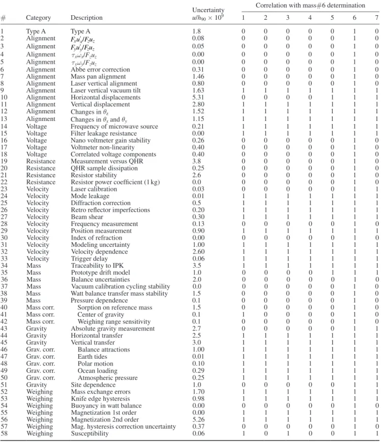
At the heart of any such analysis are the uncertainty budgets of the seven determinations. Appendix 1 shows the uncer-tainty budget of the 6th determination (1 kg AuCu, November 2016) and its correlations with all of the determinations. The derivation of the individual uncertainty components is usually self-evident from the description but the reader is directed to earlier reports [5, 7, 8, 14] which have described them in much more detail.

Consistent with the general analysis procedures of the CODATA TGFC we have calculated an inverse variance weighted mean and account for correlations by constructing a full covariance matrix. With seven determinations and 58 uncertainty components for each uncertainty budget, the total number of individual covariances become unmanageably large (7∗58∗7∗58 = 164 836). However, the common structure of the uncertainty budgets greatly reduces this number because we can assume that covariances between different types of

uncertainty components are zero. Thus only covariances between different determinations, but of the same type of uncertainty component, need be considered. Because covari-ances are additive we can add the 58, 7 × 7 covaricovari-ances asso-ciated with each uncertainty component to assemble the total covariance matrix. See appendix and table 4.

The inverse covariance weighted mean is h/h90 = 1.000 000 1930 and its uncertainty is 0.000 000 0091, see igure 6. The chi-squared is 4.4 and the Birge ratio is 0.85 . 6. Discussion of the results

Table 2 shows that the total uncertainties of the seven determi-nations are very similar despite the improvements in the Type A component of determinations 5, 6 and 7. In part this is a consequence of the uncertainty loors of the different catego-ries of uncertainty, see table 5. The following is a brief sum-mary of each category and possible improvements.

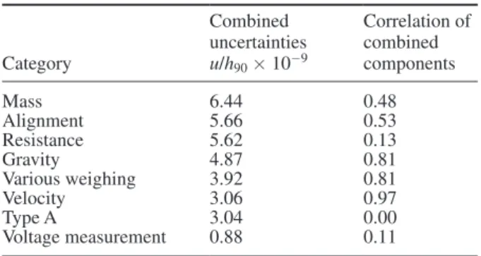
The mass uncertainty category has improved since 2014 and that data has been re-evaluated with better knowledge of the vacuum comparator and artefacts, and improved analysis. The mass uncertainty is now often dominated by the closure of the vacuum mass determinations before and after being measured in the watt balance. We assume the value of the watt balance reference mass at the time of the h determina-tions is the average of the opening and closure calibradetermina-tions with an assigned uncertainty that is half of the observed mass change. We note that the closure measurements always show a mass gain suggesting the reference artefact is absorbing mass during measurement in the watt balance. Some experiments have been performed to determine the mechanism of absorp-tion, in particular studies on gold plated copper artefacts show the mass uptake correlates strongly with the number of air-vacuum cycles in the watt balance rather than with time under vacuum. This type of mass uptake due to cycling has been observed elsewhere [15]. The time independence of the mass uptake is further supported by the lack of any drift observed in the watt balance weighings over the course of the full series that could explain the closure difference. These differences have been up to 16 × 10−9 _{and would be resolvable by the} watt balance. We presently hypothesise that the mass gain occurs along a typical self-limiting absorption trend during Table 5. The combined uncertainties of the covariance weighted mean divided into common categories. The uncertainties are in units of u/h90 × 10−9. The third column shows the combined correlation of the category. Category Combined uncertainties u/h90 × 10−9 Correlation of combined components Mass 6.44 0.48 Alignment 5.66 0.53 Resistance 5.62 0.13 Gravity 4.87 0.81 Various weighing 3.92 0.81 Velocity 3.06 0.97 Type A 3.04 0.00 Voltage measurement 0.88 0.11 Metrologia 54 (2017) 399

pump down, with absorption sites liberated by the desorp-tion of water subsequently occupied by hydrocarbon from the residual gas background of the watt balance. For water mass change due to vacuum exposure begins to plateau after 1–2 d [16]. This is within the stabilization time of the watt

balance upon pump down and before weighings usually com-mence. The mass uptake due to cycling in the watt balance is not typically observed during similar cycling experiments in the NRC vacuum balance. We attribute this to a differ-ence in the residual gas composition of the vacuum balance Table A1. The uncertainty budget of the 6th Planck constant determination performed in november 2016 with a 1 kg AuCu mass. The uncertainty index, k, is listed in the irst column. The kth uncertainty components are listed in the fourth column are in u/h90 × 109 and represent uk,6. The last seven columns represent the cross correlation vector CCk,6.

# Category Description

Uncertainty u/h90 × 109

Correlation with mass#6 determination

1 2 3 4 5 6 7 1 Type A Type A 1.8 0 0 0 0 0 1 0 2 Alignment _{F u F u}′ x x/ z z 0.08 0 0 0 0 0 1 0 3 Alignment _{F u F uy y}′_{/ z z} 0.05 0 0 0 0 0 1 0 4 Alignment τ_xω_x/Fzuz 0.00 0 0 0 0 0 1 0 5 Alignment τ_yω_y/Fzuz 0.00 0 0 0 0 0 1 0

6 Alignment Abbe error correction 0.31 0 0 0 0 0 1 0

7 Alignment Mass pan alignment 1.46 0 0 0 0 0 1 0

8 Alignment Laser vertical alignment 0.80 0 0 0 0 0 1 0

9 Alignment Laser vertical vacuum tilt 1.63 1 1 1 1 1 1 1

10 Alignment Horizontal displacements 5.31 0 0 0 0 1 1 1

11 Alignment Vertical displacement 2.80 1 1 1 1 1 1 1

12 Alignment Changes in θz 1.52 1 1 1 1 1 1 1

13 Alignment Changes in θx and θy 1.15 1 1 1 1 1 1 1

14 Voltage Frequency of microwave source 0.21 1 1 1 1 1 1 1

15 Voltage Filter leakage resistance 0.00 1 1 1 1 1 1 1

16 Voltage Nano voltmeter gain stability 0.26 0 0 0 0 0 1 0

17 Voltage Voltmeter non-linearity 0.40 0 0 0 0 0 1 0

18 Voltage Correlated voltage components 0.40 0 0 0 0 0 1 0

19 Resistance Measurement versus QHR 3.8 0 0 0 0 0 1 0

20 Resistance QHR sample dissipation 0.25 0 0 0 0 0 1 0

21 Resistance Resistor stability 2.6 0 0 0 0 0 1 0

22 Resistance Resistor power coeficient (1 kg) 0.0 0 0 0 0 0 1 0

23 Velocity Laser calibration 0.03 0 0 0 0 0 1 1

24 Velocity Mode leakage 0.01 1 1 1 1 1 1 1

25 Velocity Diffraction correction 0.5 1 1 1 1 1 1 1

26 Velocity Retro relector imperfections 0.20 1 1 1 1 1 1 1

27 Velocity Beam shear 0.30 1 1 1 1 1 1 1

28 Velocity Frequency measurement 0.13 0 0 0 0 0 1 0

29 Velocity Position measurement 0.90 1 1 1 1 1 1 1

30 Velocity Index of refraction 0.00 0 0 0 0 0 1 0

31 Velocity Modeling uncertainty 1.00 1 1 1 1 1 1 1

32 Velocity Velocity dependence 2.60 1 1 1 1 1 1 1

33 Velocity Trigger delay 0.06 1 1 1 1 1 1 1

34 Mass Traceability to IPK 3.5 1 1 1 1 1 1 1

35 Mass Prototype drift model 1.0 0 0 0 0 1 1 1

36 Mass Balance uncertainties 2.0 0 0 0 0 0 1 0

37 Mass Vacuum calibration cycling stability 0.0 0 0 0 0 0 1 0

38 Mass Watt balance transfer mass stability 1.5 0 0 0 0 0 1 0

39 Mass Pressure dependence 0.1 0 0 0 0 0 1 0

40 Mass corr. _{Sorption on reference mass} 1.5 0 0 0 0 0 1 0

41 Mass corr. _{Center of gravity} 0.1 1 0 0 0 0 1 0

42 Mass corr. _{Weighing range sensitivity} 0.1 0 0 0 0 0 1 0

43 Gravity Absolute gravity measurement 2.7 0 0 0 0 0 1 1

44 Gravity Horizontal transfer 2.5 1 1 1 1 1 1 1

45 Gravity Vertical transfer 3.0 1 1 1 1 1 1 1

46 Grav. corr. _{Balance attractions} 1.00 1 1 1 1 1 1 1

47 Grav. corr. _{Earth tides} 0.01 1 1 1 1 1 1 1

48 Grav. corr. _{Polar motion} 0.10 1 1 1 1 1 1 1

49 Grav. corr. Ocean loading 0.29 1 1 1 1 1 1 1

50 Grav. corr. Atmospheric pressure 0.25 1 1 1 1 1 1 1

51 Gravity Site dependence 1.0 0 0 0 0 0 1 1

52 Weighing Mass exchange errors 1.70 1 1 1 1 1 1 1

53 Weighing Knife edge hysteresis 0.98 1 1 1 1 1 1 1

54 Weighing Buoyancy in watt balance 0.00 0 0 0 0 0 1 0

55 Weighing Magnetization 1st order 0.00 1 1 1 1 1 1 1

56 Weighing Magnetization 2nd order 5.26 1 1 1 1 1 1 1

57 Weighing Mag. hysteresis correction uncertainty 0.37 0 0 0 0 0 1 0

58 Weighing Susceptibility 0.06 1 0 1 0 0 1 1

compared to the watt balance. We expect the watt balance to have a signiicantly larger hydrocarbon background composi-tion due to previous contaminacomposi-tion with pump oil. However as we cannot conclusively eliminate the possibility that the mass gain occurs in full or in part during venting of the watt balance to air we therefore continue to treat the uncertainty as half the closure difference. Experiments are planned to determine the timing of the absorption and this should allow us to reduce the closure uncertainties signiicantly.

The gravity uncertainty category is dominated by the hori-zontal and vertical gravity transfer corrections from the abso-lute gravity measurements to the test mass position. These measurements can be repeated but it will require complete disassembly of the watt balance including removal of the magnet. We do not anticipate starting such a disassembly until after redeinition of the SI.

Alignment uncertainties in practice are limited by the operator’s patience and to a lesser degree the stability of the adjustments. Remote adjustment of the magnet/coil tilt and Abbe adjustment are being considered.

Resistance uncertainties are affected by the resistor stability over a couple of weeks. The uncertainty can be decreased by improving the resistors or by measuring them daily against the QHR.

Among the various weighing uncertainties the most signii-cant is the uncertainty associated with the 2nd order magneti-zation effect. This is only roughly estimated and the different mass results suggest that it could be much less. This issue needs better evaluation.

Similarly while the velocity dependence is only (1.0 ± 2.6) × 10−9 _{the uncertainty might be improved with} more extensive tests.

The covariant analysis resulted in a inal uncertainty about 2 to 3 times more than simpler mean estimates and clearly illustrates the effect of the correlations. The fact that the simple standard deviation is so comparable to the inal uncer-tainty gives us conidence that we have not seriously underes-timated the uncertainties.

Finally, we turn to the values of the seven determinations and their mean. The seven results span a three year period and include balance rebuilding in the middle of this period. There is excellent stability over this period and good agreement of results measured using different nominal masses. The covar-iant weighted mean is nearly identical to the simple mean

value indicating that the covariant analysis is really only crit-ical for the uncertainty analysis. While our seven results are in close agreement they are all shifted by about 4 × 10−9 _from our previous result due to the hysteresis correction described in section 2.3.

7. Conclusions

We have reported various improvements to the NRC Kibble balance and characterized a previously unreported systematic error. Our previous results and three new Planck determina-tions are presented and evaluated accounting for correladetermina-tions. The results show excellent agreement and stability over time and this, along with their comprehensive uncertainty analysis, establishes a new level of conidence in the Planck constant value.

Our results yield a Planck constant value of 6.626 070 133(60) × 10−34 Js. Using the CODATA TGFC 2014 values [17] this infers a value of the Avogadro constant of 6.022 140 772(55) ×1023 mol−1. This fractional uncertainty of 9.1 × 10−9 is the smallest published to date.

Acknowledgments

We wish to acknowledgements the assistance and support of D Inglis, A Madej and P Dube, all of NRC and I Robinson of NPL. R Behr and L Palafox of PTB have generously provided the programmable Josephson chip.

Appendix A. Uncertainties and correlations

Table A1 shows the uncertainty budget of the sixth deter-mination using the 1 kg AuCu mass measured in November 2016. The irst column is the component index, the second is a description of the component category, the third is a descrip-tion of the speciic uncertainty component, and the fourth column is the estimated relative uncertainty ×109. The next seven columns show the cross correlations of this uncertainty component with all the determinations. A ‘1’ indicates com-plete correlation and a ‘0’ indicates comcom-plete independence. A blue background indicates independence with all other determinations and of course dependence with itself. The light brown background indicates correlation with other light brown backgrounds in that row.

Correlation of a particular component is assessed by consid-ering the variations of the measurand during the measurement

Table A3. The correlation matrix of the total covariance matrix. The correlation matrix of the seven

determinations 1000 g AuCu 1.00 0.69 0.66 0.54 0.30 0.46 0.41 500 g Si 0.69 1.00 0.68 0.58 0.31 0.37 0.41 500 g AuCu 0.66 0.68 1.00 0.55 0.29 0.35 0.39 250 g Si 0.54 0.58 0.55 1.00 0.28 0.30 0.37 500 g Si 0.30 0.31 0.29 0.28 1.00 0.37 0.40 1000 g AuCu 0.46 0.37 0.35 0.30 0.37 1.00 0.63 500 g AuCu 0.41 0.41 0.39 0.37 0.40 0.63 1.00 Table A2. The combined uncertainties of the 6th Planck

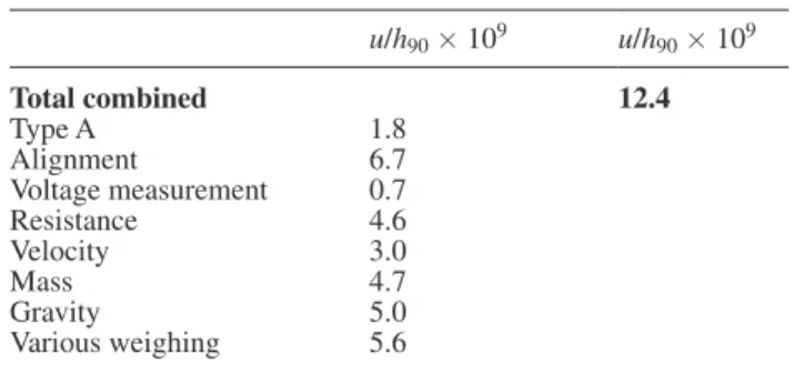
determination sorted into common categories. The uncertainties are in units of u/h90 × 10−9.

Uncertainty budget summary of the 6th determination

u/h90 × 109 u/h90 × 109 Total combined 12.4 Type A 1.8 Alignment 6.7 Voltage measurement 0.7 Resistance 4.6 Velocity 3.0 Mass 4.7 Gravity 5.0 Various weighing 5.6 Metrologia 54 (2017) 399

times of the pair of determinations. If the product of those varia-tions is constant (or nearly constant) then the correlation is ‘1’. If the product of those variations vary randomly, or even systemati-cally, over most of the uncertainty estimate then the correlation is ‘0’. It is the varying or randomization of the effect over the times of the two determinations that sets the value of the correlation.

Table A2 shows the 6th uncertainty budget sorted into common categories. It is interesting to note that the comp-onents of alignment, resistance, mass and gravity are all com-parable in magnitude. Any future improvements will require advances in all four areas. Table A3 shows the correlation of each of the seven Planck determinations with each other.

Appendix B. Covariant analysis

We have seven determinations of a variable y, each with an uncertainty budget consisting of 58 uncertainty components, as well as correlation assessments between all possible uncer-tainty components.

For the kth uncertainty component the vector, Sk, is made of the seven uncertainties,  uk i,, associated with kth component

  [ ]

=

Sk uk,1,uk,2,uk,3,uk,4,uk,5,uk,6,uk,7

(B.1) Similarly, the cross-correlations of the uncertainties of the kth component, between the ith determination and the other seven determinations is CCk i,  which is a seven element row vector made of 1 s and 0 s. See table A1.

The 7 × 7 correlation sub-matrix, CCk, of the kth uncer-tainty component is given by seven cross-correlation vectors, CCk,i of that component,

⎡ ⎣ ⎢ ⎢ ⎢ ⎢ ⎢ ⎢ ⎢ ⎢ ⎤ ⎦ ⎥ ⎥ ⎥ ⎥ ⎥ ⎥ ⎥ ⎥ = CC CC CC CC CC CC CC CC k k k k k k k k ,1 ,2 ,3 ,4 ,5 ,6 ,7 (B.2)

And the kth covariance sub-matrix, Ck is given by,

( ) =

Ck SkCCkSkT

(B.3) The total covariance matrix, C is then given by the sum of the 58 covariance sub-matrices.

To solve for the best estimate of an inverse covariance weighted mean, y, we create the row vector

= − − − − − − −

Y [ y₁ y,  y₂ y,  y₃ y,  y₄ y,  y₅ y,  y₆ y, y₇ y] (B.4) and note that the chi-squared is given by

(  )

χ2= YC Y−1 T

(B.5) Solving for y is obtained by minimizing chi squared with respect to y. The solution is a consequence of the Gauss Markov theorem which states that in a linear regression model in which the errors have expectation zero and are uncorrelated

and have equal variances, the best linear unbiased estimator (BLUE) of the coeficients is given by the ordinary least squares estimator. The technique of minimizing the chi-squared is very general and also used by the CODATA TGFC primarily because it is more robust for non-linear solutions.

[ ] = U If 1, 1, 1, 1, 1, 1, 1 (B.6) ( ) σ _{= UC U}− −

then the variance of the weighted mean is given by

y T 2 1 1 (B.7) χ = − n

and the Birge ratio is given by BR

1 2

(B.8)

References

[1] 2014 Resolution 1 of the 25th CGPM www.bipm.org/en/ CGPM/db/25/1/

[2] CCU/CCM SI Roadmap www.bipm.org/en/ measurement-units/rev-si/

[3] NIST Reference on Constants http://physics.nist.gov/cuu/ Constants/index.html

[4] SI brochure 9th edition www.bipm.org/en/measurement-units/ rev-si/#communication

[5] Sanchez C A, Wood B M, Green R G, Liard J O and Inglis D 2014 A determination of Planck’s constant using the NRC watt balance Metrologia 51 S5_–14

[6] Sanchez C A, Wood B M, Green R G, Liard J O and Inglis D 2015 Corrigendum to the 2014 NRC determination of Planck’s constant Metrologia 52 L23

[7] Sanchez C A, Wood B M, Inglis D and Robinson I A 2013 Elimination of mass exchange errors in the NRC watt balance IEEE Trans. Instrum. Meas. 62 1506_–11

[8] Sanchez C A and Wood B M 2014 Alignment of the NRC watt balance: considerations uncertainties and techniques Metrologia 51 S42_–53

[9] CCU 22nd meeting www.bipm.org/en/committees/cc/ccu/ publications-cc.html

[10] Robinson I A 2012 Towards the redeinition of the kilogram: a measurement of the Planck constant using the NPL Mark II watt balance Metrologia 49 113_–56

[11] Haddad D, Seifert F, Chao L S, Li S, Newell D B, Pratt J R, Williams C and Schlamminger S 2016 A precise instrument to determine the Planck constant and the future kilogram Rev. Sci. Inst. 87 061301

[12] Schwarz J P, Liu R, Newell D B, Steiner R L, Williams E R, Smith D, Erdemir A and Woodford J 2001 Hysteresis and related error mechanisms in the NIST watt balance experiment J. Res. Natl Inst. Stand. Technol. 106 627_–40

[13] Li S, Zhang Z and Han B 2013 Nonlinear magnetic error evaluation of a two-mode watt balance experiment Metrologia 50 482_–9

[14] Liard J O, Sanchez C A, Wood B M, Inglis A D and Silliker R J 2014 Gravimetry for watt balance measurements Metrologia 51 S32_–41

[15] Davidson S 2010 Determination of the effect of transfer between vacuum and air on mass standards of platinum– iridium and stainless steel Metrologia 47 487_–97

[16] Davidson S, Berry J, Abbott P, Marti K, Green R, Malengo A and Nielsen L 2016 Air-vacuum transfer; establishing traceability to the new kilogram Metrologia 53 A95–113

[17] Mohr P J, Newell D B and Taylor B N 2016 CODATA recommended values of the fundamental physical constants: 2014 Rev. Mod. Phys. 88 035009