Deep neural networks for audio scene recognition

HAL Id: hal-01888746

https://hal.archives-ouvertes.fr/hal-01888746

Submitted on 26 Mar 2020

HAL is a multi-disciplinary open access

archive for the deposit and dissemination of

sci-entific research documents, whether they are

pub-lished or not. The documents may come from

teaching and research institutions in France or

abroad, or from public or private research centers.

L’archive ouverte pluridisciplinaire HAL, est

destinée au dépôt et à la diffusion de documents

scientifiques de niveau recherche, publiés ou non,

émanant des établissements d’enseignement et de

recherche français ou étrangers, des laboratoires

publics ou privés.

Deep neural networks for audio scene recognition

Yohan Petetin, Cyrille Laroche, Aurelien Mayoue

To cite this version:

Yohan Petetin, Cyrille Laroche, Aurelien Mayoue. Deep neural networks for audio scene recognition.

2015 23rd European Signal Processing Conference (EUSIPCO), Aug 2015, Nice, France. pp.7362358,

�10.1109/EUSIPCO.2015.7362358�. �hal-01888746�

DEEP NEURAL NETWORKS FOR AUDIO SCENE RECOGNITION

Yohan Petetin, Cyrille Laroche, Aur´elien Mayoue

CEA, LIST, Gif-sur-Yvette, F-91191, France

ABSTRACT

These last years, artificial neural networks (ANN) have known a renewed interest since efficient training procedures have emerged to learn the so called deep neural networks (DNN), i.e. ANN with at least two hidden layers. In the same time, the computational auditory scene recognition (CASR) problem which consists in estimating the environment around a device from the received audio signal has been investigated. Most of works which deal with the CASR problem have tried to find well-adapted features for this problem. However, these features are generally combined with a classical classi-fier. In this paper, we introduce DNN in the CASR field and we show that such networks can provide promising results and perform better than standard classifiers when the same features are used.

Index Terms— Deep neural networks; deep beliefs

net-works; audio scene recognition.

1. INTRODUCTION 1.1. Generalities

The CASR problem consists in determining automatically the context or environment around a device [1]. A variety of features have been proposed for CASR, but the majority of the past work uses features that are well-known for struc-tured data, such as speech and music. In this way, time-domain (zero-crossing rate), frequency-time-domain (band-energy ration, spectral centroid, spectral flatness) and cepstral (Mel-frequency cepstral coefficients) features are naturally used in the literature [1] [2] [3] [4]. Only few recent articles have pro-posed new sets of features which try to encode some relevant information for unstructured environmental sound classifica-tion. The choice of these new features is often inspired by other research fields than audio one such as image process-ing (spectrogram pattern [5], histogram of gradient (HOG) features [6]), chaos theory (Recurrence Quantification Analy-sis descriptors [7]) or compressed sensing (Matching Pursuit-based features [8]). In this paper, we do not discuss on the relevance of audio features for CASR but we investigate clas-sification approaches. Indeed, whatever the complexity of the features proposed in the literature, the classification step is always based on standard machine learning approaches such as K-nearest neighbors [1] [5] [8], Gaussian Mixture

Mod-els (GMM) [1] [8], hidden Markov modMod-els [2] [3], Support Vector Machines (SVM) [4] [6] [7]. Or, while DNN have led to significant advances in automatic speech recognition [9], this approach has never been used in the field of CASR to the best of our knowledge. In this paper, we study how to deploy DNN for audio context recognition and we show that DNN can produce promising results even when we use stan-dard audio features which are not necessarily optimized for the CASR problem.

1.2. Feed forward artificial neural networks

Feed forward artifical neural networks (ANN) are popular computer architectures which can be used for classification. More precisely, when the objective is to classify a feature of interest x among C classes, an ANN estimates the probabili-ties pj, j ∈ {1, · · · , C}, of each class given the input feature

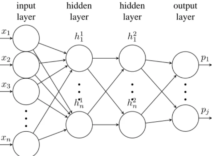
x. In our audio classification problem, the input x represents the concatenation of audio features [10] [11], such as cepstral (Mel-frequency cepstral coefficients (MFCC)) and frequency features (spectral centroid, spectral flatness,...); the class rep-resents the audio context (car, bus, office, street, restaurant, ...). A graphical representation of this architecture is given in Figure 1.

..

.

..

.

..

.

..

.

Fig. 1. An ANN is described by an input (a feature vector), a given number of hidden layers, a given number of neurons per layer and an output which describes the class probabilities.

need to compute the ouput of each hidden unit. In an ANN, the connection between the k− 1-th hidden layer and the k-th one is described by a matrix of weights Wk, and a bias vector bk_{; the output h}k

j of the j-th neuron of the k-th layer is then

computed from hkj = f X i wijkh k−1 i + b k j ! , (1)

where f(.) is the sigmoid function: f(x) = sigmoid(x) = 1

1 + e−x. (2)

Finally, the output is computed via the softmax nonlinearity, pj = ePi=1w p ijh p−1 i +b p j P ke P i=1w p ikh p−1 i +b p k , (3)

where p is the number of layers (without counting up the input layer).

The training of ANN (i.e. the estimation of parameters Wkand bk) relies on supervised methods such as the Back-Propagation (BP) algorithm [12] whose the principle will be reminded in section 3. However, when the number of hid-den layers and neurons increases, supervised methods are not reliable and ANN are difficult to tune. Particularly, these methods can be stuck in a poor local optima when we look for estimating the parameters. Recently, new procedures for training DNN (i.e. ANN with at least two hidden layers) have been proposed to overcome the limitations of classi-cal training algorithms [13] and rely on an unsupervised pre-training which aims at initializing properly the parameters of the DNN. The rest of this paper is organized as follows. In Section 2, we describe the pre-training step of DNN which relies on Restricted Boltzman Machines (RBM) and Deep Be-lief Networks (DBN) and which are both probabilistic graphi-cal models. In Section 3, the principle of the supervised train-ing via the BP algorithm is recalled. Finally, in section 4, we focus on the tuning of DNN for CASR problem by perform-ing experimentations on an audio context dataset.

2. PRE-TRAINING OF DNN VIA DBN

We now focus on the initialization of the parameters of DNN by considering DBN which are generative graphical model. Thus, the initialization of the parameter of a DNN relies on those of the associated DBN. However, maximizing the likeli-hood of a DBN is impossible. Consequently variational meth-ods based on RBM models have been developed and con-sists in training separately each layer of the DBN as an RBM. These models are described in our next paragraph.

2.1. RBM

An RBM is a probabilistic graphical model which connects a set of m visible random variables (r.v.), v = (v1,· · · , vm),

with a set of q hidden r.v., h = (h1,· · · , hq) [14]. In this

model, the joint probability density function (pdf) of the visi-ble and hidden units depends on an energy function and reads

p(v, h) = 1 Ze −E(v,h)_{, (4)} where E(v, h) = −X i aivi− X j bjhj− X i,j wijvihj, (5) Z =X v,h e−E(v,h) (6)

for a Bernoulli-Bernoulli RBM (BBRBM) (i.e. an RBM in which viand hjtake their values in{0, 1}). Equations related

to a Gaussian-Bernoulli RBM (GBRBM) and which are more adapted for real values can be found in [9].

From an unlabeled visible dataset(x1_{,· · · , x}N_{), our}

ob-jective is to learn the parameters of the RBM. More precisely, starting from (4)-(6), we intend to maximize the likelihood p(x1_{,· · · , x}N_{) =}QN i=1p(xi), where p(xi_{) =}X h p(xi_{, h) =} 1 Z X h e−E(xi,h), (7) w.r.t. ai, bjand wij.

However, the gradient of the log-likelihood, 1 N N X k=1 ∂log p(xk₎ ∂wij = 1 N N X k=1 X hj p(hj|xk)xkihj− X vi,hj vihjp(vi, hj), (8)

is not computable but can be interpreted as the sum of two expectations. Consequently, (8) can be approximated by a Monte Carlo method. More precisely, in an RBM (4), one can show that

p(hj = 1|v) = sigmoid(bj+

X

i

wijvi), (9)

where the sigmoid functionsigmoid(.) is defined in (2) and that

p(vi= 1|h) = sigmoid(ai+

X

j

wijhj). (10)

Finally, the first expectation in (8) is easy to approxi-mate by sampling according to p(vi|h); sampling

accord-ing to p(vi, hj) is more difficult but can be achieved via

a Gibbs sampler in which we sample alternatively from p(v|h) = Qm

i=1p(vi|h) and p(h|v) = Q q

i=jp(hj|v). In

practice, the expectations are approximated with only 1 sample and the Gibbs sampler relies on 1 iteration. This procedure is called the Contrastive Divergence (CD-1) algo-rithm and leads to an approximate maximization of (8) via a gradient descent method.

2.2. Deep Belief Networks

Let us now consider the DBN probabilistic model defined by a layer of visible unit x = h0 _{(our input data) and}

p− 1 hidden layers, denoted h1_{,· · · , h}p−1_{. The pdf of}

(h0, h1,· · · , hp−1) in a DBN reads p(h0, h1,· · · , hp) = p−2 Y i=1 p(hi−1|hi)p(hp−2, hp−1), (11) where p(hp−2_{, h}p−1_{) is an RBM and coincides with (4), and}

p(hi−1_|hi_{) is deduced from (10).}

Again, the maximization of the likelihood p(x) in model (11) w.r.t parameters Wkand bk associated to each layer hk is not possible. A greedy layer wise procedure has been pro-posed in the literature [13] [15] [16] and consists in approxi-mating the DBN (11) as a stacking of RBM (4).

Strictly speaking, p(hk−1_{, h}k_{) in (11) does not satisfy (4)}

and so is not an RBM, except for k= p − 1. However, justi-fications of the following procedure can be found in [16] [13] and relies on Kullback Leibler Divergence arguments.

In summary, the unsupervised training of a DBN (i.e. the pre-training of our DNN) consists of the following steps; starting from a training dataset{x1_{,· · · , x}i_{,· · · , x}N_{} :}

1. train the first RBM (h0_{, h}1_{) (i.e. compute W}1 _{and b}1

associated to the first layer) via the procedure described in section 2.1;

2. compute the output associated to the data set{x1_{,· · · , x}i_,

· · · , xN_{} via (1)-(2) using the parameters W}1_{and b}1

ob-tained after the pre-training;

3. train the next RBM (h1_{, h}2_{), · · · , (h}p−2_{, h}p−1_{) by}

re-peating steps 1. and 2.

3. FINE-TRAINING OF DNN

We now consider that the parameters estimated by the pre-training algorithm are used for the initialization of the super-vised training algorithm of the DNN. So now we assume that we have a set of labeled data

E= {(x1, d1), · · · , (xi_{, d}i_{), · · · , (x}N_{, d}N_{)} (12)}

where di _{= [d}i

1,· · · , diK]T is the known class vector

asso-ciated to xi _{and K the number of classes: d}i

j=C = 1 if xi

belongs to the C-th class and di

j6=C= 0 otherwise. Note that

this set could be different from the one used in the previous section for the learning of the associated DBN.

Supervised training consists in tuning matrices Wk and biases bkfrom the set E in (12). Here, our objective is to min-imize the cross entropy C= −PK

k=1dklog(pk) between the

output of the DNN p = [p1,· · · , pK]T and the target

prob-abilities d = [d1,· · · , dK]T. The BP method is a popular

algorithm to compute recursively the gradient of C w.r.t. the weights wk

ij and the biases bkj of the DNN [12]. Finally, the

algorithm includes a gradient descent method in order to ap-proximate the parameters which minimize C.

In summary, from a given labeled data (x, d) and for a given iteration l:

1. Compute the output p associated to the input x by using weights wk

ij(l − 1) and biases bkj(l − 1) of the previous

iteration l− 1. Remember that wk

ij(0) and bkj(0) coincide

with the parameters estimated by the pre-training step; 2. Backpropagate the gradient of the error C in the DNN, i.e.

compute the gradient∆wk

ij(l) and ∆bkj(l) of C w.r.t the

weights and the biases of the DNN. 3. Update the weights wk_ij(l) = wk

ij(l − 1) − ǫ∆w k ij(l), and the biases bk_j(l) = bk j(l − 1) − ǫ∆b k j(l), where ǫ is the learning rate;

Many refinements have been proposed in order to improve the computation of the weights and the biases from the train-ing set E in (12). These refinements rely on a random mini-batch to compute the gradient of the error and the momentum method to improve the speed of learning [17].

4. SIMULATIONS 4.1. Dataset

We present the results for audio context classification that we have obtained with DNN. The dataset that we use in this section is the publicly available audio scene dataset acquired by the LITIS Rouen [18]. The dataset is composed of3026 recordings whose duration is30 seconds in such a way that about1500 minutes of audio scene have been recorded. The data are scattered in 19 classes : plane, bus, busy street, cafe, car, student hall, train station hall, kid game hall, mar-ket, metro-paris, metro-rouen, billard pool hall, quiet street, restaurant, pedestrian street, shop, train, high-speed train and tubestation. More details on the dataset can be found in [6].

Our experimentations are based on a standard feature set which consists in computing12 MFCC, its first order deriva-tives (∆MFCC) and 6 subband spectral flatness coefficients [19] for every15ms-spaced frames of length 30ms.

To evaluate our system, we have followed the protocol proposed in [6] i.e.80% of the examples were used for train-ing while the remaintrain-ing recordtrain-ings were kept for testtrain-ing (and results were averaged over20 different splits of the dataset). As an evaluation criterion, we have considered the recogni-tion rate. Since the classes are not represented by the same number of recordings, the recognition rate reads

Rec Rate = 1 C C X i=1 TP(i) Card(C(i)),

where C = 19, TP(i) is the number of examples of class i correctly classified andCard(C(i)) the number of examples in class i. The final decision for a recording is taken by first

averaging the output of the DNN for each input frame which forms the recording and next choosing the class with the best result.

On one hand, our simulations aim at studying the perfor-mances of DNN for CASR in function of the number of hid-den layers and the number of neurons for a given layer. On the other hand, we also study the effect of the number of the concatened frames of30ms (1, 5, 10...) at the input of the DNN.

Finally, to be sure that our experiments are reproducible by others, we mention the specific parameters we have used for the learning procedures. The number of epochs for the pre-training and the fine-training is100 and 300 respectively; the learning set is set to1 for the pre-training and 0.1 for the supervised training; a batch size of100 is used for both train-ing procedure; the momentum is set to0.5 for the first five epochs of both training and next to0.9. Finally, a weight cost is set to0.2 × 10−5, for the pre-training. An interpretation of these parameters can be found in [17].

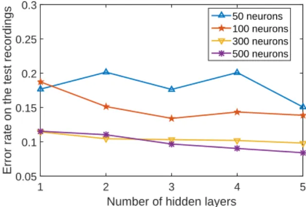
4.1.1. Influence of the size of the DNN

In this paragraph, we consider a fixed number of 15 input frames (so the size of the input layer of our DNN is15× 30 = 450) and we compare the performances in function of the number of hidden layers and the number of neurons for each hidden layer. For simplicity, we have considered the same number of neurons for each hidden layer. In figure 2 we have displayed the recognition rate in function of these parameters. Overall, DNN perform better when the number of hidden lay-ers and neurons is greater but it can be seen that when the number of neurons is weak, increasing the number of hidden layers does not necessarily improve the performances. The worse recognition rate (80%) is obtained for 2 hidden layers of50 neurons and the best performances (91.6%) are obtained with5 hidden layers of 500 neurons. For reasons of space, we have not reproduced the confusion matrix associated to this configuration. Roughly speaking, all classes have a recog-nition rate greater than80%, except the quiet street and the pedestrian street which have a recognition rate of66.66% and 75%, respectively. Theses classes are mainly confused with the shop and market classes. For larger DNN, we have not ob-served a major improvement. Indeed, for a DNN with7 hid-den layers and1000 neurons, the recognition rate is 92.2%.

4.1.2. Influence of the input of the DNN

We now set the number of hidden layers to3 and the num-ber of neurons to50 and we perform a simulation in function of the number of input frames. Increasing the number of in-put frames has the advantage to reduce the comin-putational cost when we need to do many classifications. From a computa-tional cost point of view, it is clear that it is preferable to use 30 × 15 = 450 coefficients at the input of the DNN rather

Number of hidden layers

1 2 3 4 5

Error rate on the test recordings_0.05

0.1 0.15 0.2 0.25 0.3 50 neurons 100 neurons 300 neurons 500 neurons

Fig. 2. Performances of DNNs for audio classification scene in function of the size of the DNN. Here, the number of input frames is15.

Number of concatenated frames in input

0 10 20 30 40 50

Error rate for recordings

0.16 0.18 0.2 0.22 0.24 0.26 0.28 0.3 Error rate

Fig. 3. Error rate in terms of recordings for the validation set in function of the number of input frames. The DNN has3 hidden layers of50 neurons.

than doing15 classifications with 30 coefficients. However, when the final decision is taken after several classifications, the mean error rate per recording is optimal for10-15 frames as we see in Fig. 3.

We have also computed a classifier based on Gaussian Mixture models (GMM). We have trained4 mixtures for each class via the Expectation Maximization (EM) algorithm. The best recognition rate for this classification method is80.91% and is obtained by considering one input frame. It seems that the concatenation of frames is only interesting for architec-tures like DNN because they permit to encode the temporal connections between the frames. This observation is also con-firmed by the fact that DNN present similar results if we do not consider the∆MFCC which describe such connections. Finally, we have also computed a SVM classifier with a Gaus-sian Kernel and15 concatenated input frames. The recogni-tion rate is 86.5 %.

5. CONCLUSION

We have proposed a DNN-based approach for the CASR problem. The rationale of the training algorithms associated to DNN has been recalled and the performances of these architectures have been studied in function of their size and of the number of concatenated input frames, which define the input layer of the DNN. DNN have been compared with more classical classifiers such as GMM and SVM, with the same features: the optimal recognition rates obtained are 92%, 81% and 86.5%, respectively. The relevance of the features used in our simulations have not been discussed, but we underline that DNN applied to standard features give sim-ilar results as well-defined features (HOG) classified by an SVM approach [6] following the same protocol on the same dataset (best performance is92% in both cases). In this way, several solutions could be exploited in order to improve the performances of DNN in this context. First, more adapted features (HOG features for example) could be used at the input of the DNN. Alternatively, we could also let the DNN extract automatically the relevant features by using directly the spectrum as input.

REFERENCES

[1] V. T. Peltonen, J. T. Tuomi, A. Klapuri, J. Huopaniemi, and T. Sorsa, “Computational auditory scene recog-nition,” in International Conference on Acoustics, Speech, and Signal Processing (ICASSP), 2002, pp. 1941–1944.

[2] A. Eronen, V. Peltonen, V. Tuomi, A. Klapuri, S. Fager-lund, T. Sorsa, G. Lorho, and J. Huopaniemi, “Audio-based context recognition,” IEEE Transactions on Au-dio, Speech and Language Processing, vol. 14, pp. 321– 329, 2006.

[3] L. Ma, B. Milner, and D. Smith, “Acoustic environ-ment classification,” ACM Transactions on Speech and Language Processing, pp. 1–22, 2006.

[4] M. Perttunen, M. Van Kleek, O. Lassila, and Riekki J., “Auditory context recognition using SVMs,” in Mobile Ubiquitous Computing, Systems, Services and Technologies (UBICOMM08),Valencia, Spain, 2008, pp. 102–108.

[5] P. Khunarsal, C. Lursinsap, and T. Raicharoen, “Very short time environmental sound classification based on spectrogram pattern matching,” Information Sciences, vol. 243, pp. 57–74, 2013.

[6] A. Rakotomamonjy and G. Gasso, “Histogram of gradi-ents of time-frequency representations for audio scene classification,” IEEE Transactions on Audio, Speech and Language Processing, vol. 23, no. 1, pp. 142–153, 2015.

[7] G. Roma, W. Nogueira, and P. Herrera, “Recur-rence quantification analysis features for environmental sound recognition,” in IEEE AASP Challenge on Detec-tion and ClassificaDetec-tion of Acoustic Scenes and Events, 2013, pp. 1–4.

[8] S. Chu, S. Narayanan, and C.-C. J. Kuo, “Environmen-tal sound recognition with time-frequency audio fea-tures,” IEEE Transactions on Audio, Speech and Lan-gage Processing, vol. 17, no. 6, pp. 1142–1158, 2009. [9] G. E. Hinton, L. Deng, D. Yu, G. E. Dahl, Mohamed

A-R., N. Jaitly, A. Senior, V. Vanhoucke, P. Nguyen, T.N Sainath, and B. Kingsbury, “Deep neural networks for acoustic modeling in speech recognition: The shared views of four research groups,” IEEE Signal Procesing. Magazine, vol. 29, no. 6, pp. 82–97, 2012.

[10] A. Mohamed, G. E. Dahl, and G. Hinton, “Acoustic modeling using deep belief networks,” IEEE Transac-tions on Audio, Speech and Langage Processing, vol. 20, no. 1, pp. 14–22, Jan. 2012.

[11] H. A. Bourlard and N. Morgan, Connectionist Speech Recognition: A Hybrid Approach, Kluwer Academic Publishers, Norwell, MA, USA, 1993.

[12] D. E. Rumelhart, G. E. Hinton, and R. J. Williams, “Neurocomputing: Foundations of research,” chapter Learning Representations by Back-propagating Errors, pp. 696–699. MIT Press, Cambridge, MA, USA, 1988. [13] G. E. Hinton, S. Osindero, and Y-W. Teh, “A fast learn-ing algorithm for deep belief nets,” Neural Computa-tion, vol. 18, no. 7, pp. 1527–1554, July 2006.

[14] H. Larochelle and Y. Bengio, “Classification using dis-criminative restricted boltzmann machines,” in Pro-ceedings of the 25th International Conference on Ma-chine Learning, 2008, pp. 536–543.

[15] C. Poultney, S. Chopra, and Y. Lecun, “Efficient learning of sparse representations with an energy-based model,” in Advances in Neural Information Processing Systems (NIPS) 2006. 2006, MIT Press.

[16] B. Yoshua, Learning Deep Architectures for AI, Now Publishers Inc., 2009.

[17] G. E. Hinton, “A practical guide to training restricted Boltzmann machines.,” in Neural Networks: Tricks of the Trade (2nd ed.), Grgoire Montavon, Genevieve B. Orr, and Klaus-Robert Mller, Eds., vol. 7700 of Lecture Notes in Computer Science, pp. 599–619. 2012. [18] “LITIS Rouen audio dataset,” https://sites.google.com

/site/alainrakotomamonjy/home/audio-scene.

[19] A. Ramalingam and S. Krishnan, “Gaussian mixture modeling of short-time Fourier transform features for audio fingerprinting,” IEEE Trans. Info. For. Sec., vol. 1, no. 4, pp. 457–463, 2006.