Analysis of Gene Evolution: the software AGE

CABIOS

Analysis of Gene Evolution: the software AGE

Didier G. Arques, Christian J.Michel1'3 and Karine Orieux2

Abstract

The software AGE (Analysis of Gene Evolution) has been developed both to study a genetic reality, i. e. the identification of statistical properties in genes (e.g. periodicities), and to simulate this observed genetic reality, by models of molecular evolution. AGE has two types of models: CO models of sequence creation from oligonucleotides: concatenation model in series of an oligonucleotide, independent (or Markov) mixing model of oligonucleotides according to given probabilities (or a Markov matrix); (ii) models of sequence evolution from created sequences: insertion/deletion process of (mono,di,tri)nucleot-ides, base mutation process. The study of a reality and the development of simulation models are based on several new algorithms: approximated simulation and exact calculus to compute various autocorrelation functions, Fourier transforma-tion of autocorrelatransforma-tion curves, recognitransforma-tion of a curve form, etc. AGE is implemented on IBM or compatible microcomputers and can be used by biologists without any computer knowledge to identify statistical properties in their newly determined DNA sequence and to explain them by models of molecular evolution.

Introduction

Context

The determination of nucleotides, their storage in gene databases and their analysis via mathematics, statistics and computer science, have allowed the development of theories of molecular evolution of genes (e.g. Eigen and Schuster, 1978; Kimura, 1987). In particular, the recent development of computer sciences, i.e. in terms of algorithms, calculus power and data structures, represents at the moment the only way to analyse several millions of nucleotides. In this context, we have recently developed a new model of DNA sequence evolution showing that the actual genes may derive from a mixing of only a few types of primitive oligonucleotides (Arques and Michel, 1990b).

Univerziti de Franche-Comi, Laboraloire d'Informatique de Besancon, Uniti Associte CNRS No. 822, 16 route de Cray, F-25030 Besancon, France, 'Friedrich Miescher Institut, Bioinjbrmatic Croup, Mattenslrasse 22, PO Box 2543, CH-4002 Basel, Switzerland and 2Universiti de Haute-Alsace,

Laboraloire de MathimaAque el lnformatique, Faculti des Sciences el Techniques, 4-rue des Frires Lumiere, F-68093 Mulhouse, France

3Presenl address: Equipe de Biohgie Theorique, Universili de Franche-Comi,

Institut Universilaire de Technologie de Belfort-Montbiltard, BP 527, 90016 Belfort, France.

The algorithms associated with this model have been gathered and generalized in a software package implemented on IBM or compatible microcomputers, and called AGE (Analysis of Gene Evolution). We also give here the algorithm of exact calculus of an autocorrelation function in its general form; a particular case of this new algorithm was used, but not described, in Arques and Michel (1990b, p. 756).

In order to understand the functionalities of AGE, we briefly recall the approach that forms the basis of this new model (described in detail in Arques and Michel, 1990b). The approach consists of two successive steps: firstly, the study of a genetic reality, i.e. the identification of statistical properties in genes (e.g. periodicities, maximal and minimal values, etc); and secondly, the simulation of this observed genetic reality. Indeed, as the combination of nucleotides is high, a simulation model, i.e. a model correlated with the reality, can only be found after an initial study of a genetic reality. We also have shown that such simulation models exist by using primitive oligonucleot-ides. Thus, these simulation models are molecular evolution models. Finally, we have identified a particular class of functions, called autocorrelation functions, allowing both the identification of statistical properties in genes and the develop-ment of molecular evolution models in order to simulate them. An autocorrelation function gives the occurrence frequency of a motif (series of nucleotides) / bases after another motif (eventually the same) in a gene population (or in one gene). A definition, for a particular case, is given in the algorithm section.

Study of a genetic reality

The phylogenetic tree of genes, commonly accepted to be overall divergent, shows two aspects, (i) The diversity or the specificity with the actual genes (i.e. the leafs of the phylogenetic tree), which can be studied by applying a function at the gene level, (ii) The common base in a few primitive genes (i.e. the root of the phylogenetic tree). In Arques and Michel (1990b), we were interested in the common properties in genes (i.e. common in all leaves of the phylogenetic tree, and therefore deriving from its root) and we have shown that they can be identified by applying an autocorrelation function at the gene population level (i.e. a set of several hundreds of genes allows the application of the law of large numbers; see Arques and Michel, 1990b, p. 752, section 2.3.3 for the details). More precisely, by applying the autocorrelation function using the

trinucleotide YRY (see section 'Autocorrelation function YRY') in —20 gene populations, three statistical properties common in genes have been identified: the YRY(N)6YRY preferential occurrence (R = purine = A or G, Y = pyrimidine = C or T, N = R or Y; Arques and Michel, 1987b, 1990a), the periodicity modulo 3 (P3) (Fickett, 1982; Arques and Michel, 1987a, 1990a) and the periodicity modulo 2 (P2) (Arques and Michel, 1987c, 1990a).

Simulation of this observed genetic reality

In Arques and Michel (1990b) we proved that these three common statistical properties, and also features specific to a subset of gene populations, can be surprisingly retrieved with a unique simulation model based on the independent (not Markov) mixing of the three primitive oligonucleotides

YRYYRY, YRYRYR and YRY(N)6, i.e. based on a random

mixing only depending on the proportion of these three oligonucleotides. On the other hand, these three common statistical properties can also be simulated with a similar (reasons not given here) model that randomly inserts and deletes (mono,di,tri)nucleotides (a process similar to the one called in biology 'RNA editing') in sequences composed of a primitive oligonucleotide concatenated in series (Arques and Michel,

1991).

Aims of the software AGE

AGE can study a genetic reality by computing any autocorrela-tion funcautocorrela-tion in the alphabet (R,Y) (i.e. not only related to the trinucleotide YRY) in a gene population or in a sequence. The associated curve is called the real curve. This functionality should allow the identification of new statistical properties in genes: common statistical properties by applying autocorrela-tion funcautocorrela-tions in gene populaautocorrela-tions, and specific statistical properties by applying autocorrelation functions in a sequence already known or newly determined.

AGE has two types of molecular evolution models. Models of sequence creation. The sequences are created from primitive oligonucleotides: concatenation model in series of a primitive oligonucleotide, e.g. the sequence (YRY(N)3)* = YRY(N)3YRY(N)3 . . . is created by the concatenation in series of the primitive oligonucleotide YRY(N>3; independent (or Markov) mixing model of primitive oligonucleotides (up to 10) according to given probabilities (or a Markov matrix)— this option allows the creation of complex sequences. Models of sequence evolution. The sequences created can be subjected to an evolutionary process in steps: process of random insertions and/or deletions of (mono,di,tri)nucleotides; process of base mutation by random transformation of bases, R (respectively Y) giving Y (respectively R).

AGE analyses all of these models by computing any auto-correlation function on the alphabet (R,Y) for any model. The associated curve is called the simulated curve. A model

simulates (i.e. is correlated with) the reality if its associated simulated curve has the same statistical properties compared to the real curve by applying the same autocorrelation function. These two functionalities should allow the identification of other primitive oligonucleotides, the study of gene dating, base mutations, etc. Furthermore, the simulation models also reveal properties hidden in the reality (return of the model to the

reality; see Arques and Michel, 1990b, p. 766).

Computer analysis work for the develoment of the software AGE

The computer analysis work for the development of AGE has mainly dealt with four points.

(i) Definition of the functionalities (see previous section). In order to facilitate the use of AGE as a research tool, additional functionalities have been included such as Fourier transforma-tion of an autocorrelatransforma-tion curve, algorithm of curve form recognition, etc.

(ii) Definition of data structures, in particular those related to the files: storage of autocorrelation curves in order to avoid new computations, direct access of an autocorrelation curve to get a fast visualization, storage of A, C, G and T of DNA sequences in 2 bits to compress the files, etc. (see section 'Data structures' below).

(iii) Resolution of problems of complexity. Scanning by varying the proportion of primitive oligonucleotides in an independent (or Markov) mixing model leads to the analysis of several thousands of possible situations. A calculus of complexity shows that such a scanning cannot be realized by an algorithm that generates a population of simulated sequences for each situation, but can be done by an algorithm of exact calculus (see section 'Problem of complexity' below).

(iv) An interactive and user-friendly software that can be used without any computer knowledge. Several utilities have been developed concerning the entry and modification of data by menus, automatic manipulation of files, graphic tools, etc. (see section 'Utilities available' below).

System and methods

AGE is implemented on IBM or compatible microcomputer with a standard graphics VGA video card. The source code contains —8500 Pascal lines in 13 units, each unit corresponding to a functionality. This structure in units easily allows modifications and extensions of AGE. The executable file needs 170 kbytes. The output of AGE, in particular the figures, includes PostScript, thereby allowing the use of a broad range of printing devices.

Algorithm

Autocorrelation function YRY

Let F be a gene population with n(F) sequences. Let j b e a

Analysis of Gene Evolution

YRY(N),YRY (R = purine = A or G, Y = pyrimidine = C or T, N = R or Y) by varying / in the range [0,99], be two trinucleotides YRY separated by any / bases N. For each 5 of F, the counter cfe) counts the occurrences of m, in s. In order to count the m, occurrences in the same conditions for all i, only the first l(s) - 104 (= l(s) - (99 + 6) + 1) bases of s are examined (99 + 6 is the maximal length of m,). Then, the occurrence probability o,{s) of ny for s is equal to c,{s)/[l(s)

— 104], i.e. the ratio of the counter by the total number of current bases read. Then, the occurrence probability pt(F) of mt for F is equal to [LieFo,{s)]/n(F). For each population F, the function, called 'autocorrelation function YRY', i — p{F) by varying /, is represented as a curve C(F). In order to have a sufficient number of rru# occurrences, the function is applied to sequences having a minimal length of 250 bases.

The curve C(F) is represented as follows, (i) The abscissa shows the number i of bases N (R or Y) between two trinucleotides YRY by varying i between 0 and 99. (ii) The ordinate shows the occurrence frequency of YRY 1 bases after itself in a gene population F (see e.g. Figure la and b). Description of the software AGE

Each functionality of AGE will be illustrated with an example deduced from our previous results found with the autocorrela-tion funcautocorrela-tion YRY. In the study of a genetic reality, this particular autocorrelation function was applied in gene populations.

Functionality to study a genetic reality. Example: AGE with the autocorrelation function YRY applied in the two gene populations, eukaryotic introns and the 5' eukaryotic regions, reveals a periodicity P2 (modulo 2) in the range [0,L] defined as follows: p,{F) > max(/>, _ ,(f), p-, + ,(F)) with i G [0,L] and i a 1[2] (1 = 1 + 2n), i-e. / = 1, 3, 5, etc. Precisely: (i) The eukaryotic introns IEUK (1790 sequences from the EMBL release 21; Figure la) has the periodicity P2 in the range [0,L = 49] and the highest value p/(IEUK) at 1 = 1.

(ii) The 5' eukaryotic regions N5EUK (2489 sequences from the EMBL release 21; Figure lb) has the periodicity P2 in the range [0,L = 23], the highest value p,<N5EUK) at 1 = 3 and four obvious sets of points that can be joined by regular curves: (a) / = 3, 9, 15, 21, 27 and 33; (b) / = 1, 5, 7, 11, 13, 17, 19, 23 and 25; (c) 1 = 6, 12, 18 and 24; and (d) 1 = 2, 4, 8, 10, 14 and 16. All these naturally appearing curves join modulo 6 periodic sets of i values.

The curves of these two populations IEUK and N5EUK have non-random features. It should be stressed that the curve associated with an autocorrelation function can be 'random' (see, for example, the curve of the gene CLCK given in Arques and Michel, 1990b, p. 755). Such a random curve cannot be simulated using primitive oligonucleotides. Therefore to analyse genes in terms of primitive oligonucleotides, it is important to choose, if possible, an autocorrelation function leading to a curve with non-random properties such as the following:

0 S l O I S 2 0 a 5 J 0 3 S « 0 « S 5 0 S 3 H ) 6 S 7 0 7 5 8 0 8 S 9 0 « l O O

0 S 1 5 M E J O 3 ! « 1 5 S O 5 5 H ) B 5 7 1 ) 7 i e O K 9 O 9 5 I M

Fig. 1. Study of a genetic reality by applying the autocorrelation function YRY in gene populations (see section 'Functionality to study a genetic reality'). The horizontal axis represents the number / of bases N in the i-motif YRY(N)jYRY, with 1 e [0,99]. The vertical axis represents the frequency p,<f) in the following populations F: (a) eukaryotic introns IEUK showing the periodicity P2 (modulo 2) in the range [OX «• 49] and the highest value at i «• 1; (b) 5' eukaryotic regions N5EUK showing the periodicity P2 (modulo 2) in the range [OX •• 2 3 ] , the highest value at / - 3 and the four subcurves modulo 6.

Existence of a periodicity: modulo 2, 3, etc. This periodicity can be obvious (e.g. in IEUK and N5EUK), but in some cases it must be identified with a statistical test such as a binomial test (Arques and Michel, 1990a). According to the current state of statistical analyses, the periodicity modulo 2 has been only found in eukaryotic introns and in the 5' and 3' regions of eukaryotes. It was attributed to regulatory functions of genes (Arques and Michel, 1987c, 1990a). The periodicity modulo 3 is found in protein-coding genes of any taxonomic group: eukaryotes, prokaryotes, viruses, chloro-plasts, mitochondria and plasmids. It is related to the coding function of genes. This periodicity modulo 3 is also observed in introns of viruses (optimization of functions of a genome of small size) and mitochondria (maturases) (see Arques and Michel, 1990a, for the details).

Beginning and end of a periodicity. Several situations have already been observed and simulated: a periodicity modulo 3 in the range [0,99], a periodicity modulo 2 in the range [OX] with L < 99 (e.g. in EEUK and N5EUK), a periodicity modulo 2 in the range [0,L] and a periodicity modulo 3 in

YHYYIW: ut ir1

1

Hiiii

Fig. 2 . Independent mixing model of the three oligonucleotides YRYYRY, YRYRYR and YRY(N)6; curves associated with the autocorrelation function YRY

(see section 'Functionality of sequence creation'). ( a - Q Scanning varying the proportions in |2%,14%,26%| for YRYYRY and in (57%,69%,8l %| for YRYRYR, the proportion of YRY(N)6 being the complement to 100%. The simulated curve (e) is similar to the real curve IEUK (Figure la); the simulated curve (f) is similar to the real curve N5EUK (Figure lb).

the range [L,99] (Arques and Michel, 1990a,b). For example, it was explained in Arques and Michel (1990b) that the gene populations with a periodicity modulo 2 in the range [0,L] with a large value for L have large alternating purine/pyrimidine stretches.

Presence of a maximal (respectively minimal) value significantly greater (respectively less) than the other values (see, for example, the methodologies developed in Arques and Michel, 1987a,b, to identify important values of i in an autocorrelation curve). For example, the maximal value at i = 6 with the autocorrelation function YRY obtained in most of the genes (hidden in IEUK and N5EUK) has been related to a primitive code of the DNA helix pitch generated by the primitive oligonucleotide YRY(N)6 (Arques and Michel, 1987b, 1990b).

Presence of subcurves (e.g. in N5EUK), etc.

AGE can compute any autocorrelation function on the alphabet (R,Y) (not only related to the trinucleotide YRY) in a gene population or in a sequence and stores its associated curve

(see also section 'Data structures' below). The definition of the particular autocorrelation function YRY in a gene population, was presented in section 'Autocorrelation function YRY' above. Its generalization to motifs different from YRY is obvious. The definition of the autocorrelation function in a gene is also trivial: it is the particular case of a population containing one gene (n(F) = 1). The implementation of the computation of an autocorrelation function is given in to complementary ways (see next section: 'Functionality of sequence creation').

Functionality of sequence creation. Example: it was proved in Arques and Michel (1990b) that the real curves of the 5' eukaryotic regions N5EUK and eukaryotic introns IEUK can be simulated by an independent mixing of the three primitive

oligonucleotides YRYYRY, YRYRYR and YRY(N)6. For

example, if AGE mixes these three oligonucleotides by varying the proportions in (2%,14%,26%) for YRYYRY, in

(57%,69%,81%) for YRYRYR, the proportion of YRY(N)6

being the complement to 100%, then six simulated curves (Figure 2) associated with the autocorrelation function YRY, are obtained with this scanning.

Analysis of Gene Evolution

The simulated curve 2(e) has the statistical properties of the real curve IEUK (Figure la): periodicity P2 in the range [OX = 41] and the highest value at i = 1.

The simulated curve 2(f) has the statistical properties of the real curve N5EUK (Figure lb): periodicity P2 in the range [0,L = 23], the highest value at i = 3 and the four subcurves modulo 6.

AGE can compute any autocorrelation function on the alphabet (R,Y) either for the concatenation model in series of a primitive oligonucleotide or for the independent (or Markov) mixing model of primitive oligonucleotides. Note that the concatenation model is the particular case of a mixing model with one primitive oligonucleotide. For reasons of complexity (see section 'Problem of complexity' below), AGE has two types of algorithms.

(i) Algorithm of approximated simulation. This algorithm generates a population of simulated sequences according to the following choices: the number and the type of oligonucleotides, their associated probabilities and the type of mixing-independent or Markov. Then, the autocorrelation function in the simulated population is computed in the same way as in the real gene population. The simulated population must have at least 200 simulated sequences of length 1000 in order to obtain a significant simulated curve.

(ii) Algorithm of exact calculus. This algorithm, detailed in section 'Algorithm of exact calculus of the autocorrelation function' below, computes an autocorrelation function by a unique travel in depth of the lexicographical tree representing all possible series of oligonucleotides on the alphabet of oligonucleotides chosen. It avoids the effective generation in memory of a population of simulated sequences, allowing important savings of memory space and execution time.

For reasons of complexity (see section 'Problem of complexity' below), the best strategy to obtain a simulated curve similar to a real one during a scanning varying the proportions of oligonucleotides consists in computing the simulated curve for a small number of points (/ s 20) with the algorithm of exact calculus. In the case of similarity with the real curve for the first 20 points, the simulated curve is computed for 100 points (/ E [0,99]) with the algorithm of approximated simulation. For the scanning, the user specifies lower and upper limits of percentages for each oligonucleotide and the increment. A curve-form recognition algorithm allows the search of the similarity between a simulated curve and a real curve and then the automatic selection of similar simulated curves (remember that a scanning may create several thousands of simulated curves). Precisely, this algorithm compares the simulated curves with a model curve, keeping only the most significant features of a real curve in order to reduce its complexity. This model curve is stored by a string of characters on the alphabet { + , - , = ,?) with the following conventions: the character in position i is ' + ' (respectively ' - ' , ' = ', '?') if the value p, +

{(F) of the autocorrelation curve in i + 1 is greater

(respectively less, close, uncertain in position) than the value

0 S 2 0 2 5 3 0 S 1 0 1 S S O S S 6 0 6 S 7 0 7 5 8 0 8 5 9 0 9 S 1 0 0

0 S 10 15 20 25 TO 35 10 15 SO 55 K) 85 70 75 SO 85 SO 95 100

Fig. 3 . Random insertion/deletion process of mononucleotides in the (YRY(N)j)* sequences; curves associated with the autocorrelation function YRY (see section 'Functionality of sequence evolution'). Thii statistical function / — Pj(S) is constituted of four curves shown at the following steps of the process: (a) step 0; (b) step 1; (c) step 15 (the points are joined in one curve); this simulated curve is similar to the real curve N5EUK (Figure lb).

P,-(F) of the autocorrelation curve in /. For example, the periodicity P2 in the range [0,1 = 23] of the real curve N5EUK is traduced in the model curve by ' ( + - )1 2' . Therefore, the scanning done for N5EUK and IEUK would select the three candidate curves 2(c), (e) and (f). Among them, the two curves

2(e) and (0 are the simulated curves for IEUK and N5EUK respectively.

Functionality of sequence evolution. Example: the real curve of the 5' eukaryotic regions N5EUK can be simulated with a concatenation model in series using the primitive ohgonucleotide YRY(N>3, i.e. sequences YRY(N)3YRY(N)3. . ., denoted by (YRYCN^)*, associated with the random insertion/deletion process of mononucleotides, precisely one mononucleotide insertion and one mononucleotide deletion per sequence per step.

A simulated population 5, having 500 sequences

(YRY(N)3)* of base length 2000, is generated by random

specification of the (N)3 bases with an R percentage of 66.66% and with a Y percentage of 33.33% (step 0) (in order to have the same percentages of R and Y in the sequences).

Curve Q(S) at step 0 (Figure 3a). Before the insertion/ deletion process, the curve Q(5) associated with the auto-correlation function YRY is constituted of four horizontal lines A|, A2, A3 and A4 of points in decreasing ordinate: Ah points

(IJ>,<5)) with i B 3 [6); A2, points (i,p/(S)) with i B l,5[6]; A3, points (i,pi(S)) with i a 0(6]; A4, points (i,p,{S)) with / => 2,4[6]. This decomposition is explained in Tables I and II. There is no highest value at i = 3 because the point (3^(5)) on the highest line A| cannot be differentiated from the other points (i.PiCS)) with i a 3[6]: (9,^(5)), (15,PlJ(S)), etc.

Next curves at steps 1 and 15 (Figure 3b and c respectively, associated with the autocorrelation function YRY). By

increasing the number of steps, the two lines A| and A2

become curves the decreasing slope, while the two lines A3

Table I. Probability of YRY(N)3YRY in (YRYCN)^*: example of a complete calculus (the probability to have R in N is equal to %, to have Y in N, Vs)

( T R T ( » ) j ) * l TRTMKIITimnnriftT . . TRT (•)-jTRI l o c a t i o n 1 TRT(H)]YXT l o c a t i o n 2 I l o c a t i o n 3 TRT(H)jTXT l o c a t i o n 4 TRI(»)3IRI l o c a t i o n 5 TRY(M)]YRY l o c a t i o n 6 TRYmnirRT nmnnmtT TKTinOITRT I TRimnmiT TRimfflTRI ntTmraTRT P r o b a b i l i t y E - ( l / 6 ) « ( 8 0 5 / 7 2 9 ) - 0 . 1 8 4

and A4 become curves with increasing slope. This process leads to the periodicity P2. Futhermore, the simulated curve

C|5(5) (Figure 3c—the points are joined in one curve) is

strongly similar to the real curve C(N5EUK) (Figure lb) because in both cases the periodicity there are P2 in the range [OJL = 23], the highest value at i = 3 and the four subcurves modulo 6 (issued from the four lines A], A2, A3 and A4). The decreasing slope of the highest line At (taken as an example) and the highest value at 1 = 3 are explained by the fact that one insertion (or deletion) of mononucleotide in (YRY(N)3)*

destroys only one subsequence YRY(N)3YRY, but two

subsequences YRY(N)9YRY, three subsequences

YRY(N),jYRY, etc. (see Table HI). The values p,-(S) with i a 3[6] decrease all the more since 1 increases.

The functionality of sequence evolution follows the sequence creation functionality. AGE allows a population of simulated sequences created by a concatenation model or by an independ-ent (or Markov) mixing model to be subjected to an evolutionary process per sequence per step: (i) process of random insertions and/or deletions of mononucleotides, but also di(tri)nucleotides; (ii) process of base mutation by random transformation of bases, R (respectively Y) giving Y (respectively R).

These two processes can be associated together or not. At each step, the autocorrelation function is computed with the algorithm of approximated simulation.

Algorithm of exact calculus of the autocorrelation function Aim. This algorithm computes any autocorrelation function on the alphabet (R,Y) for the independent (or Markov) mixing model of primitive oligonucleotides by a unique travel in depth of the lexicographical tree representing all possible series of oligonucleotides on the alphabet of oligonucleotides chosen. It avoids the effective generation in memory of a population of simulated sequences. This algorithm is a generalization of the one used, but not described, in Arques and Michel (1990b, p. 756).

Data. Let there exist

(i) m oligonucleotides (a series of a few nucleotides) Olt . . . . Om with the occurrence probabilities P{, . . ., Pm respectively and with E, . u J'I = 1.

.(ii) An autocorrelaton function using a trinucleotide T, e.g. T = YRY.

TaWe D. Probability of YRY(N),YRY in (YRY(N)j)*: final results Probability of YRYYRY

Probability of YRY(N),YRY in (YRY(N)j)* Probability of YRYCN^YRY in (YRY(N>,)» Probability of Y R Y ^ Y R Y in (YRY(N>3)* Probability of YRY(N)4YRY in (YRY(N)3)*

Probability of YRY(N)5YRY in (YRY(N)j)»

(1/6) X (4/27) (1/6) (1/6) (1/6) (1/6) (1/6) X X X X X (40/81) (8/243) (805/729) (see Table I) (8/243) (40/81) 0.025 0.082 0.005 0.184 0.005 0.082 The occurrence probability of YRY(N), + MYRY is equal to the occurrence probability of YRY(N),YRY, it[0,5) (by the modulo 6 invariance of the (YRY(N)3)» sequence). Four different probabilities are obtained, giving the four lines A,, A2, A3 and A<.

Analysis of Gene Evolution

Result. The algorithm gives, for all /' from 0 to a value imx

('™x = 49 in the example in Figure 2), the probability C(i)

of occurrence of T i bases after itself in a sequence created artificially and randomly by the independent concatenation of the m oligonucleotides (0,), 1 s, i :£ m, according to the probabilities (Pi), I £ i <, m respectively.

Idea of the algorithm. Let \w\ be the length of the

oligonucleotide w. For 1 ^ a,d ^ m and \ S k} ^ \Od\,

I ^ k2 ^ | 0a| , and for ( 0 J , 1 ^ j 2 r a series of oligonucleotides ( 0l f . . ., Om\, we call the situation u = S(d,kl;a,k2;(Oij), 1 s j s r) of the autocorrelation function using the trinucleotide T, the situation in which (Figure 4):

(i) The first base of the first (respectively second) trinucleotide TabteUI. 2 YRY(N)9YRY DESTROYED 1 YRY(N)3YRY DESTROYED

YRYNNNYRYNNNYRYNNNYRYNNN

T of the autocorrelation function is in position /k, (respective-ly j y of the oligonucleotide Od (respectively OJ, with 1 <, kt ^ \Od\ and 1 :S d ^ m (respectively I £ k2 £ \Oa\ and \ <, a <, m) with a probability of q{(kud) (respectively q2(k2,a)) depending on Od, Pd and kt (respectively Oa, Pa and

* 2 ) .

(ii) The two oligonucleotides Od and Oa are separated in the sequence by the concatenated oligonucleotides Oit . . ., 0,-. 77K probability C(i) for / in tO.'max] >s m e n obtained by adding all the probabilities P(u) of all the situations u so that (Figure 5): r £ 0 and 1 <, a,d •£ m 1 s *, -£ \Od\ and 1 <, k2 (\Od\ - *, - 2) + Ey . ,,r \Oa >j - l.r fa) + (k2 ~ 1) = i This equation can be rewritten as:

10,1 + Lj _ , , |0,. | - *, + k2 + |T| = i allowing the generalization to autocorrelation functions using nucleotides of length other than 3.

The good way to obtain all situations u is to travel the lexico-graphical tree (Figure 4) on the alphabet \O\, • • ., Om). Remarks

All values i between 0 and /„,„ must be simultaneously computed with a unique travel of this tree; the depth of the lexicographical tree is then a function of imx.

The probability of each situation u is the product: q\(kud) X q2(k2,a) x IT, _ X Pd X Pa

This probability is given for an independent concatenation; it can be easily generalized for a Markov concatenation.

There is a difference between the two probabilities q\ and q2 because in the case when the first trinucleotide T overlaps Od and 0/|, its probability depends on 0(- while this problem does not exist with the second trinucleotide T.

The travel of this lexicographical tree allows the probabilities P(u) to be computed and added for all the possible situations u by updating during the travel the cumulated length of oligonucleotides and the product of their probabilities Pt.

Fig. 4. A situation in the lexicographical tree representing all possible series of oligonucleotides on the alphabet of the oligonucleotides | O , , . . ., Om\.

Fig. S. The general situation showing the distance i between the two trinucleotides T of the autocorrelation function, as a function of the lengths of concatenated oligonucleotides.

3 Execution time (in seconds) Including the creulon time of the simulated population

6 0 - •

40- •

2 0 - •

49 points

30 points

20 points (number of points in me autocorrelation curve)

200 300 400 500

Number of scqnrnm of length 1000 in the simulated population

Number of sequences of length 1000 Creation time fin seconds)

100 3 200 5 300 8 400 14 800 28

Execution time (in seconds)

6 0 "

-40 - •

2 0

-20 points (number of points in the autocorrelation curve)

Number of oligonucleotides of length 6

6 length 10 : „

Fig. 6. Execution times with the algorithms (a,b) approximated simulation; (c) exact calculus, (a) Execution time as a function of the number of sequences to compute a given number of points in an autocorrelation curve with the algorithm of approximated simulation, (b) Creation time of the simulated population as a function of the number of sequences of length 1000 (included in a), (c) Execution time as a function of the number of oligonucleotides to compute a given number of points in an autocorrelation curve with the algorithm of exact calculus. For 14 points and up to 7 oligonucleotides of length £ 6 , the execution time is below 1 second (curve not drawn).

Implementation

Problem of complexity

Figure 6(a) shows the execution time as a function of the number s of sequences to compute a given number of points in an autocorrelation curve with the approximated simulation algorithm. This execution time includes the time to create the population of simulated sequences (Figure 6b) and the time to compute the autocorrelation curve in the population so created. These two times are obviously linear functions of s, thus explaining why the curves in Figure 6(a) are straight lines.

The execution time to compute one autocorrelation curve of 90 points is acceptable, e.g. 48 seconds for 200 sequences of length 1000 (the size of a simulated population giving results that are statistically significant). However, the execution time becomes prohibitive in the case of a scanning that varies the

proportions of oligonucleotides (leading to several thousands of autocorrelation curves), because it is necessary to re-create the simulated population and to compute again the autocorrela-tion curve for each situaautocorrela-tion. In practice, the approximated simulation algorithm cannot be used for a scanning and must be replaced by the algorithm of exact calculus.

• Figure 6(c) shows the execution time as a function of the number n of oligonucleotides (all chosen with the same length / of nucleotides) to compute the first p = 20 (30,35,49) points in an autocorrelation curve with the exact calculus algorithm. For a given p, this execution time is a polynomial function in O(n*) with h = [ (p + I + 3)11 J as it is related to the size of the tree to be traveled. Precisely, if the tree is an n-ary perfect tree of height h (the case when all oligonucleotides chosen have the same length), then the tree has (n* + ' - l)/(n - 1) nodes, leading to the complexity calculus mentioned above.

Analysis of Gene Evolution

CURVES ASSOCIATE) TO THE AUTOCORRELATION

FUNCTIONS

KEADEH THE 8EQUENCES:

• e«tofci nuntar of papw

1page: • o>Mi numb* d wquunom

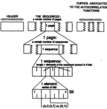
Fig. 7. Data structures concerning the file associated with the functionality of approximated simulation.

The execution time to compute an autocorrelation curve with less than p = 20 points and up to seven oligonucleotides of length s 6 , is ~ 1 seconds, i.e. significantly less than the execution time of 18 seconds (for 200 sequences of length 1000) with the approximated simulation algorithm. Therefore, the exact calculus algorithm is appropriate to compute several thousands of autocorrelation curves with a small number of points (in practice ^20) during a scanning. However, the execution time becomes prohibitive (several minutes or hours) to compute a complete autocorrelation function with 100 points [algorithm in (Kn*) complexity]: in this case, the algorithm of exact calculus must be replaced by the approximated simula-tion one.

Utilities available

Due to the high combination of possible solutions, AGE has been developed to be interactive and user-friendly. It can be used without any computer knowledge as it has several utilities such as: data entries and data modifications by menus; automatic manipulation of files concerning the search, the creation, etc.; graphic tools allowing choices of the number of points in the autocorrelation curve, the number of curves displayed or printed, the color for the curves, the superposition or not of several curves, etc.; PostScript output of text files and figures allowing the use of a broad range of printing devices; display of the execution time according to the constraints chosen, display of the file size, etc.

Data structures

The AGE files are structured according to the functionalities; real, approximated simulation, exact calculus and evolution. For example, the file associated with the functionality of approximated simulation is composed of three parts (Figure 7): (i) the header, which contains the information for the file management and for the type of model (independent, Markov); (ii) the sequences, in particular the nucleotides are stored in 2 bits in order to compress the file; and (iii) the curves associated with the autocorrelation functions; these are stored (to avoid new computations) with a direct access (to get a fast visualization).

Discussion

The software AGE allows the study of a genetic reality, i.e. the identification of statistical properties that are common (or primitive) in genes by applying autocorrelation functions in gene populations, or specific (or actual) to a gene by applying autocorrelation functions in this gene. AGE can simulate this observed genetic reality by models of molecular evolution such as the independent (or Markov) mixing model of primitive oligonucleotides according to given probabilities (or Markov matrix), the random insertion/deletion process of (mono.di, tri)nucleotides, the base mutation process, etc. It is important to stress that AGE can be used both to study a reality and to develop simulation models. This ability is important because a model should be correlated with the reality.

AGE is currently used to generalize our model of DNA sequence evolution (Arques and Michel, 1990b) with auto-correlation functions different from YRY in newly available gene populations (D.G.Arques, C.J.Michel and K.Orieux, in preparation). On the other hand, AGE can be used by biologists without any computer knowledge to identify statistical properties in their newly determined DNA sequences and to simulate (i.e. to explain) their history by models of molecular evolution.

Acknowledgements

We thank Professor Jacques Streith and Nouchine Soltanifar for their advice. Thij work was supported by grants from the Unite1 Associee CNRS no. 822

to D.G.A. and from the Friedrich Miescher Institute to CJ.M. References

Arques,D.G. and Michel.C.J. (1987a) Study of a perturbation in the coding periodicity. Maih. Biosci., 86, 1 — 14.

Arques,D.G. and Michel.C.J. (1987b) A purine-pyrimidine motif verifying an identical presence in almost all gene taxonomic groups. J. Theor. Biot., 128, 457-461.

Arques.D.G. and Michel,CJ. (1987c) Periodicities in introns. Nucleic Acids Res., 15, 7581-7592.

Arques.D.G. and Michel.C.J. (1990a) Periodicities in coding and noncoding regions of the genes. J. Theor. Biol., 143, 307-318.

Arques.D.G. and Michel.CJ. (1990b) A model of DNA sequence evolution. Part 1: statistical features and classification of gene populations. Part 2:

simulation model. Part 3: return of the model to the reality. Bull. Math. Biol., 52, 741-772.

Eigen.M. and Schuster.P. (1978) The hypercycle. A principle of natural self-organization. Part C: the realistic hypercycle. Natunvissenschaften, 65, 341-369.

FickettJ.W. (1982) Rccognilion of protein coding regions in DNA sequences.

Nucleic Acids Res., 10, 5303-5318.

Kimura.M. (1987) The Neutral Theory of Molecular Evolution. Cambridge University Press, Cambridge.

Received on January 21. 1991; accepted on June 6. 1991

Circle No. 2 on Reader Enquiry Card