Neuronal mechanisms for sequential activation of memory items: Dynamics and reliability

HAL Id: hal-02879964

https://hal.archives-ouvertes.fr/hal-02879964

Submitted on 24 Jun 2020

HAL is a multi-disciplinary open access archive for the deposit and dissemination of sci-entific research documents, whether they are pub-lished or not. The documents may come from teaching and research institutions in France or abroad, or from public or private research centers.

L’archive ouverte pluridisciplinaire HAL, est destinée au dépôt et à la diffusion de documents scientifiques de niveau recherche, publiés ou non, émanant des établissements d’enseignement et de recherche français ou étrangers, des laboratoires publics ou privés.

memory items: Dynamics and reliability

Elif Köksal Ersöz, Carlos Aguilar Melchor, Pascal Chossat, Martin Krupa,

Frédéric Lavigne

To cite this version:

Elif Köksal Ersöz, Carlos Aguilar Melchor, Pascal Chossat, Martin Krupa, Frédéric Lavigne. Neuronal mechanisms for sequential activation of memory items: Dynamics and reliability. PLoS ONE, Public Library of Science, 2020, 15 (4), pp.1-28. �10.1371/journal.pone.0231165�. �hal-02879964�

RESEARCH ARTICLE

Neuronal mechanisms for sequential

activation of memory items: Dynamics and

reliability

Elif Ko¨ ksal Erso¨ zID1¤, Carlos Aguilar2, Pascal Chossat1,3, Martin Krupa1,3, Fre´de´ric Lavigne4

1 Project Team MathNeuro, INRIA-CNRS-UNS, Sophia Antipolis, France, 2 Lab by MANTU, Amaris

Research Unit, Route des Colles, Biot, France, 3 Universite´ Coˆte d’Azur, Laboratoire Jean-Alexandre Dieudonne´, Nice, France, 4 Universite´ Coˆte d’Azur, CNRS-BCL, Nice, France

¤ Current address: LTSI, INSERM U1099, University of Rennes 1, Rennes, France *elif.koksal@inria.fr

Abstract

In this article we present a biologically inspired model of activation of memory items in a sequence. Our model produces two types of sequences, corresponding to two different types of cerebral functions: activation of regular or irregular sequences. The switch between the two types of activation occurs through the modulation of biological parameters, without altering the connectivity matrix. Some of the parameters included in our model are neuronal gain, strength of inhibition, synaptic depression and noise. We investigate how these param-eters enable the existence of sequences and influence the type of sequences observed. In particular we show that synaptic depression and noise drive the transitions from one mem-ory item to the next and neuronal gain controls the switching between regular and irregular (random) activation.

Introduction

The processing of sequences of items in memory is a fundamental issue for the brain to gener-ate sequences of stimuli necessary for goal-directed behavior [1], language processing [2,3], musical performance [4,5], thinking and decision making [6] and more generally prediction [7–9]. Those processes rely on priming mechanisms in which a triggering stimulus (e.g. a prime word) activates items in memory corresponding to stimuli not actually presented (e.g. target words) [10,11]. A given triggering stimulus can generate two types of sequences: on the one hand, the systematic activation of the same sequence is required to repeat reliable behav-iors [12–16]; on the other hand, the generation of variable sequences is necessary for the crea-tion of new behaviors [17–21]. Hence the brain has to face two opposite constraints of generating repetitive sequences or of generating new sequences. Satisfying both constraints challenges the link between the types of sequence generated by the brain and the relevant bio-logical parameters. Can a neural network with a fixed synaptic matrix switch behavior between reproducing a sequence and produce new sequences? And which neuronal mechanisms are

PLOS

ONE

Citation: Ko¨ksal Erso¨z E, Aguilar C, Chossat P,

Krupa M, Lavigne F (2020) Neuronal mechanisms for sequential activation of memory items: Dynamics and reliability. PLoS ONE 15(4): e0231165.https://doi.org/10.1371/journal. pone.0231165

Editor: Ste´phane Charpier, Sorbonne Universite

UFR de Biologie, FRANCE

Received: November 6, 2019 Accepted: March 17, 2020 Published: April 16, 2020

Copyright:© 2020 Ko¨ksal Erso¨z et al. This is an open access article distributed under the terms of theCreative Commons Attribution License, which permits unrestricted use, distribution, and reproduction in any medium, provided the original author and source are credited.

Data Availability Statement: All relevant data are

within the manuscript and its Supporting Information files. Code is now available on GitHub viahttps://github.com/elifkoksal/latchingDynamics.

Funding: EKE and MK were supported by the ERC

Advanced Grant NerVi no. 227747. FL was supported by the French government, through the UCAJEDI Investments in the Future project managed by the National Research Agency (ANR) with the reference number ANR-15-IDEX-01.

sufficient for such switch in the type of sequence generated? The question addressed here is how changes in neuronal noise, short-term synaptic depression and neuronal gain make possi-ble either repetitive or variapossi-ble sequences.

Neural correlates of sequence processing involve cerebral cortical areas from V1 [16,22] and V4 [14] to prefrontal, associative, and motor areas [23,24]. The neuronal mechanisms involve a distributed coding of information about items across a pattern of activity of neurons [25–29]. In priming studies, neuronal activity recorded after presentation of a prime image shifts from neurons active for that image to neurons active for another image not presented, hence beginning a sequence of neuronal patterns [30–33]. Those experiments report that a condition for the shift between neuronal patterns of activity is that stimuli have been previ-ously learned as being associated. Considering that the synaptic matrix codes the relation between items in memory [34,35], computational models of priming have shown that the acti-vation of sequences of two populations of neurons rely on the efficacy of the synapses between neurons from these two populations [10,36–39].

Turning to longer sequences, many of the models studied to date rely on the existence of steady patterns (equilibria) of saddle type, which allow for transitions from one memory item to the next [40–42]. Such models are well suited for reproducing systematically the same unidi-rectional sequence: as time evolves neuronal patterns are activated in a systematic order. These works show that the generation of directional sequences relies on the asymmetry of the rela-tions between the popularela-tions of neurons that are activated successively. Regarding the order of populations n, n+1, n+2 in a sequence, the directionality of the sequence is obtained thanks to two properties of the synaptic matrix. First, the synaptic efficacy increases with the order of the populations, that is efficacy is weaker between populations one and two than between pop-ulations two and three [15,40]. Second, the amount of overlap increases with the order of pop-ulations [42]. Indeed, individual neurons respond to several different stimuli [43–45] and two populations of neurons coding for two items can share some active neurons [46,47]. Models have proposed a Hebbian learning mechanism that determines synaptic efficacy as a function of the overlap between the populations [48,49]. In models the amount of overlap codes for the association between the populations and determines their order of activation in a sequence [11,40,42,50]. These works identify sufficient properties of the synaptic matrix to generate systematic sequences. However such properties of the synaptic matrix may not be necessary and neuronal mechanisms may also be sufficient to generate sequences.

Neural network models have pointed to neuronal gain as a key parameter that determines the easiness of state transitions and the stability of internal representations [51]. Further, a cor-tical network model has shown that neuronal gain determines the amount of activation between populations of neurons associated through potentiated synapses [52]. The latter has shown that variable values of gain reproduce the variable magnitude of the activation of associ-ates in memory (semantic priming) reported in schizophrenic participants compared to healthy participants [53–55]. However, these models considered states stability or the amount of activation but not the reliability nor the length of the sequences that can be activated. This points to a possible effect of neuronal gain but leaves open the possibility that it could play a role in the regularity or variability of the sequences that can be activated.

In this work we consider the case of fixed synaptic efficacy and fixed overlap to focus on sufficient neuronal mechanisms that underlie the type of sequence, reliable or variable. The present study mathematically analyses a new and more general type of sequences in which the states of the network do not need to pass near saddle points. The model is based on a more general mechanism of transition from one memory item to the next, with the saddle pattern replaced by a saddle-sink pair (see [56], for a prototype of this mechanism of transition). As time evolves the sink and saddle patterns become increasingly similar, so that even a small

Competing interests: The authors have declared

random perturbation can push the system past the saddle to the next memory item. In the model those new dynamics alleviate constraints on the synaptic matrix by allowing sequences that form spontaneously with the transitions obtained between populations related through fixed overlap, without theoretical or practical restriction on the length of the sequences. We show that, in addition to regular (predictable) sequences which follow the overlap between the populations, our system also supports sequences with random transitions between learned pat-terns. We investigate how changes in parameters with a clear biological meaning such as neu-ronal noise, short-term synaptic depression (or short-term depression (STD), for short) and neuronal gain can control the reliability of the sequences.

Our model is mainly deterministic, however small noise is needed to facilitate transitions from one state to the next. As in [40] we used small noise to activate regular transitions, and, unlike in other contexts, e.g. [42], we used small noise for random activations. In the context of large noise (stochastic systems), it is difficult to generate regular sequences if white noise is used. This is the main reason why we decided to take an almost deterministic approach. As our goal was to understand the possible effects of deterministic dynamics, we chose time inde-pendent white noise.

Model

The focus of this paper is to present a mechanism of sequential activation of memory items in the absence of either increasing overlap, or increasing synaptic conductance, or any other fea-ture forcing directionality of the sequences. We present this mechanism in the context of a simple system, however the idea is general and can be implemented in detailed models. We use the neural network model of the form

_ xi ¼xið1 xiÞð mxi I l P_N j¼1xjþ P_N j¼1J max i;j sjxjÞ þ Z ð1Þ _si ¼ 1 si t_r Uxisi ði ¼ 1; � � � ; NÞ; ð2Þ as in [40], with the variablesxi2 [0, 1] representing normalised averaged firing rates of

excit-atory neuronal populations (units), andsi2 [0, 1] controlling STD. The limiting firing rates

xi= 0 andxi= 1 correspond respectively to the resting and excited states of uniti. Any set

(x1, . . .,xN) withxi= 0 or 1 (i = 1, . . ., N) defines a steady, or equilibrium, pattern for the

net-work. In the classical paradigm the learning process results in the formation of stable patterns of the network. Retrieving memory occurs when a cue puts the network in a state which belongs to the basin of attraction of the learned pattern.Eq (1)is usually formulated using the activity variableui(average membrane potential) rather thanxi, andxiis related touithrough

a sigmoid transfer function. Our formulation in which the inverse of the sigmoid is replaced by a linear function with slopeμ, was shown to be convenient for finding sequential retrievals

of learned patterns, see [40].

The parameters inEq (1)areμ (or its inverse γ = μ−1which is the gain, supposed identical, of the units, or slope of the activation function of the neuron [57]),λ the strength of a non-selective inhibition (inhibitory feedback due to excitation of interneurons) andJmax

i;j the

maxi-mum weight of the connexion from unitj to unit i. The parameter I can be understood as

feed-forward inhibition [58] or distance to the excitability threshold. This parameter was used by [11,40,50]. Note thatI controls the stability of the completely inactive state (xi= 0 for alli). In

this work we setI to 0, which means that the inactive state is marginally stable (see Section

“Marginal stability of the inactive state” inS1 Appendix). This is reminiscent of the up state [59], characterised by neurons being close to the firing threshold. Finally,η is a noise term

which can be thought of as a fluctuation of the firing rate due to random presence or suppres-sion of spikes. In our simulations we considered white noise with the additional constraint of pointing towards the interior of the interval [0, 1]. Other types of noise can be chosen, this does not affect the mechanisms which we have investigated.

STD reported in cortical synapses [60] rapidly decreases the efficacy of synapses that trans-mit the activity of the pre-synaptic neuron. This is modeled byEq (2)whereτris the synaptic

time constant of the synapse andU is the fraction of used synaptic resources. In order to be

more explicit for the rest of the manuscript, we re-writeEq (2)as

t_r_s_i ¼ 1 si rxisi ði ¼ 1; � � � ; NÞ; ð3Þ whereρ = τrU.Eq (3)immediately shows the respective roles played byτrand the synaptic

productρ. The synaptic time constant τrproduces slow dynamics whenτr� 1, whileρ

deter-mines the value of the limiting state of the synaptic strength. More precisely, for an active unit

xi= 1 with initially maximal synaptic strengthsi= 1,sidecays towards the valueS = (1 + ρ)−1

by following

siðtÞ ¼ 1

1 exp ð ð1 þ rÞt=trÞ

1 þ r ;

with the decay time constant (1 +ρ)/τrwhich depends onτr. For an inactive unitxi= 0,si

recovers tosi= 1 by following

siðtÞ ¼ 1 ð1 sið0ÞÞexp ð t=trÞ;

with the recovery time constantτrandsi(0) is the synaptic value at the beginning of the

recov-ery process.

The main difference in the model between this paper and [40] is the form of the matrix of excitatory connectionsJmax:

Jmax_¼ 1 1 0 . . . 0 1 2 1 .. . ... 0 .. . .. . .. . 0 .. . . . . 1 2 1 0 . . . 0 1 1 2 6 6 6 6 6 6 6 6 6 6 6 6 4 3 7 7 7 7 7 7 7 7 7 7 7 7 5 N�N : ð4Þ

This matrix is derived by the application of the simplified Hebbian learning rule of [61] (details provided in [40]) using the collection of learned patterns

xi¼ ð0; � � � ; 0; 1; 1; 0; � � � ; 0Þ ; i ¼ 1; � � � ; P ð5Þ

where the two excited units arei and i + 1. Conditions for the stability of these patterns in the

absence of STD were derived in [40]. Note that the overlap betweenξiandξi+1is constant (one unit). By the application of the learning rule the coefficients ofJmaxare given by the formula:

Jmax i;j ¼

XP

k¼1

xk_ixk_j: ð6Þ

Consequently the matrixJmaxis made up of identical (1 2 1) blocks along the diagonal, so that there is no increase in either overlap or the synaptic efficacy (weight) along any possible

chain. We prove mathematically and verify by numerics thatEq (1)admits a chain of latching dynamics passing through the patternsξi,i = 1, . . .n − 2, either in forwards or in backwards

direction depending on the activation, as well as shorter chains. The simplest way to switch dynamically from the learned patternξitoξi+1is by having a mechanism such that uniti passes

from excited to rest state, then uniti + 2 passes from rest to excited state. STD can clearly result

in the inhibition of uniti. However in the framework of [40] it was not possible to obtain the spontaneous excitation of uniti + 2 with the connectivity matrixEq (4), because it was required that the upper and lower diagonal coefficients ofJmaxbe strictly increasing with the orderi.

Connectionist models have shown the effects of fast synaptic depression on semantic mem-ory [62] and on priming [11,50]. Recall that fast synaptic depression is one of the aspects of short term synaptic plasticity [63]. For the sake of simplicity, we neglect the other aspects of short term synaptic plasticity, but their effects on sequential activation of memory items are likely to be significant [64], and we intend to investigate them in further work. Fast synaptic depression contributes to deactivation of neurons initially active in a pattern—because they activate less and less each other—in favor of the activation of neurons active in a different but overlapping pattern—because newly activated neurons can strongly activate their associates in a new pattern. The combination of neuronal noise and fast synaptic depression enables latch-ing dynamics in any direction dependlatch-ing on the initial bias due to random noise. Indeed, when the parameters lie within a suitable range, the action of STD has the effect of creating a “dynamic equilibrium” with a small basin of attraction. This dynamic equilibrium could beξi, ^

xi_{(the pattern in which only uniti + 1 is excited) or an intermediate pattern for which the} value ofxiis between 0 and 1. Subsequently the noise allows the system to eventually jump to

ξi+1, the process being repeated sequentially between all or part of the learned patterns. This noise-driven transition is what we call anexcitable connection by reference to a similar

phe-nomenon discussed in [56]. Chains of excitable connections can also be activated or termi-nated by noise. Last but not least we show that our system, depending on the value of the parameterμ, hence of the neuronal gain γ = 1/μ, will follow the sequence indicated by the

over-lap or execute a random sequence of activations. Changes in neuronal gain change the sensitiv-ity of a neuron to its incoming activation [57,65,66], and are reported to impact contextual processing [67] to enhance the quality of neuronal representations [68] and to modulate

acti-vation between populations of neurons to reproduce priming experiments [52]. Here we show

how changes in neuronal gain switches the network’s behavior between repetitive (reliable) sequences and variable (new) sequences.

We proceed to present the results in more detail, as follows. In Sec. Case study: a system withN = 8 excitable units we present simulations for the network with N = 8, which serves as

an example of the more general construction. In Sec. Case study: a system withN = 8 excitable

units we sketch the methods we use to search for or verify the existence of the chains. In Sec. Irregular chains and additional numerical results we discuss irregular chains of random activa-tions versus regular chains defined by the overlap. Simulaactiva-tions were run using the Euler-Mar-uyama method with time steps of 0.01 ms.

Results

Case study: A system with

N = 8 excitable units

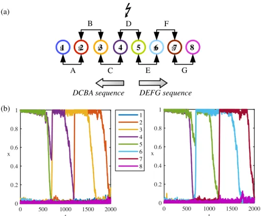
We consider sequences of seven learned patternsξ1, . . .,ξ7(named ABCDEFG) encoded by eight unitsx1, . . .,x8. The sequence represents the sequential activation of pairs of units 1-2, 2-3, 3-4, 4-5, 5-6, 6-7 and 7-8, corresponding to patterns A and B, B and C, etc. with an overlap of one unit between them (seeFig 1a). Learning is reported to rely on changes in the efficacy

of the synapses between neurons [69] through long term potentiation (LTP) and long term

depression (LTD) [70–72]. As a consequence, LTP/LTD potentiates/depresses synapses

between units coding for patterns as a function of their overlap, that is synapses between units coding for overlapping patterns are more potentiated. Due to the constant overlap, all synapses between overlapping patterns are equal. Note that the matrixJmaxis learned as a function of the overlap between patterns without imposing any sequences. A consequence is that learning of independent pairs of patterns generates a matrix that allows for the activation of sequences. A system ofN = 8 excitatory units can encode P = N − 1 = 7 regular patterns in Jmax(seeFig

1a). Encoded memory items can be retrieved either spontaneously (in a noisy environment) or

when the memory network is triggered by an external cue [42,73]. Unitsx1andx8are the least self-excited units withJmax

1;1 ¼J8;8max¼ 1, thus it is very unlikely to active them unless they are part of the initial activity state. Hence, the longest chain hasP − 1 = 6 consecutive patterns.

Directional sequences from a stimulus-driven pattern in the sequence. Starting from the first pattern A, the directional activation corresponds to the sequence ABCDEFG (Fig 1b

left panel). The forward direction is imposed byJmaxbecausex1is less excited sinceJ1;1max¼ 1. Hence, while the synaptic variabless1ands2are equal and decreasing together as the system lies in the vicinity ofξ1,x1is deactivated beforex2. In the same interval of times2<s3ands2−

s3increases so thatx2becomes unstable beforex3and the system now may converge toξ2. The process can be repeated betweenξ2andξ3etc. Similarly, starting from the last pattern G gives the reverse direction (GFEDCBA) to the system (Fig 1bright panel).

Initialising the system from a middle patternξidoes not introduce any direction, since the two active units ofξiare equally excited. While their synaptic variables are decreasing together,

Fig 1. Directional sequences of an endpoint stimulus-driven system. (a) Each numbered circle represents a unit.

Consecutive units encode a pattern. Except forx1andx8, each unit participates in two patterns. A forward sequence is

the activation of units in increasing order. A backward sequence is the activation of units in decreasing order. (b) Left panel: System initialised from the pattern A follows the forward sequence until the pattern F. Right panel: System initialised from the pattern G follows the backward sequence until the pattern B. Same colour code is used to represent units’ indices in (a) and (b). Parameters:μ = 0.41, λ = 0.51, I = 0, ρ = 1.8, τr= 900,η = 0.02.

depending on the noise at the moment whenξibecomes unstable, eitherξi−1orξi+1is activated with equal probabilities.Fig 2shows the response of the system starting from a mid-point

pat-tern D. The activated sequence can go in either direction DEFG or its reverse DCBA. The

ran-dom choice for a sequence is driven by a bias in the noise at the time of stimulus-driven

activation of the mid-point pattern.

Noise-driven random sequence from a mid-point pattern in the sequence. The units that participate in two patterns (overlapping units) have stronger self-excitation as it is mani-fested by the diagonals ofJmax. These units (xi,i 6¼ {1, 8}) are likely to be excited by random

noise and they can activate others which they encode a pattern with. After a patternξior the associated intermediate pattern ^xi_{¼ ð0; . . . ; 0; 1; 0; . . . ; 0Þ being randomly excited by noise,} the system can follow eitherξi−1orξi+1. The robustness of activity depends on the system

parameters.Fig 3shows an example of spontaneous activation of a mid-point pattern D where

the directional oriented sequence can be either DEFG or its reverse DCBA. Similar to the sys-tem initialised from a middle pattern, therandom choice for a direction is driven by a bias in

the noise at the time of noise-driven activation.

Sensitivity of the dynamics upon parameter values. We have seen that patterns can be retrieved sequentially when the system is triggered by a cue or spontaneously by noise. How-ever the effectiveness of this process depends on the values of the parameters in Eqs(1)and

(2). The dynamics of the system can follow part of the sequence, then either terminate on one

Fig 2. Directional sequences of a midpoint stimulus-driven system. (a) Each numbered circle represents a unit.

Consecutive neurons encode a pattern. Except forx1andx8, each unit participates in the encoding for two patterns.

When the system initialised from the pattern D, it follows either the “DCBA” or “DEFG” sequence. (b) Left panel: System initialised from the pattern D follows the “DCBA” sequence until the pattern B. Right panel: System initialised from the pattern D follows “DEFG” sequence until the pattern F. The same colour code is used to represent units’ indices in (a) and (b). Parameters:μ = 0.414, λ = 0.51, I = 0, ρ = 1.8, τr= 900,η = 0.02.

https://doi.org/10.1371/journal.pone.0231165.g002

patternξiwithi < N − 1, or converge to a non learned pattern. Moreover we identified two

dif-ferent dynamical scenarios by which a sequence can be followed, depending mainly on the

value ofμ. This will be analyzed in Sec. Analysis of the dynamics. Here we comment on

numerical simulations which highlight the dependency of the sequences upon parameter values.

The behavior of the model was tested on simulation data by measuring the length of regular sequences generated by the network (chain length) and by computing the distance made from the initial pattern after irregular sequences (distance). Chain length and distance were analyzed by fitting linear mixed-effect models (LMM) to the data, using the lmer function from the lme4 package (Version 1.1–7) in R (Version R-3.1.3 [74]). All predictor parameters (inverse of the gainμ, inhibition λ, time constant τr, synaptic constantρ and noise η) were defined as

con-tinuous variables and they were centered on their mean. The optimal structure was determined after comparing the goodness of fit of a range of models, using Akaike’s information criterion (AIC); the model with the smallest AIC was selected, corresponding to the model with main effects and interactions between all of the parameters. The significance of the effects was tested using the lmerTest package. For the sake of clarity of the text, we flag the levels of signifi-cance with one star (�) if p-value <0.05, two stars (��) if p-value <0.01, three stars (���) if p-value<0.001.

Fig 4shows time series of the full or partial completion of sequences of retrievals (forN = 8

units) for two different values of noise amplitudeη = 0.02 (first row) and η = 0.04 (second and third row). In each case the two first columns show time series with the STD parametersρ =

1.8 andτr= 300 while the last column corresponds to the choiceρ = 1.8 and τr= 900. By fixing

the synaptic constantρ = 1.8, we ensure that the synaptic variables sidecay to the same valueS

with a decay time depending onτr(see Sec.Model). The global inhibition coefficientλ is set at

0.51 in rowsFig 4a and 4bandλ = 0.56 in rowFig 4c. For each choice of the STD parametersμ

takes two values, eitherμ = 0.41 or μ = 0.21.

Observe that the sequence and the pattern durations are shorter in the system with fast syn-apses (τr= 300) than the one with slow synapses (τr= 900). In the case of weaker noise (Fig 4a)

and fast synapses, the system follows the sequence ABCDEF whenμ = 0.41 whereas it stops at

the pattern B whenμ = 0.21. In other words, increasing μ (decreasing neural gain) in the

sys-tem with fast synapses recruits more units sequentially. Another way to increase the chain length forμ = 0.21 is slowing down the synaptic variables. The system with slow synapses can Fig 3. Directional sequences of a spontaneously activated system. System activated spontaneous by random noise

can move in backward (a) or forward (b) directions. Parameters:μ = 0.21, λ = 0.51, I = 0, ρ = 1.8, τr= 300,η = 0.04.

follow the sequence ABCDEF for a wide range ofμ values. In fact the two different values of μ

inFig 4correspond to the two different dynamical scenarios which have been evoked in the beginning of this section. This point will be developed in Sec. Analysis of the dynamics. When noise is stronger (Fig 4b) the picture is different: the full sequence can be completed with fast synapses even forμ = 0.21. However, the sequence is shorter with slow synapses and the system

quickly explores unexpected patterns like one with three excited units 2, 3, 4 aroundt = 600

(which is not a learned pattern) in third panel ofFig 4b. These type of activity can be observed for a wide range ofμ values with slow synapses.

Fig 4. Response of the system initialised from pattern A (units 1-2) to different levels of noiseη and system

parametersλ, μ, τr. Synaptic variables are faster along the first two columns (τr= 300) than the last column (τr= 900).

In all simulationsI = 0. Row (a) η = 0.02, λ = 0.51. The system with fast synapses can follow the longest sequence from

A (units 1-2) to F (units 6-7) forμ = 0.41 (the first panel) but not for μ = 0.21 (the second panel), while the slow

synapses can trigger the longest sequence (the third panel). Row (b)η = 0.04, λ = 0.51. Increasing the noise amplitude enables the activation of the whole sequence with fast synapses (the first two panels), whereas the slow synapses give either very short patterns or 3 co-active units, the third panel, respectively. Row (c)η = 0.04, λ = 0.56. Increasing the

global inhibitionλ regulates the transition for slow synapses (the third panel), whereas the system with fast synapses andμ = 0.41 (the first panel) randomly activates learned patterns and yields short regular and irregular sequences. On

the other hand, the system withμ = 0.21 and fast synapses (the second panel) can preserve a regular sequence. https://doi.org/10.1371/journal.pone.0231165.g004

Comparison betweenFig 4b and 4cexemplifies the effect of changing inhibitionλ and μ (inverse of neural gain) for the same noise amplitude. Increasing the inhibition coefficientλ regulates the transition for slow synapses, while fast synapses and high values ofμ (low neural

gain) randomly activates the learned patterns and yields short sequences. The latter is also due to the self inhibition in the system given by the−μxiterm inEq (1)which facilitates

deactiva-tion of an active unit, but makes difficult for an inactive unit to be activated if it is too high. Notice the self inhibitory effect in the fast synapses can be compensated for slow synapses and smallμ (high neural gain) which can regularize sequences.

Length of a chain. When the patterns in a chain are explored in the right order by the sys-tem we call itregular. As we saw in Sec. Sensitivity of the dynamics upon parameter values it

can happen that only part of the full regular chain has been realised before it stops or starts exploring patterns in a different order, hence activating an irregular chain. We call the partial regular chain aregular segment and its length is the number of patterns it contains. Here we

investigate the maximal length that a regular segment starting at pattern A can attain. This length is the rank of the last activated pattern over simulations. It depends on noiseη but also on the neuronal parameters (μ, λ) and on the synaptic parameters (τr,ρ). As it can be read in Eq (3),ρ characterizes the limiting decay state of the synaptic variable. Possible impact of τr

andρ on the dynamics has been investigated in [40]. It has been shown in a system with a a structured connectivity matrix that deactivation of a unit is harder forρ being small while too

highρ prevents recruiting new units. Thus, ρ determines the reliability of a sequential

activa-tion. On the other hand, the threshold of the noise need for activation of a chain decreases with increasingτrforρ constant.

The relation between the model parameters and the sequential activation is more subtle with the learning matrix(4)derived from the most simplified Hebbian learning rule than a structured one as in [40]. In Figs5and6we present the mean chain length for two different noise intensities;η = 0.02 and η = 0.04, respectively. In each figure synaptic parameters are ρ 2 {1.2, 2.4},τr2 {300, 900}. Neural parametersλ and μ are varied within a range assuring the

exis-tence of chains of at least length 2. Details of the sequences are shown inS1andS2Figs. Statis-tics on chain length show main effects of each parameter (η (���_{),μ (}��_{),λ (}���_),τ

r(���) and

ρ (���

). They also show an interaction between the five parameters altogether (���).

In all panels ofFig 5whereη = 0.02, the average chain length increases with μ, unless μ is too large. InFig 5a and 5bwe observe a sharp increase in the chain length forλ = {0.551, 0.601} (less pronounced forλ = {0.501, 0.651}). The sharp increase in the average chain length

occurs when the bifurcation scenario changes aroundμ � μ�

(for the definition ofμ�

see Sec.

Analysis of the dynamics and section “Dynamic bifurcation scenarios” inS1 Appendix) While

middle range inhibition leads to longer sequences forρ = 1.2, weak inhibition is more suitable

forρ = 2.4 (Fig 5c and 5d). Indeed,λ and ρ have interacting effects on chain length (���_).

InFig 6, the noise level is increased toη = 0.04. Generally speaking, increasing the noise level prolongs the chains by facilitating the activation. Especially forτr= 900 andλ = 0.651, the

average chain length is considerably higher withη = 0.04 (Fig 6) thanη = 0.02 (Fig 5). On the other hand, the relation between the average chain length andμ becomes more delicate. InFig 6a and 6bforρ = 1.2, the average chain length peaks for the intermediate values of μ. Strong

inhibitionλ = 0.651 prolongs the chains for small values of μ and slow synapses, whereas inter-mediate values of inhibitionλ = {0.551, 0.601} favor longer chains as μ increases. For ρ = 2.4 (Fig 6c and 6d) chains are longer under weak inhibitionλ = 0.501. However, increasing μ under weak inhibition considerably shortens the chains. The average chain length increases withμ under strong inhibition for λ = {0.601.0.651} Parameters λ and μ have interacting effects

Our analysis unveils a nonlinear relation betweenμ and the chain length. When μ is small,

an increase ofμ provokes an increase of the length of the chain. However, in most cases we

find that the chain lengths are maximal for intermediate values ofμ. This is clear intuitively:

large gain (smallμ) prevents the units from deactivating, making the transition from one

pat-tern to the next difficult. Small gain, on the other hand, prevents the next unit from activating. Another factor is the occurrence of the transition from scenario 1 to 2 (see Sec. Analysis of the

dynamics and section “Dynamic bifurcation scenarios” inS1 Appendix). The synaptic product

ρ and the global inhibition parameter λ also influence the system’s behaviour. For ρ = 1.2,

inhi-bition in the middle range leads to longer sequences, whereas weak inhiinhi-bition is more suitable forρ = 2.4.

Analysis of the dynamics

Latching dynamics is defined as a sequence (chain) of activations of learned patterns that de-activate due to a slow process (e.g., adaptation, here synaptic depression), allowing for a transi-tion to the next learned pattern in the sequence [11,75]. Here we refine this description using

Fig 5. Average chain length in a regular segment for noiseη = 0.02. Synaptic time constant equals to τr= 300 on

panels (a) and (c), andτr= 900 on panels (b) and (d). (a, b) Activity forρ = 1.2. The chain length increases with μ (1/

neural gain) andτr. The global inhibition value,λ, should be high enough for a sequential activation, but the chain

length decreases ifλ is too high. (c, d) Activity for ρ = 2.4. The chain length increases with μ and τr, but decreases with

λ. SeeS1 Figfor the details of the activity.

https://doi.org/10.1371/journal.pone.0231165.g005

the language of dynamics and multiple timescale analysis. The main idea is to treat the synaptic variablessiasslowly varying parameters, so that the evolution of the system becomes a movie of

the dynamical configurations of the unitsxi. On the other hand the firing rateEq (1)is well

adapted to analyze latching dynamics. Indeed, from the form ofEq (1)(assuming for the

moment that noise is set to 0) one can immediately see that wheneverxiis set to 0 or 1, this

variable stays fixed at any time. Therefore considering any face in the hypercube [0, 1]N defined by two coordinates (xi,xj), the other coordinates being fixed at 0 or 1, it is invariant

under the flow ofEq (1). In other words, any trajectory starting on the face stays entirely on it. This is of course true also for the edges and vertices at the boundary of each face. Each vertex is

an equilibrium ofEq (1)and connections between such equilibria can be realised through

edges of the hypercube, which greatly simplifies the analysis.

When the couple (xi,si) of uniti is set at (1, 1), xiis fixed as we have seen but STDEq (3)

induces an asymptotic decrease of the synaptic variable towards the valueS = (1 + ρ)−1. This in turn weakens the synaptic weightJmaxsiinEq (1), which may destabilizeξiin the direction of

Fig 6. Average chain length in a regular segment for noiseη = 0.04. Synaptic time constant equals to τr= 300 on

panels (a) and (c), andτr= 900 on panels (b) and (d). (a, b) Activity forρ = 1.2. The chain length increases with τr.

Chains are longer for intermediate values ofμ (intermediate values of neural gain), but shorter for μ too high (low

neural gain). Increasing inhibitionλ facilitates regular pattern activation for the low values of μ, see for instance λ = 0.501 vsλ = 0.601 in (a), but ceases if it is too strong. (c, d) Activity for ρ = 2.4. The chain length increases with τr, but

decreases withλ. Increasing μ lengthens the chains more with τr= 900 thanτr= 300. SeeS2 Figfor the details of the

activity.

^

xi_{. Considerings}

ias a slowly varying parameter this can be seen as adynamic bifurcation of an

equilibrium along the edge fromξito ^xi_{. The following scenario was described in [40]. For the} sake of simplicity we now assumei = 1 (the same arguments hold for any i). The patterns ξ1

, ^x1 andξ2lie at the vertices of a face, which we call F, generated by the coordinatesx1andx3, with

x2= 1 and the rest of the coordinates being set to 0.

Fig 7shows three successive snapshots of the movie on F. The left panel illustrates the ini-tial configuration, with the stable patternξ1

corresponding to the top left vertex. Then at some timeT0an equilibrium bifurcates out of ^x1in the direction ofξ1(here the ‘slow’ STD time plays the role of bifurcation parameter, see middle panel). After a timeT1(right panel) this bifurcated equilibrium disappears inξ1which becomes unstable and a connecting trajectory is created along the edge with ^x1_{. Simultaneously a trajectory connects ^x}

1toξ2along the corre-sponding edge. It results that the following sequence of connecting trajectories is created: x1! ^x1 _{! x}2

. As a result, any state of the system initially close toξ1will follow the ‘vertical’ edge towards ^x1_{, then the ‘horizontal’ edge towardsξ}

2. The process can repeat itself fromξ2to

ξ3and so on. It was shown in [40] that in order to work, this scenario requires that the coeffi-cients of the matrixJmaxsatisfy the relationJmax

1;2 <J2;3max(more generallyJi;iþ1max <Jiþ1;iþ2max ,i = 1, . . .,

P − 1, for the existence of a chain of P patterns), a condition which does not hold withEq (4). The results of this paper rely on the observation that the existence of the connections x1 ! ^

x1 _{! x}2

fort > T1(right panel ofFig 7) is not needed for the occurrence of chains. We will show below that for the connectivity matrixJ given byEq (4)the connections exist for at most a unique value oft = T1and yet regular chains or segments can occur. Fort > T1the connect-ing trajectory along the edge ^x1

x2is broken by a sink (stable equilibrium) close to ^x1 . In such case strong enough noise perturbations could push a trajectory out of the basin of attrac-tion of the sink to the basin of attracattrac-tion ofξ2. As a result the trajectory would get past ^x1_and converge towardsξ2, as expected. When such chains driven by noise exist, we call them excit-able chains by reference to [57] who introduced the concept. In the case when the connections exist fort = T1chains occur with noise of arbitrarily small amplitude, because ast approaches

Fig 7. Representative phase portraits of the fast dynamics on the face F corresponding to the scenario of [40]. The

phase portraits are shown at three different ‘slow’ STD times. Green, orange and purple dots represent the stable, completely unstable and saddle equilibria, respectively. The blue lines illustrate segments of trajectory starting nearξ1_.

(a) The learned patternsξ1_and

ξ2_{are stable for}

t < T0. (b) The bifurcation of a saddle point on the edge betweenξ1and

^

x1_{happens for}

T0<t < T1. (c) Patternξ1has become unstable along the edge x 1 _^

x1_whilst

ξ2_{is still stable for} t > T1.

The saddle point in the interior of F merges with the bifurcated equilibrium before (c) is realised.

https://doi.org/10.1371/journal.pone.0231165.g007

T1from above the amplitude of noise needed to jump over to the basin of attraction ofξ2 con-verges to 0. We extend the terminologyexcitable chain to this case also.

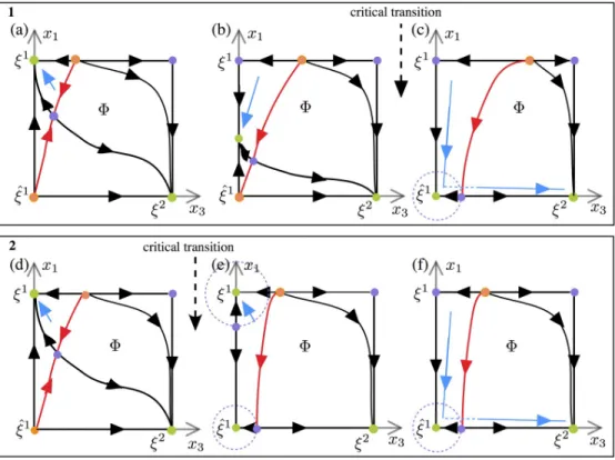
Under this new scheme of excitable chains the number of possible transitions is much larger and multiple outcomes are possible. We have identified two scenarios (named 1 and 2) by which these excitable chains can occur in our problem. Typical cases are illustrated onFig 8. As inFig 7, snapshots of the dynamics at three different “slow” times are shown. The red line marks the boundary of the basin of attraction ofξ2and the dashed circles mark the closest distances for a possible stochastic jump out of it. In both scenarios a completely unstable

equi-librium point exists on the edge fromξ1to the unnamed vertex on F, which corresponds to

the pattern (1, 1, 1, 0, . . ., 0) (not a learned pattern).

Under Scenario 1 the patternξ1first loses stability by a dynamic bifurcation of a sink (stable equilibrium) along the edge x1 ^x1_{. The trajectory, which was initially in the basin of} attrac-tion ofξ1, follows this sink while it is traveling along the edge x1 _^

x1_{towards ^x}1_{(Fig 8b). In} this time interval the distance between the sink and the attraction boundary ofξ2(the red line inFig 8b) is decreasing. Hence it becomes more likely for the noise to carry the trajectory over theξ2stability boundary, activating a transition toξ2. The noise level necessary for the jump becomes smaller as the sink approaches ^x1_{. The critical transition shown inFig 9aoccurs as}

Fig 8. Phase portraits of the fast dynamics on the face F at three different ‘slow’ STD times. Stable patterns are

coloured in green. The red trajectories are separatrices between the basins of attraction of the stable equilibria. The blue lines illustrate segments of a trajectory starting nearξ1_{. Box (1) panels (a,b,c) Phase portraits illustrate the}

mechanisms that can lead to transitionξ1_!

ξ2_{with excitable connections in Scenarios 1 as time evolves. (a) Trajectory}

starting nearξ1_{converges to}

ξ1_{. (b) Trajectory follows the saddle between}

ξ1_{and ^x}1_{on the}

x1-axis. (c) Trajectory

“jumps” out of the basin of attraction of ^x1_{under the effect of noise and converges towards}

ξ2toξ1. Box (2) panels (d,e, f) Phase portraits illustrate the mechanisms that can lead to transitionξ1_!

ξ2_{with excitable connections in Scenarios}

2 as time evolves. (d) Trajectory starting nearξ1_{converges to}

ξ1_{. (e) Trajectory remains in the basin of attraction of} x1

defined by the saddle on thex1-axis. (f) Trajectory “jumps” out of the basin of attraction of ^x1under the effect of noise

and converges towardsξ2_.

the sink reaches ^x1. At this moment, noise of arbitrarily small amplitude can cause the transi-tion. Subsequently ^x1is transiently stable and the distance to theξ

2

attraction boundary increases. Therefore, it becomes likely that the trajectory remains trapped in the basin of attraction of ^x1_{, as shown inFig 8c). A further decrease ofs}

2occurring with the passage of time gives a loss of stability of ^x1_{and the trajectory leaves F to the inactive state. This is the} mechanism of the termination of the regular part of the chain (seeFig 2for an example).

In Scenario 2 the overlap equilibrium point ^x1_{becomes a stable beforeξ}1

loses stability. At the critical transition (Fig 9b), a sequence of connections fromξ1

toξ2

does not exist, hence the trajectory cannot pass fromξ1toξ2unless the noise is sufficiently large. In the context of this scenario regular chains tend to be substantially shorter.

As we have described above, noise is indispensable for crossing the attraction boundary of the next pattern, hence it is crucial for the chains we study. Minimum noise level required for jumps is scenario dependent. In Scenario 1, ass1ands2decrease along the trajectory, the dis-tance between the sink and theξ2attraction boundary also decreases, becoming arbitrarily small as the critical transition is approached. Thus the noise amplitude required for a jump also decreases to 0. In Scenario 2 noise needs to be stronger to make the trajectory cross over the excitability thresholds ofξ1and ^x1_{. On the other hand, we should also keep in mind that} too strong noise can hinder regular chains. Simulations (and analysis, seeS1 Appendix) iden-tifyμ as the main control parameter which determines the choice between these scenarios: the

system follows Scenario 1 for higher values ofμ and Scenario 2 for lower values of μ. This

explains the difference in behavior seen inFig 4at lower and higher values ofμ. The boundary

between the two regions is defined by the valueμ = μ�_{for whichξ}1

and ^x1_{change stability at} the same time. For an analytic definition ofμ�_{and more detailed analysis, seeS1 Appendix. In} the next section we will see how these scenarios affect irregular activation.

Fig 9. Phase portraits corresponding to critical transitions in Scenario 1 and Scenario 2. These phase portraits

occur for a special value ofσ such that ^x1_{changes from a saddle to a sink. (a) The phase portrait of the critical}

transition corresponding to Scenario 1 contains a sequence of connecting trajectories fromξ1toξ2, allowing for a transition fromξ1toξ2with arbitrarily small noise (e.g. forρ = 2.4, τr= 900,λ = 0.55, μ = 0.45, the critical transition

occurs ats1� 0.45,s2� 0.56). (b) In the phase portrait of the critical transition corresponding to Scenario 2, a

transition fromξ1_to

ξ2_{would fail unless the noise amplitude is sufficiently large. (e.g. for}

ρ = 2.4, τr= 900,λ = 0.55, μ =

0.15, the critical transition occurs ats1� 0.37,s2� 0.49). https://doi.org/10.1371/journal.pone.0231165.g009

Irregular chains and additional numerical results

The question we address here is what happens after the last pattern of a regular segment has been reached. We let (i, i + 1) denote the last pattern of the regular sequence. It follows from

previous analysis that the trajectory will remain near ^xi_{for a considerable amount of time.} Subsequently ^xi_{can lose stability and the trajectory passes to the inactive state, or ^x}i_remains stable indefinitely. By our choice of parameters (settingI = 0, see Sec.Model) the inactive state is marginally stable, which means that an irregular activation will eventually happen due to small noise and a the next pattern will be chosen at random. The mechanism of random activa-tion from ^xi_{, is similar, with the exception that chain reversal is likely to occur in this case. The} transition time to an irregular activation may be significantly longer than in the case of regular transitions, which allows for the recovery of the synaptic variables.Table 1assembles the fea-tures of regular and irregular activations, as predicted by the analysis.

Our numerical results confirm the trends of the analytical predictions, at the same time showing that the dynamics of the model is more complex and other parameters play a very important role. In particular, interestingly, the longest regular segments are observed forμ

val-ues corresponding to scenario 1 close toμ = μ�_{, which is the boundary value separating}

scenar-ios 1 and 2 (see Sec. Analysis of the dynamics). Regular segments typically become shorter ifμ

is increased significantly beyondμ�_{, see Figs5and6. This means that there exists an optimalμ}

window for the existence of long regular segments, or, in other words, neuronal gain needs to be not too small and not too large.

In this section we will discuss features of irregular activation, based on numerical results. To show statistics of irregular activation we define a measure of ‘distance’Δ, as follows. Sup-pose at a timet, xpandxqare the two most recently activated units, withxpprecedingxqin its

activation. We define

D ¼q p:

Note that a regular chain satisfiesΔ = 1 for all t until the last pattern is reached. We distinguished two cases of irregular continuation of chains: reversing the chain (Δ = −1) and random reactivation of new chains (Δ 6¼ −1). We allow the possibility of Δ = 1 as such chains can occur in an irregular way for the following reason: an irregular activation is typically preceded by a complete deactivation, usually with a prolonged passage time. The new activation is random, so that an activation to the pattern which is next in the overlap sequence can occur, for instance the sequence [1, 2]![2]![] ! [3]![2, 3]. . .. Such reactivations are documented in details inS3andS4Figs.

Recall the scenarios 1 and 2 for transitions from one pattern to the next (Fig 8). The former occurs for “large” values ofμ and the latter for lower values of μ. Let ^xp_{be the last intermediate} state at the end of the regular segment. In Scenario 2 either ^xp_{remains stable indefinitely or it} destabilizes after some (long) time due to the repotentiation ofsp. The latter case corresponds

to a dynamic scenario for a chain’s reversal. We refer to the prolonged residence of the system

Table 1. Features of regular and irregular transitions as predicted by the analysis of Sec. Analysis of the dynamics. Cognitive function Regularity Dynamic mechanism

Predicted sequence of activation of learned patterns

Deterministic behaviour Dynamic bifurcation, mostly scenario 1, computable transition time by integration Irregular activation of

learned patterns

Non-uniform probability distribution (Fig 12,S3andS4Figs)

Transition to a neutrally stable de-activation or overlap state, random transition time

at ^xp_{aspending and note that it likely leads to a reversal. However, for high values of noise,} random activation (Δ 6¼ −1) may also occur. The scenario 1 is more likely to yield random re-activation as ^xp_{loses stability in thex}

p+1direction with the decrease ofsp+1, so that a transition

to the inactive state is possible. Notice that in this case too otherΔ values are possible when the noise is large. Statistics on distance of irregular chains show main effects of parameterη (�

),μ

(���_{),λ (}�_{) andρ (}��_{). The four parametersη (}�_{),μ (}���_{),λ (}�_{) andτ also have effects on} activa-tion distance and interact with each other (���_).

Figs10and11show the average activation distanceΔ forη = 0.02 and η = 0.04, respectively. Forλ = {0.501, 0.551} and small values of μ, the system remains on the last activated pattern. Activity withΔ = −1 is generally supported for ρ = 1.2 and for ρ = 2.4 if (μ, λ) are small. Indeed, λ, ρ and μ have interacting effects on the activation distance (���_{). We do not see any activation}

for small values ofμ inFig 10which indicates that the activity remains either on a patternξ or

on an intermediate state ^x. Increasingμ introduces a backwards activation, except for λ =

0.651 for which the new activity is in the forward direction. Forρ = 2.4, we observe that the

average distance increases withλ and μ if τr= 300, but decreases withμ if τr= 900.

Increasing the noise levelη (Fig 11) facilitates activation of new patterns. AsFig 11a demon-strates, the system remains on the last activated pattern only forλ = {0.501, 0.551} and small values ofμ, New activation mostly stays in the negative distance for ρ = 1.2 unless for high

val-uesλ and μ (Fig 11b and 11c). Indeed, there are interactive effects betweenλ,η and ρ (��) and betweenλ, ρ and μ (��_{). Takingρ = 2.4 considerable changes the average Δ for both synaptic}

time constants. Probability of a new activity is above 0.5 for all parameter combinations (Fig 11d). Forτr= 300, the average stays in the positive region for the whole range ofμ, unless λ =

0.501 for which averageΔ climbs from negative to positive values (Fig 11e). A similar pattern is observed withλ = 0.501 and the synaptic time constant τr= 900 (Fig 11f). However, the

aver-ageΔ decreases with μ and for the other values of λ when τr= 900.

Supporting materialsS3andS4Figs show the percentage ofΔ values after a new activation forη = 0.02 and η = 0.04, respectively. Recall that as the chains get longer with increasing μ, regular segments get longer, as well, specially when noise is high (η = 0.04). Regarding the type of forward and/or backward irregular chains, high values ofρ and high values of μ (e.g. low

gain) for low values of noiseη (S3 Fig) increase the possibility for irregular chains in the for-ward direction, while the combination of high values ofμ (e.g. low gain), ρ and noise η increase

the possibility for irregular chains in both directions (S4 Fig). The difference between the per-centages ofΔ for τr= 300 andτr= 900 indicates the capability of slow synapses to yield longer

chains.

In order to see the relation between the chain length and distanceΔ for each combination of (η, ρ, τr), we categorized the regular sequences with respect to the last activated pattern.

Then, we extracted theΔ values among the trials with activation and obtain a Δ set for a each possible last activated pattern of the sequence ABCDEF.Fig 12shows the distribution ofΔ at patterns from A to F in a violin plot. Left side of each violin shows the results withη = 0.02, and right side withη = 0.04. We remark at first glance that Δ depends on the chain length. Activation is in the forward direction in short chains whereas it is in the backward direction for long chains (still preserving a preference forΔ = −1). While this is related to being a bounded system (in terms of the system sizeN = 8), for the intermediate patterns, like D,

nega-tive and posinega-tive values ofΔ are almost equally distributed (especially for ρ = 2.4, τr= 900). We

also observe that after passing C, the system activates more and more the units in negative dis-tanceΔ 6¼ −1. Increasing noise spreads the distribution of Δ, very visibly in ρ = 1.2 for patterns A, B; also for pattern F inρ = 2.4, τr= 900. Finally, distribution ofΔ approximates to a normal

distribution for shorter chains.

Perturbed connectivity matrix

In order to test the robustness of our model, we randomly perturbed the off-diagonal elements of the connectivity matrix(4)while ensuring its diagonally symmetric structure. We consider two levels of perturbations (5% and 10%) and a parameter set for which we obtain a wide range of behaviour with matrix(4)(the parameter set:η = 0.04, ρ = 1.2, τr= {300, 900}). The

simulation results are presented inTable 2and inS5 Fig. Looking atTable 2, we see that the difference in the chain lengths are less than 10%, and in the probability of a new activity is around 15%. Furthermore, these two features follow similar patters to the ones of the regular

matrix asS5(a)–S5(d) Figshow. The differences between the average distanceΔ values are

around 18% forτr= 300 and 32% forτr= 900. In particular, the difference inΔ increases with

μ and λ for τr= 900S5(e) and S5(f).

Fig 10. Probability of a new activity and average distanceΔ for noise η = 0.02. Synaptic time constant equals to τr=

300 in panels (b) and (e), andτr= 900 in panels (c) and (f). (a, b, c) Activity forρ = 1.2. (a) The probability of a new

activity after the initial sequence forρ = 300 (upper panel) and τ = 900 (lower panel). Small values of μ (1/neural gain)

tends to keep the system on the last activated pattern. Minimumμ value required for a new sequence decreases with

inhibitionλ and τr. (b, c) Activated patterns mostly remain in negative distances except forλ = 0.651 for τr= {300,

900}, for high values forμ for λ = 0.601 with τr= 300. (d, e, f) Activity forρ = 2.4. (d) The probability of a new activity

after the initial sequence forρ = 300 (upper panel) and τ = 900 (lower panel). Minimum μ value required for a new

sequence decreases with inhibitionλ and time constant τr. A new activation is always observed forτr= 300,λ = 0.651;

and forτr= 900,λ = {0.601, 0.651}. (e) Average distance Δ is positive and increases with μ. (f) Average distance Δ is

negative and increases withmu for λ = 0.501. Average distance Δ is positive and decreases with μ for λ = {0.551, 0.601,

0.651}.

Discussion

Experimental evidence indicates that the brain can either replay the same learned sequence to repeat reliable behaviors [12–16] or generate new sequences to create new behaviors [17–21,

76]. The present research identifies biologically plausible mechanisms that explain how a neu-ral network can switch from repeating learned regular sequences to activating new irregular sequences. To make the problem analytically tractable, the combined effects of the parameters were analyzed on neuronal population firing rates in a simplified balanced network model by use of slow-fast dynamics and dynamic bifurcations. We demonstrated how variations in neu-ronal gain, short-term synaptic depression and noise can switch the network behavior between regular or irregular sequences for a fixed learned synaptic matrix.

Fig 11. Probability of a new activity and average distanceΔ for noise η = 0.04. Synaptic time constant equals to τr=

300 in panels (b) and (e), andτr= 900 in panels (c) and (f). (a, b, c) Activity forρ = 1.2. (a) The probability of a new

activity after the initial sequence forρ = 300 (upper panel) and τ = 900 (lower panel). Minimum μ (1/neural gain) value

required for a new sequence decreases with inhibitionλ and time constant τr. (a, b) Average distance is negative except

forμ > 0.3, λ = 0.651 and τr= 300. (d, e, f) Activity forρ = 2.4. (d) The probability of a new activity after the initial

sequence forρ = 300 (upper panel) and τ = 900 (lower panel). A new activation is always observed for τr= 300,λ =

{0.601, 0.651}; and in almost all trials forτr= 900.(e) Average distanceΔ is positive except for λ = 0.501 where it

increases from negative to positive with increasingμ. (d) Average distance Δ decreases for all cases except for λ = 0.501

where it increases from negative to positive with increasingμ. https://doi.org/10.1371/journal.pone.0231165.g011

Let us point out that the model we have considered represents a general framework of net-works with adaptation, thus is likely to have applications in other fields, such as population dynamics, genetics, game theory, sociology or economics.

Synaptic matrix

In the present model the overlap had the same number of shared units for all the overlapping populations. This allowed us to show that variable overlap is not a necessary condition for the

Fig 12. Distribution of activation distanceΔ at last activated patterns from A to F over all trials. The distributions

are bounded by the minima and maxima of theΔ sets. Each violin is colored with respect to the color code of the last activated units of a pattern in the forward direction as in Figs1and2. Left half of each violin corresponds to activity with noiseη = 0.02 and the hashed right halves correspond to activity with noise η = 0.04. (a) Activity for ρ = 1.2, τr=

300. (b) Activity forρ = 1.2, τr= 900. (a) Activity forρ = 2.4, τr= 300. (b) Activity forρ = 2.4, τr= 900.

https://doi.org/10.1371/journal.pone.0231165.g012

Table 2. Relative difference between the features of the unperturbed and irregularly perturbed synaptic matrices.

Feature τr= 300 τr= 900

5 % perturbation 10 % perturbation 5 % perturbation 10 % perturbation

Average chain length 4.5% 6.8% 6.8% 8.6%

Probability of a new activity 12% 16% 12% 14%

Average distanceΔ 18.5% 18% 34% 30%

activation of sequences of populations. A consequence of the constant overlap is that

sequences from a stimulus-driven end-point pattern in the sequence (e. g. first pattern A of the sequence) are directional but sequences from a mid-point pattern can go in any of the two pos-sible directions. The model can then generate bi-directional sequences interesting in free recall. Starting from the first pattern A (or G), the sequence ABCDEFG is oriented in one direction (or in the other direction), and starting from a middle pattern e.g. D, the sequence can be oriented in any of the two possible directions. The present model allows for

bi-direc-tionnal sequences as well as for new sequences depending on the value of neuronal gainγ =

μ−1.

Our model is robust against small perturbations of the connectivity matrix. In other words our results would hold, with small modifications, in a slightly heterogeneous network.

Regular vs. irregular sequences

Regarding regular sequences, the chain length increases with noise and for combinations of

strong STD (high values ofρ) and low inhibition, or weak STD (low values of ρ) and strong

inhibition. Further, for most combinations of noise, STD and inhibition, there is an optimal value of gain that generates the longest chains. The sensitivity of a neuron to its incoming activation varies with changes in its gain [65]. Simulations and analysis show that the neu-ronal gain (1/μ) is a key control parameter that selects the length and type of sequence

acti-vated: regular or irregular. Large neuronal gain impairs the deactivation of the units in a pattern and hence makes the transition to the next pattern difficult, and small gain impairs the activation of the next unit and again makes the transition difficult. Consequently there is an optimal window for the gain corresponding to long sequences. Experimental evi-dence shows that presentations of a given stimulus reproduces the same sequence reliably [14,16,22,77]. The present model can repeat systematic full sequences of activation for some values of the parameters that make the network change patterns in a given order. This ‘reliable’ mode could be well adapted to the reliable reproduction of learned sequences of behaviors.

Regarding irregular sequences, a large neuronal gain leads to the second scenario describing transitions from one pattern to the next (as inFig 8). According to this second scenario, the last intermediate state of the network at the end of a regular segment can destabilize and leads to a reversal of the sequence. In that case the network activates patterns backward in the reverse order. Further, for high values of noise, Scenario 2 can lead to random activation of patterns in either the forward or backward direction. Such variable sequences are more likely to be generated according to the first scenario that makes possible a transition to another state in the forward or backward direction and that does not necessarily overlap with the current state (forward or backward leaps). Direction of recall has been linked to the stimulation ampli-tude presence of non-context units in [78]. Our model can generate variable sequences over repetitions of the same triggering stimulus for high values of gain, in line with amemoryless

system [56] that activates a new pattern in an unpredictable fashion. Behavioral studies indi-cate that presentation of a triggering stimulus can activate distant items that are not directly associated to it [79]. The generation of new sequences corresponding to the activation of new possibilities [80] and the execution of new information-seeking behaviors such as saccades or locomotor explorations of unknown locations [1] rely on variable internal neural dynamics such as in the medial frontal cortex [81]. This ‘creative’ mode of variable activation not follow-ing a given sequence could correspond to a mind wanderfollow-ing mode [19,82] or divergent think-ing involved in creativity [83–86].

Neuromodulation of the switch between regular and irregular sequences

Neuronal gain is reported to depend on neuromodulatory factors such as dopamine [51,87–

89] involved in reward-seeking behaviors and punishment [90–92]. Dopamine is reported to modulate the magnitude of the activation between associates in memory (priming; [93,94]) and dopamine induced changes in neuronal gain have been reported to account for changes in activation in memory [52] and for changes in neuronal activity that controls muscle outputs [95]. A novel feature of our network model is that neuronal gain influences the type of sequences that are generated: regular or irregular. Typical computational models of sequence generation reproduce learned sequences [15]. However, if the brain must in some case repro-duce systematic behaviors, it must also have the capacity to liberate itself from repetition in order to create new behaviors. The present research shows that the network can exhibit the dual behavior of activating regular or irregular sequences for a given synaptic matrix. The tran-sition depends on biological parameters, in particular on gain modulation. Given that changes in gain change the length of the regular sequence, and that when the regular sequence stops it becomes irregular, the gain controls the regularity of the sequences. The present research sheds light on how the brain can switch between a ‘reliable’ mode and a ‘creative’ mode of sequential behavior depending on external factors such as reward that neuromodulate neuro-nal gain.

Fixed versus increasing overlap size

Earlier works [40–42] proved the existence of regular sequences under the assumptions of increasing overlap and synaptic efficacy. In this work we showed that neither of these condi-tions is needed: regular sequences can exist in the context of equal overlap. It is know that pop-ulations of neurons coding for memories, and their overlaps, can vary (due to learning) on time scales that are long in the context of this paper, but still relatively short [96]. Sequences arising through increasing overlap can be understood as learned as opposed to the regular sequences in this paper, that occur merely due to the semantic relation between concepts. Con-sequently, it is interesting to extend our modelling framework to a setting where overlap could vary on a super-slow timescale.

Supporting information

(ZIP)

S1 Fig. Percentage of last activated patterns in a regular segment for noiseη = 0.02. Pattern

colours follow to the colour codes of the last activated units in Figs1–4(see the legend on the right). The height of each colour on a bar indicates the percentage of the corresponding pat-tern for a given parameter combination over 100 trials. Synaptic time constant equals toτr=

300 on panels (a) and (c), andτr= 900 on panels (b) and (d). (a, b)ρ = 1.2. The chain length

increases withμ (decreases with neural gain) and τr. The global inhibition value,λ, should be

high enough for a sequential activation, but the chain length decreases ifλ is too high. (c, d)

ρ = 2.4. The chain length increases with μ and τr, but decreases withλ.

(EPS)

S2 Fig. Percentage of last activated patterns in a regular segment for noiseη = 0.04. Pattern

colours follow to the colour codes of the last activated units in Figs1and2(see the legend on the right). The height of each colour on a bar indicates the percentage of corresponding last activated pattern for a given parameter combination over 100 trials. Synaptic time constant equals toτr= 300 on panels (a) and (c), andτr= 900 on panels (b) and (d). (a, b)ρ = 1.2. The